Figure 1.
Schematic for modeling fluid–structural interactions.
Figure 1.
Schematic for modeling fluid–structural interactions.
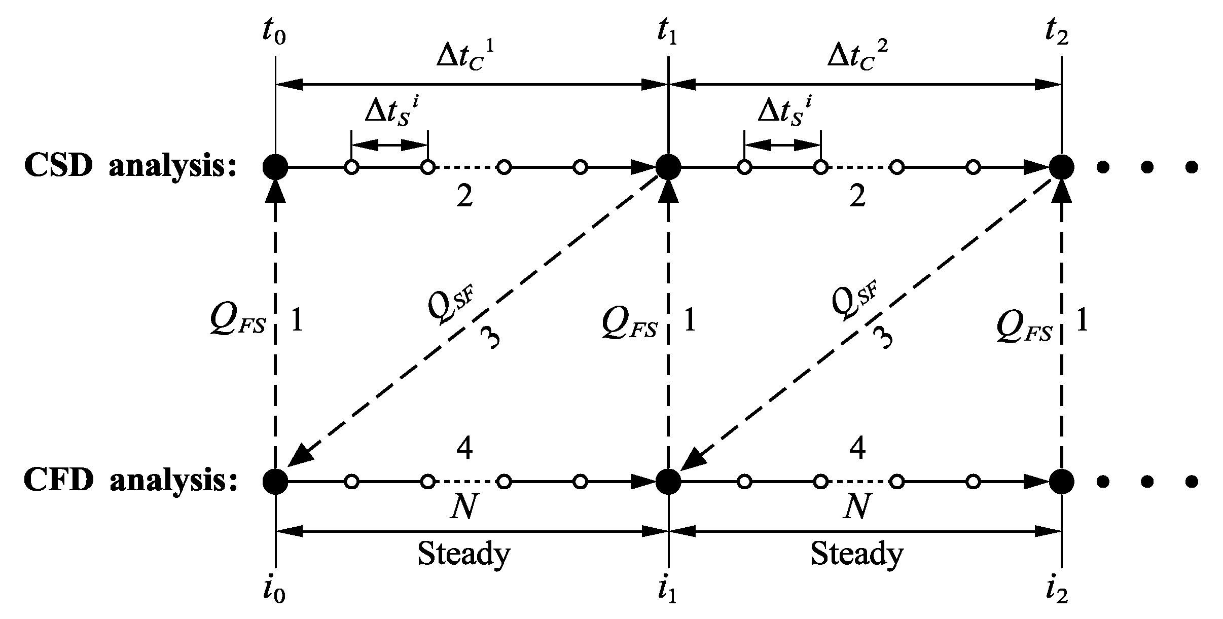
Figure 2.
Fluid–structural coupling algorithm.
Figure 2.
Fluid–structural coupling algorithm.
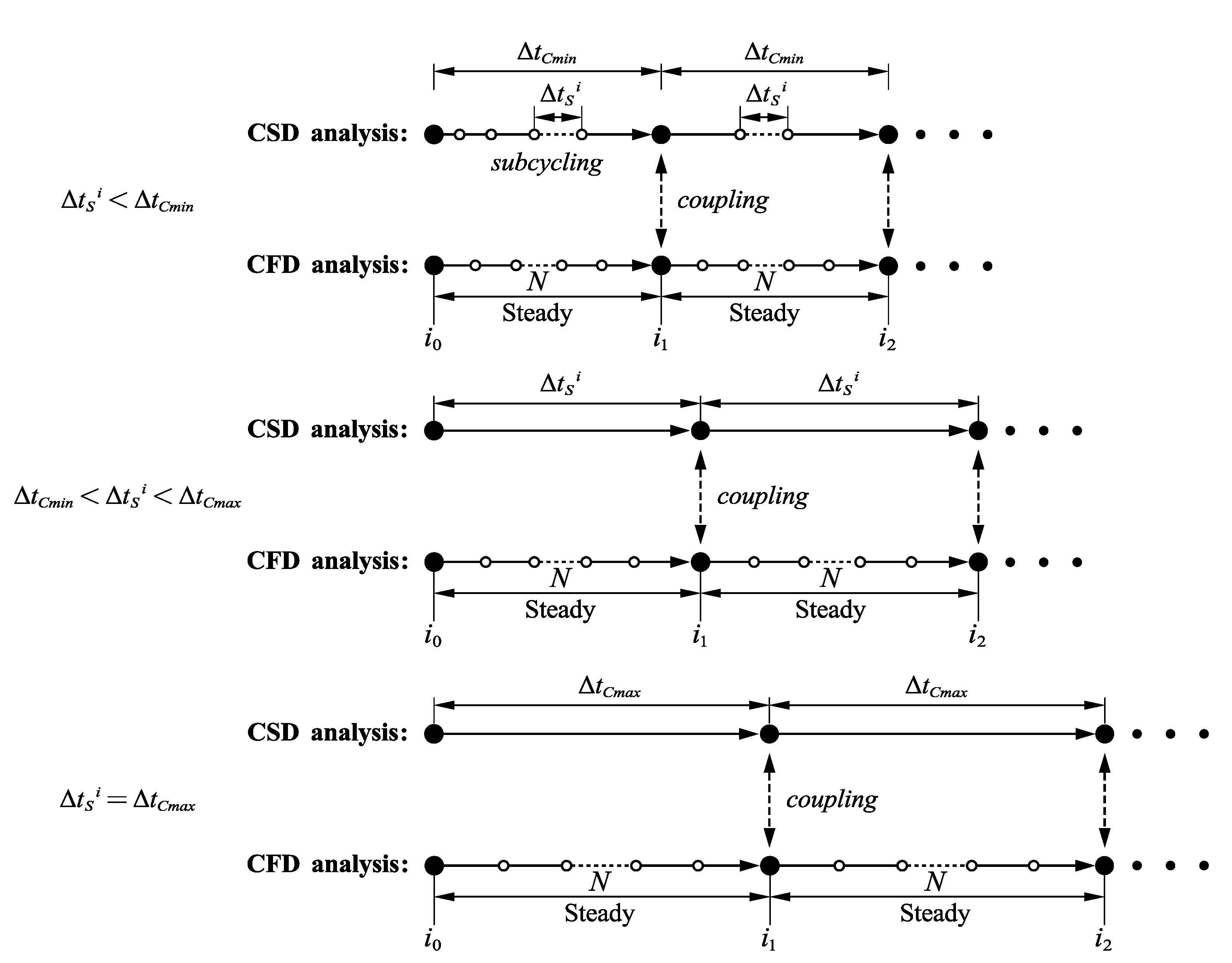
Figure 3.
The variation rules of adaptive coupling time step.
Figure 3.
The variation rules of adaptive coupling time step.
Figure 4.
Coupling of the non-matching meshes.
Figure 4.
Coupling of the non-matching meshes.
Figure 5.
Computational mesh for Aerospatiale A airfoil with extra fine mesh size.
Figure 5.
Computational mesh for Aerospatiale A airfoil with extra fine mesh size.
Figure 6.
Pressure and skin friction coefficient distribution for meshes with different densities. (a) Pressure coefficient. (b) Skin friction coefficient.
Figure 6.
Pressure and skin friction coefficient distribution for meshes with different densities. (a) Pressure coefficient. (b) Skin friction coefficient.
Figure 7.
Pressure and skin friction coefficient distribution. (a) Pressure coefficient. (b) Skin friction coefficient.
Figure 7.
Pressure and skin friction coefficient distribution. (a) Pressure coefficient. (b) Skin friction coefficient.
Figure 8.
Skin friction coefficient contour.
Figure 8.
Skin friction coefficient contour.
Figure 9.
Geometric shape of the flexible membrane airfoil.
Figure 9.
Geometric shape of the flexible membrane airfoil.
Figure 10.
Time evolution of the structural deformation of the membrane airfoil and depict of flow field streamlines.
Figure 10.
Time evolution of the structural deformation of the membrane airfoil and depict of flow field streamlines.
Figure 11.
The time-averaged deformation of the membrane airfoil at .
Figure 11.
The time-averaged deformation of the membrane airfoil at .
Figure 12.
Variation of displacement with time at the monitoring point 8.
Figure 12.
Variation of displacement with time at the monitoring point 8.
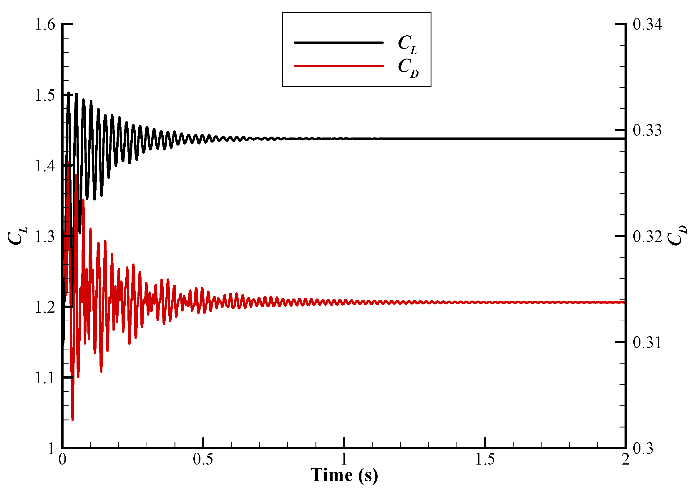
Figure 13.
Variation of lift and drag coefficient with time.
Figure 13.
Variation of lift and drag coefficient with time.
Figure 14.
Depict of the solar-powered UAV configuration.
Figure 14.
Depict of the solar-powered UAV configuration.
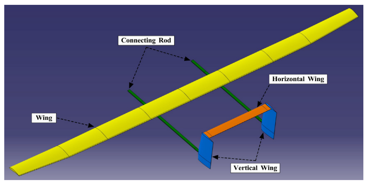
Figure 15.
Details of the solar-powered UAV configuration.
Figure 15.
Details of the solar-powered UAV configuration.
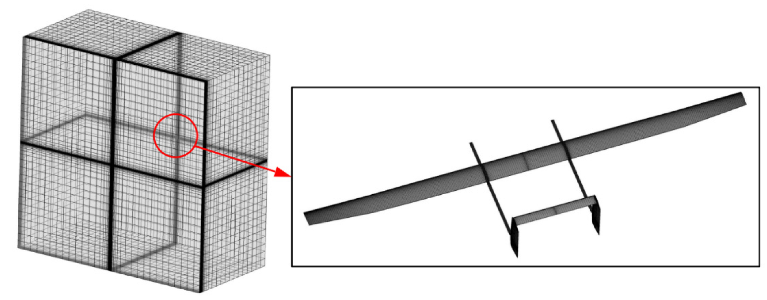
Figure 16.
Far field and surface mesh of the solar plane.
Figure 16.
Far field and surface mesh of the solar plane.
Figure 17.
Finite element model of the high-aspect-ratio wing.
Figure 17.
Finite element model of the high-aspect-ratio wing.
Figure 18.
Averaged mass distribution along the wing span.
Figure 18.
Averaged mass distribution along the wing span.
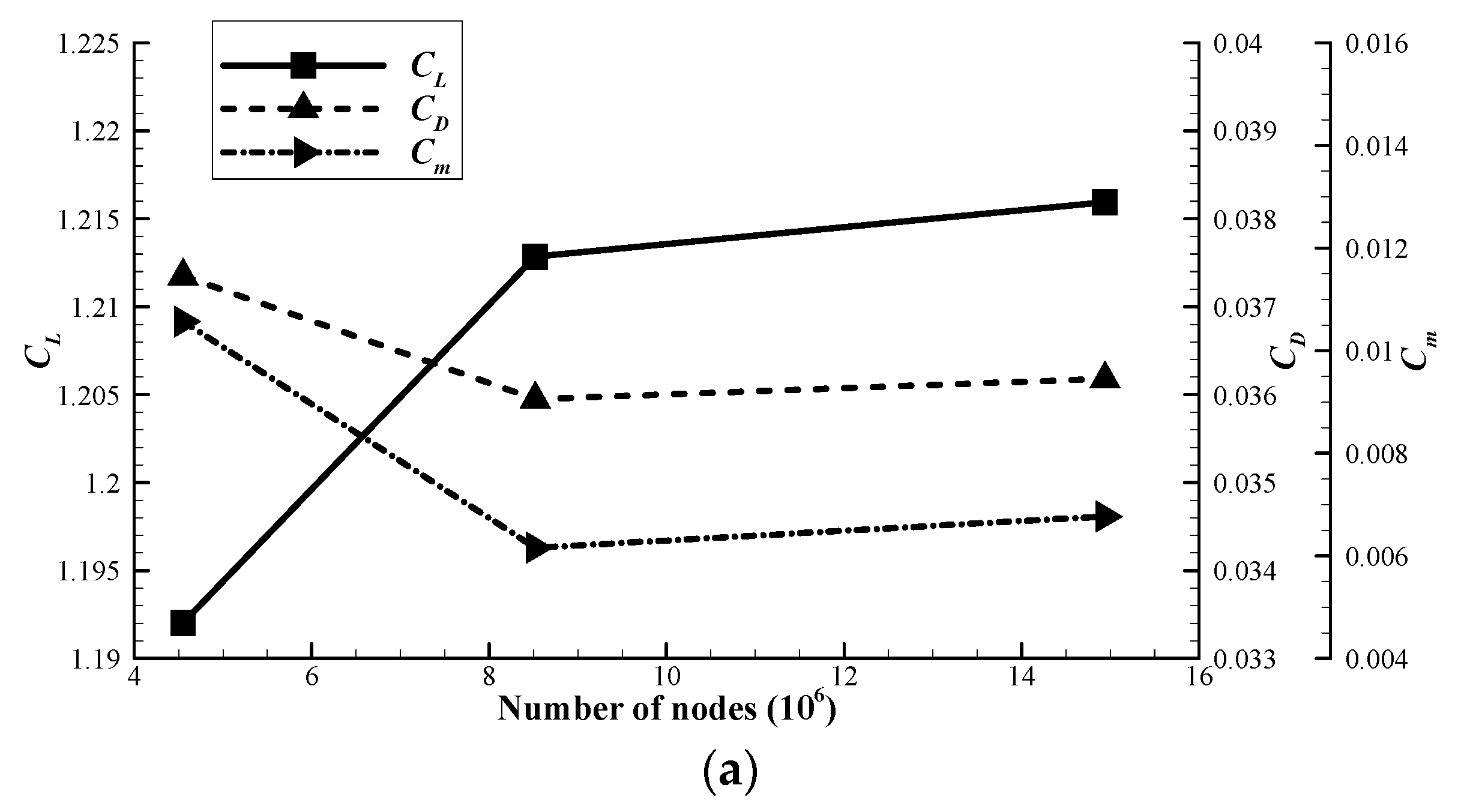
Figure 19.
Variation of the aerodynamic coefficients with mesh density. (a) . (b) .
Figure 19.
Variation of the aerodynamic coefficients with mesh density. (a) . (b) .
Figure 20.
Aerodynamic characteristics of the solar plane.
Figure 20.
Aerodynamic characteristics of the solar plane.
Figure 21.
Pressure and skin friction coefficient contour of the solar plane. (a) Pressure coefficient. (b) Skin friction coefficient.
Figure 21.
Pressure and skin friction coefficient contour of the solar plane. (a) Pressure coefficient. (b) Skin friction coefficient.
Figure 22.
The variation of adaptive coupling time step for Case B and Case C. (a) Case B. (b) Case C.
Figure 22.
The variation of adaptive coupling time step for Case B and Case C. (a) Case B. (b) Case C.
Figure 23.
Displacement distribution of beam2 along the span at in Case C.
Figure 23.
Displacement distribution of beam2 along the span at in Case C.
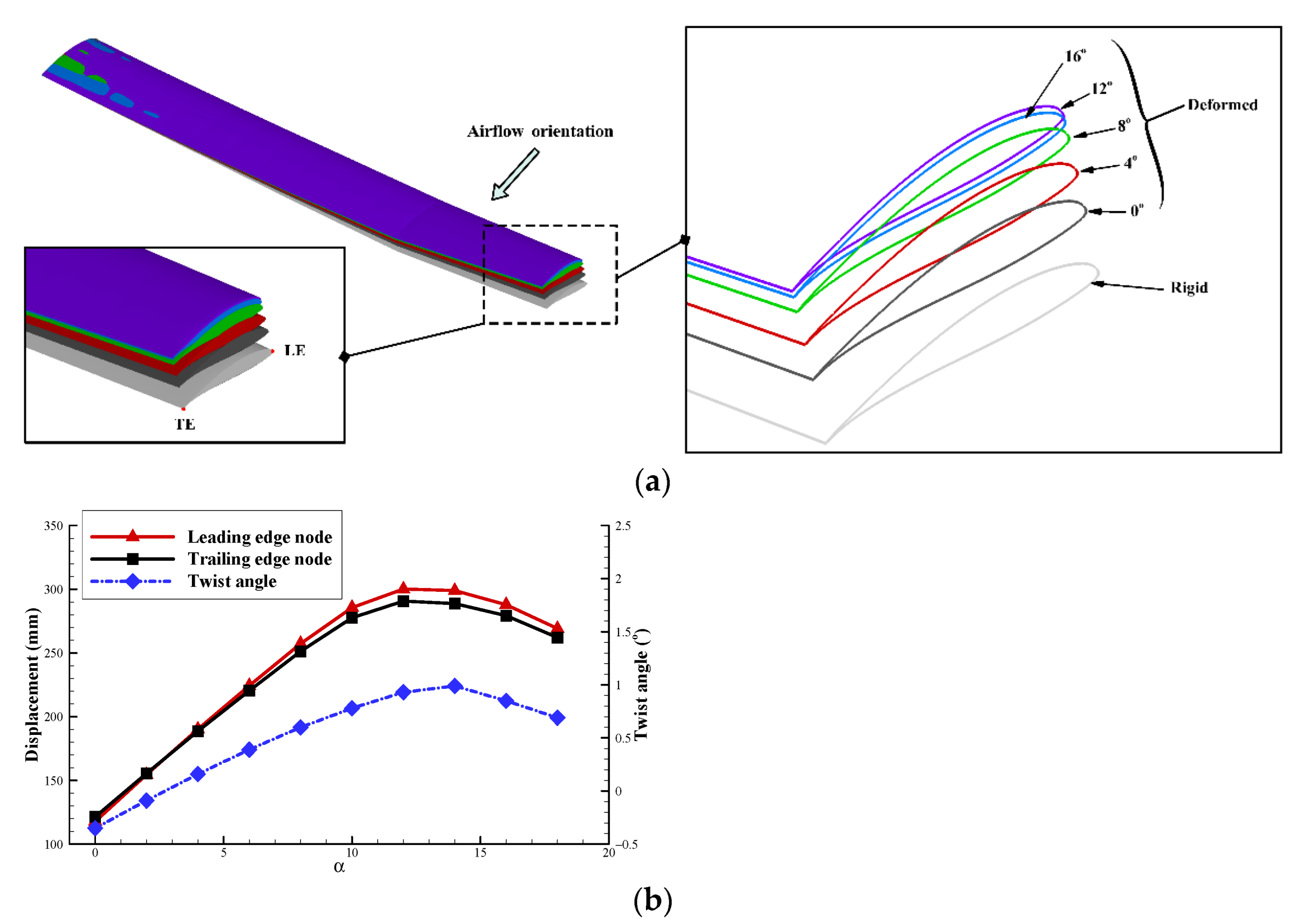
Figure 24.
Deformation of the wing. (a) Deformation of the wing at various angles. (b) Displacements and torsion angle of the wing tip.
Figure 24.
Deformation of the wing. (a) Deformation of the wing at various angles. (b) Displacements and torsion angle of the wing tip.
Figure 25.
Comparison of the profiles of the deformed wing at various incidence angles (x/z = 0.3). (a) y/b = 15%. (b) y/b = 45%. (c) y/b = 75%. (d) y/b = 95%.
Figure 25.
Comparison of the profiles of the deformed wing at various incidence angles (x/z = 0.3). (a) y/b = 15%. (b) y/b = 45%. (c) y/b = 75%. (d) y/b = 95%.
Figure 26.
Displacements of the monitor points on the flexible surface.
Figure 26.
Displacements of the monitor points on the flexible surface.
Figure 27.
Aerodynamic characteristics of the rigid and deformed wing. (a) . (b) .
Figure 27.
Aerodynamic characteristics of the rigid and deformed wing. (a) . (b) .
Figure 28.
Comparison of pressure coefficient distribution of the rigid and deformed wing at various incidence angles. (a) . (b) . (c) .
Figure 28.
Comparison of pressure coefficient distribution of the rigid and deformed wing at various incidence angles. (a) . (b) . (c) .
Figure 29.
Comparison of the transition location of the rigid and deformed wing at various incidence angles.
Figure 29.
Comparison of the transition location of the rigid and deformed wing at various incidence angles.
Figure 30.
Contour of turbulent kinetic energy on the rigid and deformed wing. (a) . (b) .
Figure 30.
Contour of turbulent kinetic energy on the rigid and deformed wing. (a) . (b) .
Figure 31.
Comparison of flow field streamlines around the rigid and deformed wing at sections along the span. (a) Wing sections along the span. (b) . (c) .
Figure 31.
Comparison of flow field streamlines around the rigid and deformed wing at sections along the span. (a) Wing sections along the span. (b) . (c) .
Table 1.
Details of the meshes.
Table 1.
Details of the meshes.
| Mesh Level | Extra Coarse | Coarse | Medium | Fine | Extra Fine |
|---|
| Number of circumferential grid points | 80 | 160 | 240 | 320 | 400 |
| Number of elements (×104) | 10 | 13 | 16 | 19 | 22 |
Table 2.
Comparison of calculation results with experimental data.
Table 2.
Comparison of calculation results with experimental data.
| Aerodynamic Coefficient | Experimental Data | Full Turbulence | Free Transition |
|---|
| Value | | Value | |
|---|
| Lift | 1.562 | 1.447 | −7.4% | 1.570 | 0.5% |
| Drag | 0.0208 | 0.0315 | 51.4% | 0.0222 | 6.7% |
Table 3.
Main geometric parameters of the solar plane.
Table 3.
Main geometric parameters of the solar plane.
| Component | Parameter | Value |
|---|
| Wing | Reference area | 12.338 m2 |
| Mean aerodynamic chord | 0.73 m |
| Span | 16.64 m |
| Aspect ratio | 22.8 |
| Span (Section A) | 5.92 m |
| Span (Section B) | 2.4 m |
| Mounting angle | 0° |
| Dihedral angle (Section A) | 0° |
| Dihedral angle (Section B) | 3° |
| Horizontal wing | Chord | 0.38 m |
| Span | 3.11 m |
| Mounting angle | −3° |
| Vertical wing | Chord | 0.638 m |
| Span | 1.11 m |
Table 4.
Details of the meshes in different level.
Table 4.
Details of the meshes in different level.
| Mesh Level | L1 | L2 | L3 |
|---|
| Number of elements (×106) | 465 | 867 | 1519 |
| Number of nodes (×106) | 455 | 852 | 1494 |
| yplus | 2 | 1 | 0.5 |
Table 5.
Material properties of the wing.
Table 5.
Material properties of the wing.
| Material | Elastic Modulus/MPa | Poisson’s Ratio | Density/(kg/m3) |
|---|
| T700 | 350,000 | 0.3 | 1590 |
| CCM40J | 210,000 | 0.3 | 1590 |
| RS50 | 114 | 0.36 | 51.3 |
| Membrane | 1000 | 0.29 | 1350 |
Table 6.
Parameters and materials of the shell components in the wing.
Table 6.
Parameters and materials of the shell components in the wing.
| Thin shell | Thickness | Material |
|---|
| Upper surface | 0.06 mm | Membrane |
| Lower surface | 0.4 mm | T700 |
| Wing front | 0.4 mm |
| Wing trailing edge | 0.4 mm |
| Ribs | 4 mm | CCM40J, RS50 |
Table 7.
Parameters and materials of the beam components in the wing.
Table 7.
Parameters and materials of the beam components in the wing.
| Beam | Section Profile (a, b) | Number of Carbon Fibre Layers (0.1 mm/Layer) | Material |
|---|
| ) | (3, 5) mm | 20 | T700, RS50 |
| ) | (2, 5) mm | 10 |
| ) | (6, 8) mm | 50 |
| ) | (2, 5) mm | 10 |
| ) | (3, 5) mm | 20 |
| ) | (2, 5) mm | 10 |
Table 8.
Details of the different computational cases.
Table 8.
Details of the different computational cases.
| Case | Case A | Case B | Case C |
|---|
| Method | Constant | Adaptive | Adaptive |
| Initial time step of CSD computation (s) | 0.001 | 0.001 | 0.001 |
| 0.05 | 0.05 | 0.05 |
| 0.05 | 0.2 | 0.5 |
| Number of coupling steps | 50 | 25 | 16 |
| (mm) | 190.29 | 190.31 | 190.35 |
| CPU time (min) | 400 | 186 | 112 |


