Strategies for Scaleable Communication and Coordination in Multi-Agent (UAV) Systems

Abstract

A system is considered in which agents (UAVs) must cooperatively discover interest-points (i.e., burning trees, geographical features) evolving over a grid. The objective is to locate as many interest-points as possible in the shortest possible time frame. There are two main problems: a control problem, where agents must collectively determine the optimal action, and a communication problem, where agents must share their local states and infer a common global state. Both problems become intractable when the number of agents is large. This survey/concept paper curates a broad selection of work in the literature pointing to a possible solution; a unified control/communication architecture within the framework of reinforcement learning. Two components of this architecture are locally interactive structure in the state-space, and hierarchical multi-level clustering for system-wide communication. The former mitigates the complexity of the control problem and the latter adapts to fundamental throughput constraints in wireless networks. The challenges of applying reinforcement learning to multi-agent systems are discussed. The role of clustering is explored in multi-agent communication. Research directions are suggested to unify these components.

1. Introduction

Advances in mobile computing, wireless technology, and artificial intelligence have fundamentally impacted the field of robotics. Applications that require persistent operation of large numbers of robots in remote areas (without pre-existing wireless infrastructure) are of special interest. 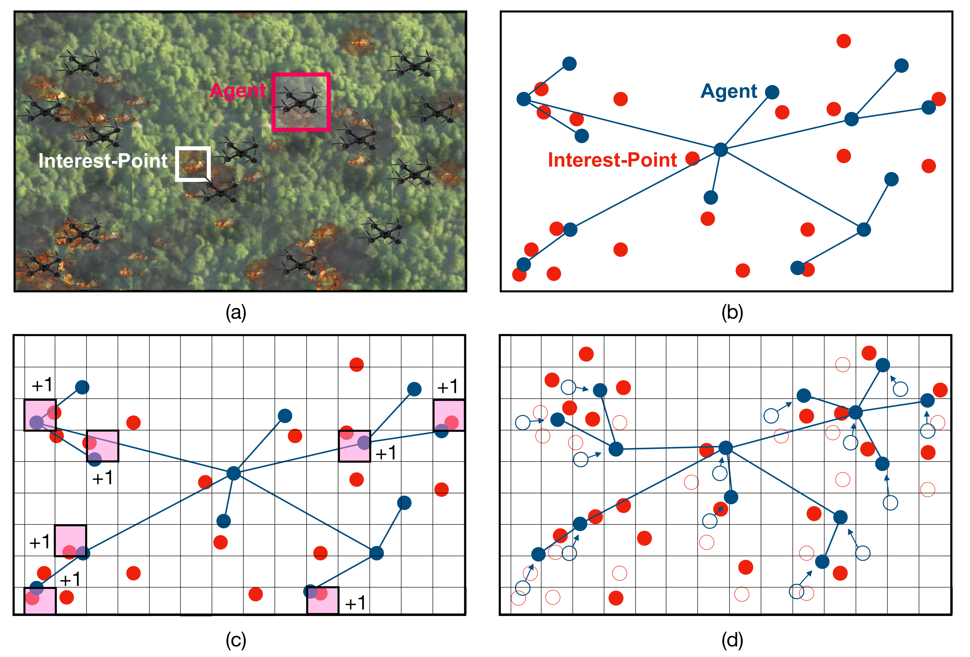Examples include wildfire surveillance [1], aerial package delivery [2], environmental surveillance [3], emergency drone-based wireless-provisioning [4], post-event perishable data-acquisition [5], and planetary exploration [6]. A common theme in these examples is the idea of spatially distributed “interest-points” (i.e., burning trees, geological features, delivery destinations) that evolve over time. The robots must collectively visit as many interest-points as possible over some bounded time-horizon as depicted in Figure 1. Despite the promise of this technology, certain control and communication problems continue to hinder large-scale deployment. Two problems are presently intractable: the communication problem, in which robots share their local states and observations, and the control problem in which robots decide on a collective action to achieve the system objectives.

An “agent” is a self-contained computational unit acting in some external environment (i.e., a robot, Unmanned Aerial Vehicle (UAV) or Autonomous Underwater Vehicle (AUV)). In distributed systems, individual agents do not have direct access to the states of other agents. Direct communication between all agent pairs is often impossible in a shared wireless medium, due to channel fading and interference. Instead, agents must discover their “neighbors” (i.e., agents in the geographic vicinity), their neighbors’ neighbors, and so on until they obtain a common view of the topology induced by this network. The agents communicate by routing messages in multi-hop fashion from one agent to the next. Their relative positions change as they move, which alters the underlying network topology and the implied communication routes. They must constantly update their views of the network topology and refresh their forwarding tables, all while sharing the local states required for coordination.

Only after the local states have been shared, are agents able to infer the global state and coordinate their actions. However, even with universal knowledge of the global state, the optimal control policy is still ambiguous. Agents could behave selfishly (or “greedily”) to maximize their “take” of interest-points, or cooperatively, favoring the benefit to the collective over the individual. They could act strategically, to obtain future returns at the expense of the present. The dynamics of the interest-points, initially unknown, also factor into these decisions. Ultimately, the decision space grows exponentially in size (or worse) with the number of agents, which makes the optimal solution unscaleable.

The control and communication problems are often separate areas of research, but there have been efforts to integrate them in the field of robotics. This survey/concept paper highlights important contributions in both areas through the lens of multi-agent tracking. Some original ideas are also presented to offer perspective on a joint control/communication architecture.

The paper is organized as follows. Section 2 reviews the basics of reinforcement learning (RL) with an eye towards multi-agent tracking systems. Section 3 explores the control problem; the complexity of computing control policies in multi-agent RL and the challenge of verifying whether or not these policies are optimal. Methods that exploit locally interactive structure are discussed to alleviate these challenges. Section 4 explores aspects of the communication problem: the fundamental constraints on throughput in wireless networks and the unreliable nature of wireless communication. Multi-level clustering strategies are surveyed as a possible antidote. Section 5 discusses whether the selected works in this survey fit into a unified architecture that encompasses both the control and communication aspects of multi-agent systems. Section 6 concludes the paper and highlights new research directions.

2. Reinforcement Learning

The famous Travelling Salesman Problem (TSP) asks for the shortest path that touches all vertices in a graph. In the worst-case, the answer requires exponentially many operations in the number of vertices. However, computing the distance of any arbitrary path requires at most a polynomial (or linear) number of operations. This property is distinctive of “NP-hard” problems (i.e., non-deterministic polynomial); optimal solutions seemingly have exponential complexity, but candidate solutions have polynomial complexity. A long-standing open problem in complexity theory is proving (or disproving) P ≠ NP; whether or not “NP-hard” problems can be solved in polynomial-time.

Multi-agent tracking is a more complicated version of the TSP because there are multiple agents (i.e., salesmen), the graph topology is time-varying, and the agent trajectories must remain disjoint at each time-instant. The complexity of any solution is thus worse than exponential in the number of agents. While the TSP remains an important benchmark in theoretical computer science, there is also interest in approximately optimal but low-complexity solutions for engineering applications.

Reinforcement learning (RL) offers these “engineering” solutions to high-complexity path-planning problems. The challenge is stabilizing the learning process within a reliably acceptable time-frame. Apart from some narrowly defined scenarios, no such convergence guarantees exist. The following sections introduce basic concepts in RL and discuss their relevance to multi-agent tracking.

2.1. Overview

The Markov Decision Process (MDP) consists of three components: states, actions, and rewards. The system state is a snapshot of all the parameters of interest in a given time-instant. These parameters are application-specific but usually include data such as the agents’ positions, velocities, altitudes and/or any other items relevant to the system operation. Actions cause the system to change from one state to another (i.e., actions such as “right”, “left”, “up”, and “down” move individual agents in a two-dimensional grid to adjacent cells). Rewards assign value to desirable states and/or penalize undesirable states. 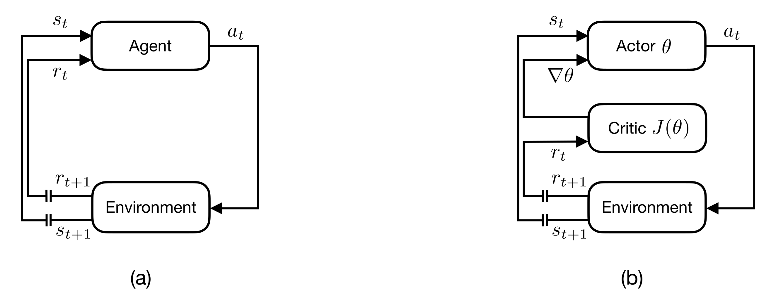For instance, states in which agents and interest-points overlap might receive positive reward as depicted in Figure 1c, whereas states in which two agents occupy the same cell (i.e., have collided) receive negative reward. This acts as a signal from environment to agent, encouraging certain behavior. The agent-environment feedback loop is depicted in Figure 2a. A policy determines the action of an agent in every state. The objective in RL is to compute the optimal policy; the policy that achieves the maximum reward over the operating lifetime.

The Markov property limits the way states can evolve over time, namely, that future states are conditionally independent of past states given the current state; the future depends only on the past through the present. Another concept related to the Markov property is “stationarity”. The system is stationary if the “dynamics” (i.e., the probabilities of transitioning from one state to another) do not change over time. Stationary dynamics are the default assumption in RL. However, strategies that reduce complexity (i.e., shorten training times) sometimes induce time-varying dynamics as an unintended side-effect.

2.2. The System State Space

In multi-agent systems, the notion of a “state” has a local and a global meaning. Local states refer to individual agents, whereas global or system states include all the individual local states and other relevant parameters (such as the positions of the interest-points in tracking applications).

A key challenge in multi-agent RL is the exponential growth of the state-space in the number of agents. A single agent system on a 10 × 10 grid has at minimum 100 possible states (if each state corresponds to a coordinate position). However, an n-agent system on the same 10 × 10 grid has ${100}^n$ possible states.

Locally interactive structure will often be referenced in this paper to reduce computational complexity (Section 3) and satisfy fundamental communication constraints (Section 4). This property implies that activity occurring in remote areas of the grid relative to any agent, is less relevant to the optimal behavior of that agent than activity nearby [7,8]. Each agent can then simplify the global state it “sees” while staying responsive to global/system-level objectives.

Another challenge in multi-agent systems is that agents only observe their local states (not the global state). “Partially-Observable” MDPs (or POMDPs) allow observations to stochastically depend on the underlying global state. POMDPs are more complicated than MDPs and fall outside the scope of this survey. However, other ways of extending the MDP framework to multi-agent systems are discussed in Section 3.

2.3. Rewards

The reward function assigns a real-valued number to each state. Higher rewards incentivize desirable states (i.e., states in which interest-points and agents overlap) whereas negative rewards discourage undesirable states (i.e., states in which positions of two agents coincide), as depicted in Figure 1c. The objective in RL is to determine behavior that maximizes the expected reward over the operating lifetime.

2.4. Actions, Policies, and Value Functions

A policy $\pi \left(s\right)$ defines the actions $a_i\in {\mathcal{A}}_i$ of each agent $i\in \mathcal{N}$ in the current state $s\in \mathcal{S}$ where $\mathcal{N}$ is the set of all agents, ${\mathcal{A}}_i$ is the set of all possible actions at agent i and $\mathcal{S}$ is the set of all possible states (in the multi-agent system). That is, for some joint action $\mathbf{a}=(a_1,a_2,\dots ,a_{\left|\mathcal{N}\right|})$:

$$\begin{array}{c}\hfill \pi \left(s\right):=\mathbf{a}.\end{array}$$

(1)

Local policies ${\pi }_i\left(s\right)$ define the actions $a_i$ of a particular agent $i\in \mathcal{N}$, whereas global policies $\pi \left(s\right)=({\pi }_1\left(s\right),{\pi }_2\left(s\right),\dots ,{\pi }_{\left|\mathcal{N}\right|}\left(s\right))$ define the actions of all $\left|\mathcal{N}\right|$ agents simultaneously (i.e., all the individual local policies). The actions executed by all agents collectively form the “joint” action $\mathbf{a}$. In distributed systems, each agent only has direct access to its local state, so any joint-action requires some form of system-wide inter-agent communication to infer $s\in \mathcal{S}$.

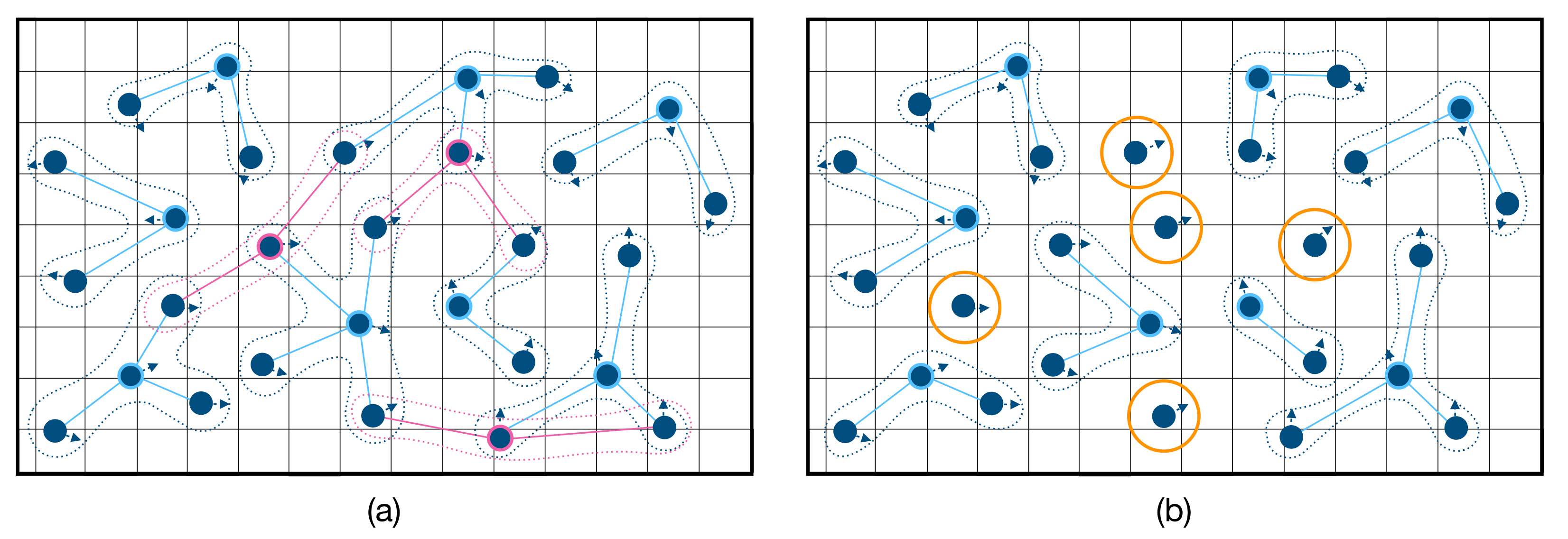
In applications where the system has locally interactive structure, agents can prioritize the local states of other agents in their vicinity over agents further away, to reduce the total information throughput [9,10]. Each agent then obtains a unique view of the state space, with decreasing resolution in regions of the grid more remote from its current position. Even though each agent has different views, the joint-action is still approximately optimal provided the remote areas have enough resolution to capture “lower-order” trends. This trade-off between information throughput and overall tracking performance is further explored in Section 3 and Section 4.

Every policy $\pi \left(s\right)$ at state $s\in \mathcal{S}$ has an associated value $V_{\pi }\left(s\right)$, defined as the expected discounted reward received over the operating lifetime. $V_{\pi }\left(s\right)$ is called the value function for the policy $\pi$. Let $S_t$, $A_t$, and $R_t$ be random variables that denote the system state, action, and reward respectively at time t. Let $\gamma$ denote the discount factor which, like an interest rate, discounts the rewards expected in the future over rewards in the present. Then $V_{\pi }\left(s\right)$ is defined as:

$$\begin{array}{c}\hfill V_{\pi }\left(s\right):=E_{\pi }\left[\sum _{k=0}^{\infty }{\gamma }^k{R}_{t+k}|S_t=s\right].\end{array}$$

(2)

Let ${\pi }^{*}\left(s\right)$ denote the policy with the highest value $V^{*}\left(s\right)$ (i.e., the optimal policy):

$$\begin{array}{cc}\hfill V^{*}\left(s\right)& :=\underset{\pi }{max}{V}_{\pi }\left(s\right),\hfill \end{array}$$

(3)

$$\begin{array}{cc}\hfill {\pi }^{*}\left(s\right)& :=arg\underset{\pi }{max}{V}_{\pi }\left(s\right).\hfill \end{array}$$

(4)

The main objective in RL is to compute the ${\pi }^{*}\left(s\right)$ defined in (4). The optimizations in (3) and (4) satisfy the following fundamental property:

$$\begin{array}{cc}\hfill V^{*}\left(s\right)& :=\underset{\mathbf{a}}{max}{E}_{\pi }\left[R_t+\gamma V^{*}\left(S_{t+1}\right)|S_t=s,A_t=\mathbf{a}\right]\hfill \end{array}$$

(5)

Equation (5) follows from Bellman’s Principle of optimality which says that any segment in the shortest path between two points is the shortest sub-path between the segment endpoints. In this case, the “shortest” path is the trajectory of states that achieves the maximum discounted reward in (2).

For most applications, it is not practical to compute (3) and (4) directly since there are exponentially many trajectories in the size of the state space $\left|\mathcal{S}\right|$. The fixed-point equation in (5) reduces this complexity, but not to the extent that direct computations are feasible.

Deep RL finds approximate solutions to (3). The value function $V_{\pi }\left(s\right)$ is modeled by a neural network. Instead of directly computing (3), RL samples from the next reachable subset of states and observes the accrued reward. If the neural network is sufficiently deep and the subset of sampled states is sufficiently large, there is a decent chance the estimate ${\widehat{V}}_{\pi }\left(s\right)$ will converge to the actual $V_{\pi }\left(s\right)$. There is no formal proof of this statement, only compelling experimental results and simulations [11,12].

The fixed-point Equation (5) still plays a key role in deep RL, albeit indirectly through the “update rule”. Each new observation feeds into a running estimate ${\widehat{V}}_{\pi }\left(s\right)$ of $V_{\pi }\left(s\right)$:

$$\begin{array}{c}\hfill {\widehat{V}}_{\pi }\left(S_t\right)+\alpha (R_{t+1}+\gamma {\widehat{V}}_{\pi }\left(S_{t+1}\right)-{\widehat{V}}_{\pi }\left(S_t\right))\to {\widehat{V}}_{\pi }\left(S_t\right).\end{array}$$

(6)

The parameter $\alpha$ refers to the sensitivity of the estimate to the newly acquired data (the observed reward $R_{t+1}$). The update rule in (6) is called the “Bellman update”. In deep RL, the difference between the update and the previous estimate (the loss function) drives the parameters of the neural net in the direction of the update via stochastic gradient descent.

2.5. Value Iteration vs Policy Iteration

An important measure of value called the “Q” function $Q_{\pi }(s,\mathbf{a})$ also depends on the next action $\mathbf{a}=\pi \left(s\right)$:

$$\begin{array}{c}\hfill Q_{\pi }(s,\mathbf{a})=E_{\pi }\left[\sum _{k=0}^{\infty }{R}_{t+k}|S_t=s,A_t=\mathbf{a}\right].\end{array}$$

(7)

Let $Q^{*}(s,\mathbf{a})$ denote optimal Q-value at state s from following the optimal action $\mathbf{a}={\pi }^{*}\left(s\right)$:

$$\begin{array}{cc}\hfill Q^{*}(s,\mathbf{a})& :=\underset{\pi }{max}{Q}_{\pi }(s,\mathbf{a}),\hfill \end{array}$$

(8)

$$\begin{array}{cc}\hfill {\pi }^{*}\left(s\right)& :=arg\underset{\pi }{max}{Q}_{\pi }(s,\mathbf{a}).\hfill \end{array}$$

(9)

The Q-function also satisfies a fixed-point equation:

$$\begin{array}{c}\hfill Q^{*}(s,\mathbf{a})=\underset{\mathbf{a}}{max}{E}_{\pi }[R_t+\gamma Q^{*}(S_{t+1},A_{t+1})|S_t=s,A_t=\mathbf{a}].\end{array}$$

(10)

Both notions of value $Q_{\pi }(s,\mathbf{a})$ and $V_{\pi }\left(s\right)$ support two fundamentally different approaches in RL: value iteration and policy iteration. The actor-critic approach, associated with policy iteration maintains two parallel estimates: the “actor” is one in a family of policies $\{{\pi }_{\theta }:\theta \in \Theta \}$ parameterized by $\theta$ whereas the critic is an estimate of the value of the current policy $J(\theta ):=E_{{\pi }_{\theta }}\left[V_{{\pi }_{\theta }}\left(s\right)\right]$, as depicted in Figure 2. Each sequence of updates cycles between the actor and critic, waiting for $J(\theta )$ to stabilize before altering the current policy ${\pi }_{\theta }$ to one better [13,14].

Q-learning by contrast, associated with value iteration, only maintains an estimate of the Q-function $Q_{\pi }(s,\mathbf{a})$ [15]. The policy ${\pi }_g$ that explores the state-space is the “greedy” policy:

$$\begin{array}{cc}\hfill {\pi }_g\left(s\right)& :=arg\underset{\mathbf{a}}{max}{Q}_{\pi }(s,\mathbf{a}).\hfill \end{array}$$

(11)

The unusual feature of (11) is that the greedy policy ${\pi }_g$ is different from the $\pi$ of $Q_{\pi }(s,\mathbf{a})$ (which generates ${\pi }_g$); Q-learning does not wait for the estimate $Q_{\pi }(s,\mathbf{a})$ to stabilize before altering the policy to ${\pi }_g$. Nevertheless, there is mathematical proof that ${\pi }_g$ converges to ${\pi }^{*}$ if it is sufficiently “exploratory” (i.e., samples a large enough subset of the state-space infinitely often); the “max” operation in (11) is an infinity-norm with a telescoping property in the policy space [16]. The literature often asserts that Q-learning has shorter convergence times due to this aggressive update strategy.

2.6. The Deadly Triad

Two fundamental components of deep RL are the neural net approximation of $V_{\pi }\left(s\right)$ (denoted by the estimate ${\widehat{V}}_{\pi }\left(s\right)$) together with Bellman updates of the estimate based on (6). Each update of ${\widehat{V}}_{\pi }\left(s\right)$ is formed (or ”bootstrapped”) from previous values of ${\widehat{V}}_{\pi }\left(s\right)$. These strategies are called “function-approximation” and “bootstrapping” in the literature. A special name belongs to the type of strategy in Q-Learning, where the policy being followed (to explore the state-space) differs from the policy being evaluated. This strategy is called “off-policy learning”.

The “deadly triad” is a problem that emerges when function approximation, bootstrapping, and off-policy learning are combined [17]. Under certain conditions the learning process is guaranteed to diverge from the true optimal policy. This implies that universal convergence guarantees to the optimal policy are impossible.

One partial antidote to the deadly triad is a technique called “experience-replay”. The idea is to store state-action-reward experiences in a replay buffer. The Bellman update randomly samples from experiences in this buffer to avoid any correlation between successive samples. Stochastic gradient descent, which trains the neural network approximation of $V_{\pi }\left(s\right)$, requires independent samples to move in the direction of the local minimum. Many improvements and enhancements of experience-replay have since been proposed [18,19]. The deadly triad remains an active area of research.

3. Multi-Agent Planning and Control

Multi-agent systems present two distinct challenges. First, there is a “control” problem caused by the exponential growth of the state space in the number of agents. Second, there is a communication problem of sharing all the local states so that the agents arrive at a common view of the global state. The communication problem is addressed in Section 4, so the default assumption here will be that each agent sees the global state space.

Large state spaces require longer training times because the training process must sample a sufficiently large subset of the state space $\mathcal{S}$, sufficiently often, to learn both $V_{\pi }\left(s\right)$ and the optimal policy ${\pi }^{*}\left(s\right)$ for all $s\in \mathcal{S}$. An important strategy to shorten the training times is state-space compression. The idea is to map the old state space $\mathcal{S}$ to a new space $f:\mathcal{S}\to {\mathcal{S}}^{\prime }$ where

$$\begin{array}{c}\hfill |{\mathcal{S}}^{\prime }|<<|\mathcal{S}|\end{array}$$

(12)

but ${\pi }^{*}\left(s\right)\approx {\pi }^{*}\left(f\left(s\right)\right)$, or equivalently:

$$\begin{array}{c}\hfill V_{\pi }^{*}\left(s\right)\approx V_{\pi }^{*}\left(f\left(s\right)\right).\end{array}$$

(13)

The value on the left side of (13) is obtained from the optimal policy ${\pi }^{*}\left(s\right)$ over $\mathcal{S}$ and the value on the right is optimal over ${\mathcal{S}}^{\prime }$. The constraint (13) implies that ${\mathcal{S}}^{\prime }$ retains all of the important information in $\mathcal{S}$, namely, the information that allows the system of robots to behave optimally with respect to $\mathcal{S}$. The compression rate in (12) usually implies polynomial (as opposed to exponential) growth in the number of agents n, so that:

$$\begin{array}{c}\hfill |{\mathcal{S}}^{\prime }|=O\left(p\left(n\right)\right)\mathrm{as}n\to \infty ,\end{array}$$

(14)

where $p\left(n\right)$ is some polynomial function of n.

If a compression f satisfying (13) exists, then it suffices to sample ${\mathcal{S}}^{\prime }$ instead of $\mathcal{S}$ (which has fewer states and thus shorter convergence times). A key objective is finding such an f and understanding the conditions for its existence.

Although the communication problem does not appear in (13) and (14), the fact remains that individual agents do not see the global state $\mathcal{S}$. Let $\mathcal{N}$ denote the set of agents. Each agent $i\in \mathcal{N}$ makes a unique reconstruction of the global state ${\mathcal{S}}_i^{\prime }$ from the local states shared through the communication medium. Ideally, these reconstructions are identical so that ${\mathcal{S}}_i^{\prime }={\mathcal{S}}^{\prime }$ for all $i\in \mathcal{N}$. However in light of the communication problem, it is better to relax this constraint and allow different reconstructions. Each agent i then effectively applies a unique compression $f_i:\mathcal{S}\to {\mathcal{S}}_i^{\prime }$. The local policies ${\pi }_i\left(f_i\left(s\right)\right)$ act on ${\mathcal{S}}_i^{\prime }$ and collectively define the global policy $\pi \left(s\right)=({\pi }_1\left(f_1\left(s\right)\right),{\pi }_2\left(f_2\left(s\right)\right),\dots ,{\pi }_{\left|\mathcal{N}\right|}\left(f_{\left|\mathcal{N}\right|}\left(s\right)\right)$. The objective then is to find the full suite of compression functions $\{f_i:i\in \mathcal{N}\}$ that achieves (13).

The distributed compression approach (above) simplifies the control problem because the global state-space $\mathcal{S}$ has locally interactive structure. Relative to any given agent, the local states in its vicinity are more significant to its optimal operation than local states that are further away. A “good” compression function $f_i$ prioritizes these local states over remote states, but also includes enough remote information to capture lower-order phenomena.

One enduring ambiguity in deep RL is the absence of any guarantees the recovered policies are optimal. Neural networks have no known bounds on the accuracy of their approximations, and the training itself relies on stochastic gradient descent, which converges only to a local optimum. This ambiguity is further exacerbated in the multi-agent setting, where distributed compression alters the states seen by each node; there is a trade-off between the compression rates corresponding to $\{f_i:i\in \mathcal{N}\}$ and the policy performance of $\pi \left(s\right)$. The next sections will explore different approaches in RL that exploit locally interactive structure in the state space.

3.1. Locally Interactive State Spaces

Every state space typically has a restricted set of legitimate transitions between individual states. This property is present in the simple gridworld system for example, with one robot on a 10 × 10 grid. Suppose the robot has four possible actions: “up”, “down”, “left”, and “right”. There are 100 possible states in the system corresponding to unique squares on the gird where the robot could be located. However, the robot can only reach (at most) four adjacent squares on the grid in the next time-step.

By definition, the state $s\in \mathcal{S}$ and the subset $X\subseteq \mathcal{S}$ are locally interactive if ${\sum }_{x\in X}p\left(x\right|s)=1$, where $\mathcal{S}$ is the set of all possible states. Locally interactive states are reachable in the next time-step, and transitions between any pair of states occur exclusively through sequences of local interactions. It is difficult to find formal methods of identifying and exploiting locally interactive structure in general state spaces, but there have been attempts in the literature to do so [20]. Examples include the “factored” MDP (F-MDP) [7,10] and POMDP (F-POMDP) [8]. Both require an explicit locally interactive structure in the state-space.

3.2. Soft Locally Interactive Structure

Multi-agent tracking exhibits a more subtle “soft” form of locally interactive structure. Suppose the interest-point locations are actually known beforehand (in practice, the agents must explore the grid and share their observations to determine these locations). The optimal policy (that visits the most interest-points) solves a more difficult version of the Travelling Salesman Problem. It requires an exhaustive search of all possible paths over the grid, enumerating the length of each path, and selecting the path of shortest length. There are exponentially many such paths in the size of the grid and number of agents. The following argument based on “soft” locally interactive structure yields an “approximately” optimal policy without the exponential complexity of an exhaustive search.

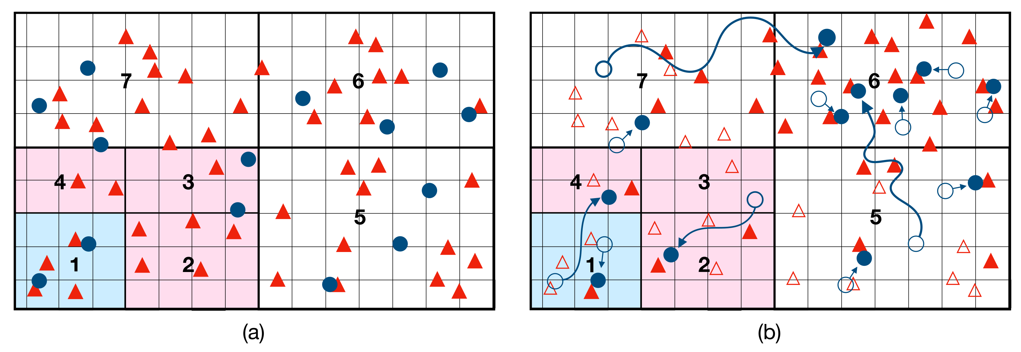
There are two scenarios to consider: one where the normalized distribution of agents matches the distribution of interest-points, and the other where the two distributions differ. In the first scenario, agents visit the interest-points in their immediate vicinity to maximize the total number of visitations. In the second, some (or all) of the agents must first re-deploy to areas of the grid that are under-served to restore the equilibrium between both distributions, so they can resume visiting interest-points in their immediate vicinity. Thus, as long as the system remains in scenario one, the tracking problem is locally interactive; the interest-points in the immediate vicinity of each agent take precedence over the interest-points further away. Only when the distributions diverge, does remote activity affect the optimal behavior of any given agent. The overall effect is a soft locally interactive structure, where the system is mostly in the equilibrium of scenario one. This situation is depicted in Figure 3.

The performance of ${\pi }^{*}\left(f\left(s\right)\right)$ in (13) depends in part on the compression loss (i.e., the loss of useful information) which occurs when the compression functions $\{f_i:i\in \mathcal{N}\}$ do not perfectly conform to the locally interactive-structure in $\mathcal{S}$. It is difficult to quantify this loss without solving the multi-robot TSP problem alluded to earlier.

3.3. Performance Metrics

A low-complexity upper-bound on the performance of ${\pi }^{*}\left(s\right)$ can be derived by computing in each time-slot, the distribution of agents that matches the distribution of interest-points. Let $P\left(t\right)=\{(x_n,y_n):n\in \mathcal{N}\}$ denote the robot positions, let $\mathcal{I}\left(t\right)$ denote the set of interest-points and let $I\left(t\right)=\{(u_i,v_i):i\in \mathcal{I}\left(t\right)\}$ denote the interest-point positions all at some fixed time-slot t. The optimal distribution $P^{*}\left(t\right)$ minimizes the distance between the agents and interest-points:

$$\begin{array}{cc}\hfill P^{*}\left(t\right)& :=arg\underset{P\left(t\right)}{min}\sum _{n\in \mathcal{N}}\sum _{i\in \mathcal{I}\left(t\right)}\left|\right|(x_n,y_n)-(u_i,v_i)\left|\right|,\hfill \end{array}$$

(15)

where $\left|\right|·\left|\right|$ is the Euclidean distance. Given robot positions $P\left(t\right)$, define the distance from agent n to its closest interest-point:

$$\begin{array}{cc}\hfill d_{P\left(t\right)}\left(n\right)& =\underset{i\in \mathcal{I}\left(t\right)}{min}\left|\right|(x_n,y_n)-(u_i,v_i)\left|\right|.\hfill \end{array}$$

(16)

Let $d^{*}$ denote the average minimum distance over all robots:

$$\begin{array}{c}\hfill d^{*}=\frac{1}{\left|\mathcal{N}\right|}\sum _{n\in \mathcal{N}}\frac{1}{T}{\int }_0^T{d}_{P^{*}\left(t\right)}\left(n\right)dt,\end{array}$$

(17)

where T is the operating lifetime. The minimum average time elapsing between two sequentially visited interest-points is $\frac{d^{*}}{v_{max}}$ where $v_{max}$ is the maximum velocity of the agent. An upper bound on the maximum number of interest-points visited by ${\pi }^{*}\left(f\left(s\right)\right)$ is given by:

$$\begin{array}{c}\hfill \frac{v_{max}T}{d^{*}}\left|\mathcal{N}\right|.\end{array}$$

(18)

Equations (15)–(18) give an approximately optimal performance metric, apart from the multi-agent TSP, that can be evaluated during simulation. They show whether or not ${\pi }^{*}\left(f\left(s\right)\right)$ satisfies (13). Alternatives to (15) for measuring the distance between distributions include the Kullback-Leibler divergence (or mutual information).

The convergence properties of multi-agent RL with state-space compression, is an ongoing area of research. One sub-topic of interest is mean-field RL, which explores the asymptotic behavior of the system as the number of agents goes to infinity. Each agent observes the sum of the local states, which is a form of distributed state-space compression. It has been shown that a Nash equilibrium in the value function exists [21].

3.4. Hierarchical Reinforcement Learning

The discussion thus far has focused on compressing the state-space, one of two factors driving complexity. The other factor is the size of the action-space, which also increases exponentially in the number of robots. If each robot has four possible actions (“up”, “down”, “left”, and “right”), then the number of possible joint actions is $4^{\left|\mathcal{N}\right|}$.

Hierarchical reinforcement learning (HRL) is a strategy for compressing action spaces [22]. The key idea in HRL is “options” (i.e., macro-actions) which specify sequences of primitive actions (“up”, “down”, “left”, and “right”) that take effect over single time-steps. Lower policies specify primitive actions, whereas higher policies specify options. The system policy is an appropriate fusion of these higher and lower policies. If the policy levels are independent, they can be trained separately. In reality, policy levels are inter-dependent and must be untangled in order for separate training to work properly.

In multi-agent tracking, higher policies issue directives such as “move from region A to region D”, as depicted in Figure 3b. Options that execute this directive rely on sequences of lower policies such as “move from region A to B”, “move from region B to C”, “move from region C to D”. Once the robot is in region D, the higher policy may issue new directives such as “find interest-points within region D”, which correspond to different option sequences.

There is a natural relationship between HRL and soft locally interactive structure in the state space; higher-order policies respond to aggregated (i.e., large-scale) phenomena of the kind that is not lost when the state-space is compressed. This relationship between action-space and state-space compression, deserves further attention in the literature.

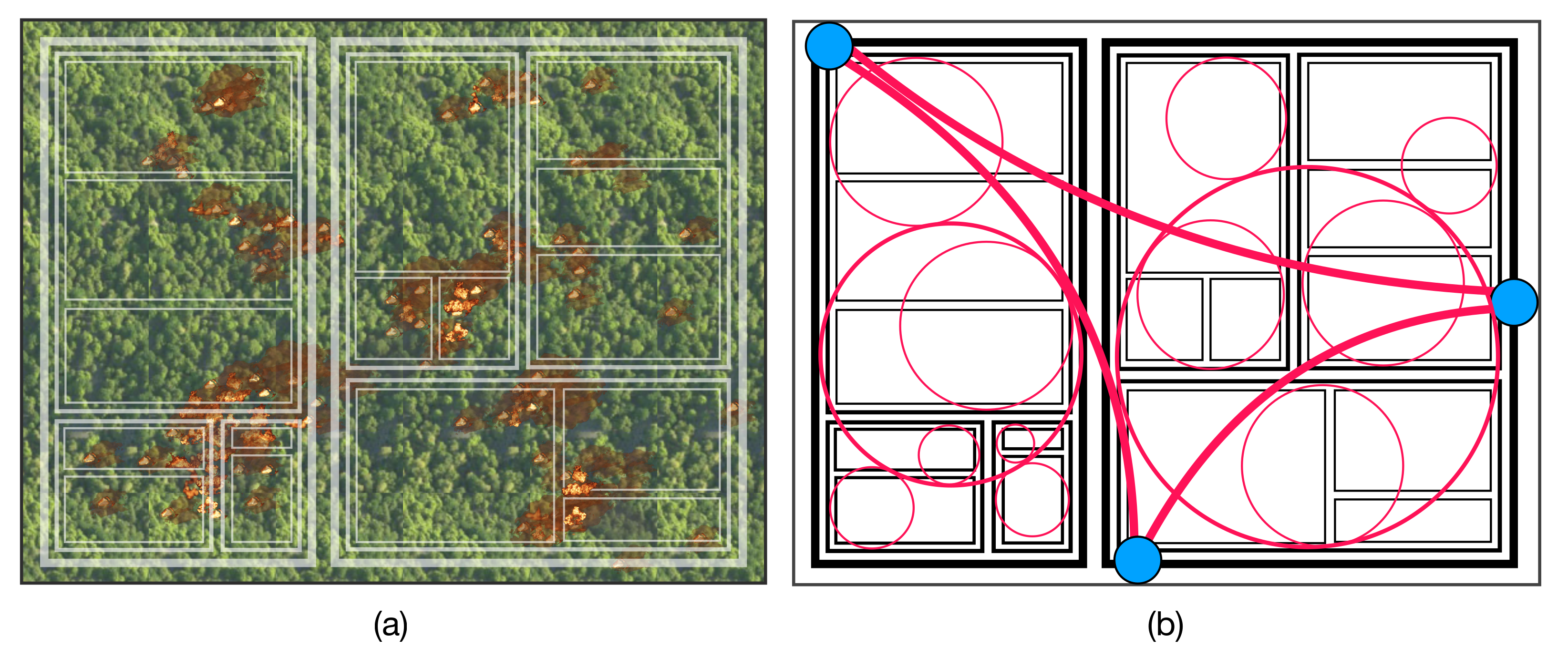
Option-spaces also grow exponentially with respect to the time-horizon window. For example, given the previous four primitive actions and a horizon of T time-steps, the number of possible options is $4^T$. Some of these options are equivalent, in that they share the same start and end-points and have similar trajectories. To compress the option-space, each equivalence class can be reduced to an exemplar from the class. The problem is then choosing equivalence classes that don’t sacrifice too much in the way of performance. This problem is largely application-specific. In multi-robot tracking, the ideal compressed option-space corresponds to a dynamic aerial transportation network, as depicted in Figure 4.

Unmanned Aerial Traffic Management (UTM) systems, which allocate airspace to UAVs on-demand, are a current topic of interest in the aerospace community. There is clear overlap in scope between option-spaces in RL and airspace assignment which has yet to be fully explored.

A major challenge in HRL is applying the ideas in Section 2 to each policy level of the option-space. Part of the problem is appropriately choosing the reward function for each sub-task, to achieve the desired net effect over all policy levels [23]. One family of strategies, based on the actor-critic approach, is the option-critic where each policy-level is assigned its own actor (estimate of the policy) and critic (value of the policy) [24]. There are numerous variations of this approach [25,26,27].

Q-Learning presents a different challenge rooted in the deadly triad of Section 2, where sampling from an experience-replay buffer makes successive updates look independent to the stochastic gradient descent algorithm. When this technique is used in HRL, older “experiences” may include lower-level options that have since changed in training; the system (viewed from any higher policy level) is no longer stationary. HIRO (Hierarchical Reinforcement Learning with Off-Policy Correction) deals with this issue by re-labeling previous experiences with newer options most closely matching the older ones [28,29]. Other strategies also attempt to solve the non-stationary side-effects of HRL [30,31,32].

3.5. Sequential Decision-Making

In multi-agent tracking, some agents may migrate to new areas in search of interest-points while others monitor the areas already explored. This requires coordination between agents, which adds another layer of complexity to the problem; certain outcomes depend on particular sequences of actions (“UAV1 moves here then UAV2 moves there”). Leaving aside the communication requirements, there are exponentially many permutations of these action sequences (with respect to their length).

The complexity of sequential decision-making has been studied in the literature. One way of reducing complexity is by expanding the local state-space at each agent to include the actions of relevant (neighboring) agents, so that the system dynamics “seen” by an individual agent appear stationary [33]. The fixed-point techniques in Section 2 for optimizing systems with stationary dynamics, then reduce to this expanded local system (provided the agents are sufficiently homogeneous).

Sequential decision-making has also been studied in the context of game-theory, where the objective is to choose action sequences that maximize some joint utility function. The Nash equilibrium of the system depends on the information “profiles” (i.e., observations of the global state) available to each agent and the timing of their availability [34]. In addition, distributed multi-agent optimization appears in clean-slate approaches to network security where some of the agents are adversarial [35].

Option-spaces offer a possible solution to the complexity of sequential decision making in multi-agent tracking. Every agent action is determined by a fusion of policies over multiple hierarchical levels, where higher levels determine the activity of larger groups (clusters of clusters of clusters) of agents. The complexity of any action sequence reduces to the sum (over all levels) of the complexity within each cluster. If cluster sizes stay constant, the sequence complexity depends on the number of levels in the hierarchy, which grows logarithmically in the number of agents (instead of exponentially).

4. Multi-Agent Communication and Networking

A fundamental component of any multi-agent system is the communication mechanism between robots. In many applications of interest, the system operates without any pre-existing wireless infrastructure; the agents themselves must wirelessly share and disseminate information to coordinate their activity, a model of communication known as Mobile Ad-Hoc Networking. One of the major challenges in Mobile Ad-Hoc Networks (MANETs) is routing; the “nodes” (i.e., agents) in the network must collectively find communication paths to relay messages from a “source” agent (the point of origin) to a destination. Since the agents are mobile, the routes change rapidly with time. This imposes another computational burden on the system, that of recognizing any changes to the network topology and updating the routing tables at each robot. Routing instability also has safety implications if the agents rely on the network to broadcast their positions and headings. Messages dropped en-route could lead to mid-air collisions.

A second challenge in ad-hoc networking is interference management. In wireless networks, all users share the same communication medium, which imposes fundamental limits on the amount of data the network can support. An important result in wireless network theory is that the data throughput is subject to sub-linear scaling (with respect to the number of agents) for almost all fading regimes; the data rate per agent goes to zero as the number of robots in the system grows to infinity [36]. The communication problem is thus inseparable from the control problem discussed in Section 3; any system of agents that relies on “raw” uncompressed data to coordinate its activity is fundamentally unscaleable. The data must be compressed in a way that preserves all of the information needed for coordination. In other words, the data compression scheme must conform to the locally interactive structure of the global state space.

The following sections provide an overview of some important routing protocols for wireless ad-hoc networks. One class of protocols based on the idea of clustering is especially pertinent to multi-robot networks and will be discussed in some detail.

4.1. Routing Protocols in Ad-Hoc Networks

There are several ways of classifying routing protocols. Link-state (LS) protocols flood the network with lists of “neighbors” for all nodes, so each node can reconstruct the network topology [37,38]. Distance-vector (DV) protocols by contrast, have each node share its shortest-paths-to-all-other nodes (i.e., the distance-vector) with its neighbors [39]. All nodes then infer the shortest path to every other node. As a general rule, LS protocols require more overhead than DV protocols. However, DV protocols do not provide nodes any knowledge of the network topology and are thus vulnerable to the so-called “count-to-infinity” problem [40].

Both LS and DV protocols prioritize shortest paths over all other routes. The metric for distance is usually the number of hops, but can also include the delay or cost. A more relevant metric than distance for multi-robot networks (where safety is a concern) is reliability; the system tolerates lower data rates provided communication is sufficiently reliable. LS and DV protocols are not well equipped for these “low-bandwidth-delay-sensitive” applications.

Other protocol classifications exist as well. Pro-active protocols periodically update their routing tables to ensure the entries are always fresh. They are advantageous in safety-critical applications that require reliable communication. Reactive protocols on the other hand, only initiate updates when requested routes are not offered in existing tables. They tend to be more nimble and efficient by design, and are useful in applications with strict constraints on power consumption [41,42,43].

4.2. Clustering Protocols

The concept of clustering is the basis for a class of protocols designed specifically for multi-agent systems. A “cluster” is a functionally centralized collection of nodes (or agents) that operates according to a common transmission schedule. The purpose of a cluster is to ensure reliable communication between all of its members [44].

At start-up, agents are not organized into clusters and instead go through a cluster-formation phase depicted in Figure 5. During this phase, they broadcast “probe” packets to discover their neighbors and any potential candidates for cluster membership. After forming their respective clusters, each cluster elects a designated head responsible for organizing all cluster activity. Over the course of normal operation, the agent trajectories within a cluster might diverge, so clusters periodically go through maintenance phases to evict some members and elect new heads.

Each of the phases described above has been studied extensively in the literature. Ideally, clusters should be stable (as far as possible), so the criteria for cluster-membership must favor candidates with close trajectories. This raises the problem of measuring “closeness” and the associated trade-offs between accuracy and responsiveness [45,46,47]. Leader election is a research area in its own right. All distributed agreement is subject to the Byzantine General’s dilemma which states that perfect consensus is generally impossible. The literature includes several protocols for electing cluster-heads with varying degrees of consensus [48].

Every form of communication requires some level of synchronicity between agents. Clock synchronization protocols have been studied together with impossibility results for different models of clock behavior [49,50]. There are also communication protocols for unsynchronized systems with bounded clock skew [51].

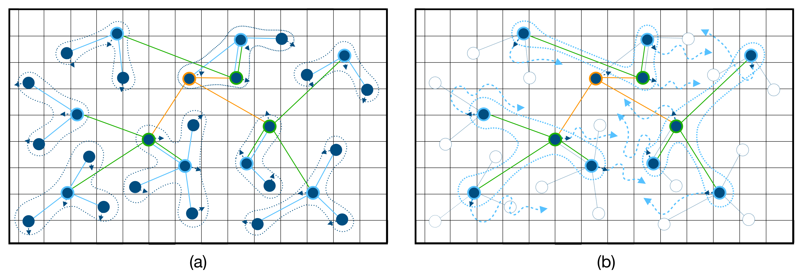
4.3. Hierarchical Multi-Level Clustering

Single-level clustering permits agents to only communicate with cluster-members, preventing inter-cluster communication. To allow this capability, level-1 cluster-heads can form level-2 clusters and elect level-2 cluster heads, continuing the process for higher levels until all robots are united under one hierarchical multi-level clustering (MLC) tree, as depicted in Figure 6.

A completely unique set of challenges emerges in MLC. Strictly speaking, the levels are not independent; processes that occur in lower-level clusters such as evictions, leader elections, cluster merges and splits, also change the membership of higher-level clusters. Regardless of the activity in higher or lower levels, it is generally desirable that all agents remain responsive to the agents in their vicinity and protected from the overhead of the full tree. Two principles aid in that endeavor: first, every cluster-head must belong to a level-1 cluster, and second, every robot must only be the head of one cluster.

To isolate higher-level clusters from the activity in lower-levels, each level-k cluster is associated with a token that points to the tokens of its level $k-1$ cluster-members and the token of its level $k+1$ cluster-head. Any membership changes to a level-k cluster can then be executed by token transfers and pointer modifications at levels $k-1$ and $k+1$. It is useful to see examples of token behavior in some basic cluster operations.

(O1)

Cluster-Head Reassignment: Sometimes a designated cluster-head is no longer suitable for the role. This occurs when another member is closer to the centroid of the cluster, or the cluster-head “despawns” (i.e., powers-down or self-disables). Prior to the trigger-event, the cluster-head transfers the cluster token (and the associated responsibilities) to the member closest to the centroid.

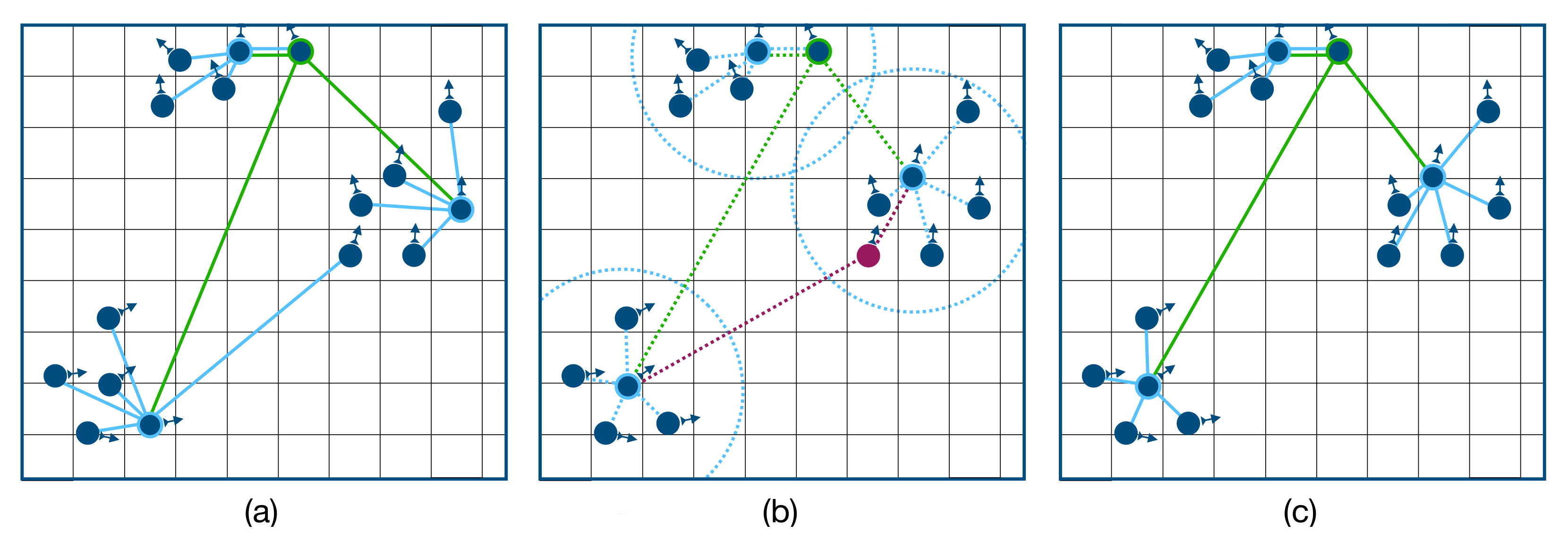
(O2)

Member Transfer: An agent may drift closer to the centroid of another cluster. The “old” cluster-head then initiates a transfer to the new cluster by alerting the higher-level head of the sub-tree. Upon approval, the old token deletes its pointers to the departing agent. The new token adds pointers to the joining agent, which does the same in reciprocity, as depicted in Figure 7.

(O3)

Cluster Split: Level-k clusters with sizes that exceed a certain threshold may split in two. The level-$k+1$ cluster-head creates a new level-k token and designates the new level-k cluster-head as an “idle” member (an agent in the sub-tree that is not the head of any cluster) closest to the centroid. The new cluster includes all members of the old cluster closest to the new cluster-head. The token pointers are adjusted appropriately.

(O4)

Cluster Assimilation: Clusters can also shrink when their members leave or de-spawn. If a level-k cluster-size falls below a threshold, the level-k cluster-head initiates an assimilation request, in which the head of the subtree moves the members to the closest level-k clusters. The token of the old level-k cluster is then destroyed.

(O5)

Boss Demotion: As the system approaches the end of its operating lifetime, agents de-spawn faster than they re-spawn. The MLC tree then shrinks until the head of the tree, (i.e., the boss) has only one member in its cluster. The boss destroys its token to make this member the new boss and eliminate the superfluous extra level.

A universal implementation of MLC does not exist, but the operations above describe a general architecture [52]. MLC protocols can also serve as reliable underlays for high-rate shortest-path protocols with less reliable links. The underlay delivers the low-bandwidth control packets of the overlay while the overlay delivers the high-bandwidth data packets of the application layer [53].

4.4. Belief Propagation in Multi-Level Clustering

The previous discussion of MLC focused on the need for reliable communication in multi-robot networks, where safe collision-free operation is of paramount importance. However, the wireless medium itself is subject to fundamental scaling laws that bound the total throughput as the size of the network (i.e., the number of nodes) grows to infinity [36]. Wireless scaling has been studied extensively in the literature [54,55]. For convenience, let $n:=\left|\mathcal{N}\right|$ denote the number of nodes in the network. The sharpest results so far show the total throughput $T\left(n\right)$ satisfies:

$$\begin{array}{c}\hfill T\left(n\right)\le K(ϵ)n^{1-ϵ},\end{array}$$

(19)

where $K(ϵ)$ is function of $ϵ$. Moreover,

$$\begin{array}{c}\hfill \underset{ϵ\to 0}{lim}K(ϵ)n^{1-ϵ}=0.\end{array}$$

(20)

The implication of (19) and (20) is that the rate per-node goes to zero as the number of nodes becomes large. Therefore a communication policy in which nodes transmit uncompressed data is not scaleable in multi-agent networks. MLC is necessary because it matches the locally interactive structure of the global state to the network capabilities (bounded by (19)).

Each agent has a “belief”, a probabilistic estimate of interest-point locations in the grid. Beliefs play a key role in the POMDP framework; the value function depends on the beliefs over states and not the states themselves. In multi-agent systems, the beliefs of the agent may differ. Each agent is relatively confident about the interest-point locations in its vicinity, and perhaps less so of those in the remote regions; those in the vicinity are observed directly, whereas those further way are relayed through the communication network. Since the global state-space has soft locally interactive structure (Section 3), the robots need not have the same beliefs to collectively maximize the interest-points visited over the operating lifetime. It is this freedom that allows the system to satisfy (19).

The MLC tree defines a mechanism for belief sharing that conforms to the scaling laws in (19). The level-k cluster-heads aggregate the beliefs of their cluster-members into a single belief and send this belief to their level-$k+1$ cluster-heads. In return they receive beliefs from outside of the sub-tree, and forward them down to their members. Every level of the MLC adds another layer of compression to ensure the total throughput does not exceed (19).

To make this more precise, let $b\left(i\right)$ and $s\left(i\right)$ denote the belief and local state of agent i respectively. Assume this agent is a cluster-head and let $\mathrm{level}\left(i\right)$ denote the cluster level. Let $M\left(i\right)\subseteq \mathcal{N}$ denote the members of the cluster where $\mathcal{N}$ is the set of agents. Let c denote the compression factor. The compression algorithm satisfies the following recursion:

$$\begin{array}{cc}\hfill b\left(i\right)& =\left\{\begin{array}{cc}\frac{1}{c}\sum _{j\in M\left(i\right)}b\left(j\right),\hfill & \mathrm{level}\left(i\right)>0,\hfill \\ s\left(i\right),\hfill & \mathrm{level}\left(i\right)=0,\hfill \end{array}\right.\hfill \end{array}$$

(21)

where the sum ${\sum }_{k\in M\left(j\right)}b\left(k\right)$ denotes the belief aggregation performed by agent j.

Belief propagation in general multi-agent networks has also been studied in the literature [56,57]. One of the main challenges is preventing old beliefs from contaminating new beliefs, which occurs when there are cycles in the network that propagate beliefs indefinitely. Tree-structured networks (like MLC) have no cycles.

The successful propagation of beliefs does not in itself guarantee optimal system operation. Agents must still collectively “sample” the global state in search of interest-points by visiting all regions sufficiently often. The process of exploration continues until the system learns the interest-point dynamics. During this process, some agents may forgo visiting the areas that previously had many interest-points; agents choose to explore rather than exploit existing knowledge. The “exploration vs exploitation” trade-off is a fundamental area of study in RL and still an active area of research.

5. A Proposed Control/Communication Architecture for Multi-Agent Systems

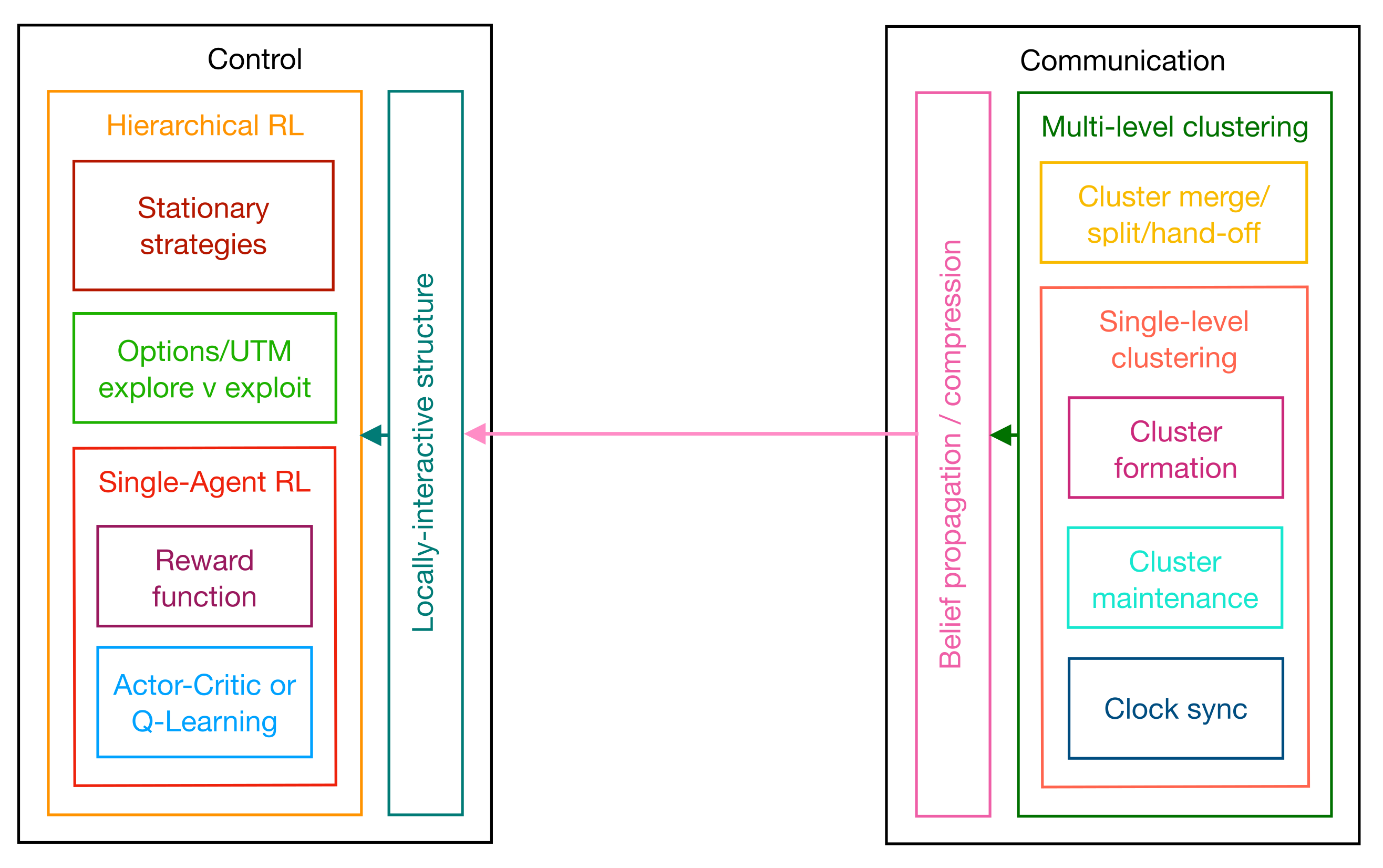
The goal of this paper was to show that a broad selection of work in the literature fits into a proposed control/communication “architecture”; an organized set of interacting, independent modules. This architecture is depicted in Figure 8.

A “module” defines an interface with some concrete functionality, while the “interface” specifies the inputs and outputs of the desired task. The implementation or mechanism used to execute the task is not specified by an architecture, the expectation being that every implementation is eventually made obsolete by advances in technology. An architecture, by contrast, describes something more resilient and rooted in fundamental constraints of the system itself, constraints that do not change with technology but describe the limits of what technology can do. In the proposed architecture, these constraints are the complexity and network capacity of multi-agent systems. The modules in Figure 8 are less formal and loosely refer to common tasks appearing repeatedly in the literature.

Figure 8 highlights a duality between the control and communication components of the architecture. Both components start with a single-agent module (an RL agent or a cluster) and build a multi-level hierarchy over that module. On the control side, the sub-modules of an agent include the reward function and the mechanism for finding optimal primitive policies (i.e., actor-critic or Q-learning). The outer module includes the single-agent sub-module as well as two sub-modules required in hierarchical multi-agent reinforcement learning. The first ensures the system remains stationary over the option-space, and the second determines the structure of the option-space. The latter, by implication, also includes traffic management capabilities and an exploration/exploitation trade-off.

The communication side mirrors this progression, from single-level clusters to hierarchical multi-level clustering trees. Single-level clusters include sub-modules for cluster formation, cluster maintenance, and clock synchronization, whereas multi-level clusters implement the merge, split, and hand-off functionality. Multi-level clustering disseminates local state information to all of the agents in the form of “beliefs”. The mechanism for belief “sharing” or “propagation” includes some form of data compression.

Beliefs shared through the clustering tree must conform to the locally interactive structure of the state space; agents should only exert higher-order influence on any remote agent receiving their compressed and aggregated local states. The module that interprets locally interactive structure on the control side receives the beliefs shared from the communication side. This module constructs a compressed global state for each agent centered at the agent, and feeds this reconstructed state into the agents’ control policy, connecting the control and communication components.

Each module in the architecture has received attention in the literature, and there is no single implementation that supersedes all others. Incremental improvements at the modular level will likely continue well into the future, but there are fundamental constraints on capacity and complexity that can never be exceeded. Twin pillars of the proposed architecture (i.e., locally interactive structure and multi-level clustering) cater precisely to these constraints. Locally interactive structure keeps complexity in check, by settling for approximately optimal performance (13) and compressing the state-space (12). Multi-level clustering satisfies throughput constraints by compressing the beliefs hierarchically (21). These operations are mutually beneficial and motivate a yet-to-be-made proof-of-concept for the full architecture.

A drawback of deep RL is that the learning process does not always find the optimal policy ${\pi }^{*}\left(s\right)$. Deep RL relies on neural networks to approximate the value $V_{\pi }^{*}\left(s\right)$ of ${\pi }^{*}\left(s\right)$, and these networks converge to local maxima via stochastic gradient descent. Local maxima are generally not globally optimal. The optimal trajectories can be computed by solving an extended version of the TSP, but such solutions are complex and do not scale in the number of agents. An alternative is to use a lower-complexity upper-bound on $V_{\pi }^{*}\left(s\right)$ to measure how far the computed policy is from the optimal in the worst case. One such upper-bound was derived in (15)–(18).

5.1. Multi-Agent Coordination and Communication in the Literature

Despite the absence of a universally accepted architecture, multi-agent systems have received sustained attention in the literature. Usually the scope of work falls within individual modules in Figure 8. There have been studies that explore ways of disseminating the minimally required local state information for global coordination [9,58]. To achieve any coordination, global tasks must be converted into individual local tasks [59,60]. The reverse approach is also of interest; inferring the global effect of local controllers in robot swarms [61]. The problem of designing multi-agent controllers is still unresolved. Some approaches rely on factoring “Partially Observable MDPs” or POMDPs [10]. Others use evolutionary methods to weed out “unfit” controllers with fitness functions [60,62]. The promise of deep RL for multi-agent control appears in recent surveys [63]. The closest realization of the architecture in Figure 8 appears in [1]. The local controllers in [1] are largely independent but include some nearest-neighbor interaction.

5.2. Developing a Proof-Of-Concept: A Structured Approach

The architecture in Figure 8 depicts a plausible strategy for the multi-agent tracking problem, based on approaches to some of the sub-problems in the literature. A proof-of-concept/implementation for the whole architecture has yet to appear, but the goal of this paper is to motivate efforts to that end. The following section outlines a structured approach towards a possible implementation, using insights from the authors’ experiences in this space.

The main objective of this architecture is to support a scaleable solution; one that enables “approximately” optimal tracking with arbitrarily many agents. If we assume all agents have access to full state information, the complexity of multi-agent reinforcement learning still grows exponentially in the number of agents (without any mitigating strategies). It is natural to address this bottleneck first and progressively relax each assumption, adding more modules in the architecture until reaching a fully decentralized solution.

Some reasonable guidelines define an approach towards a proof-of-concept. The first is to keep the action-space small; the complexity of a primitive space (i.e., “up”, “down”, “left”, “right”), still grows exponentially in the number of agents and remains unsolved. Once a solution for the primitive space is found, more complex aerodynamic actions can be considered. The next is to start with basic RL before proceeding to deep RL. The former works with the “raw” Q-tables $Q_{\pi }(s,\mathbf{a})$ and does not include any function approximation. Since the number of entries in the table (state-action pairs) grows exponentially in the number of agents and interest-points, basic RL is limited to small numbers of agents and interest-points and grid sizes. Nevertheless, it is useful to understand the reward function in small dimensions, for approximation in large dimensions with neural networks. The overarching principle is to extrapolate more complex behavior of the system from its simpler forms, proceeding in stages, gently increasing the complexity of the system while adding forensic tools in software to help identify if and where divergence occurs.

We propose a set of milestones consistent with the guidelines above, that define a structured approach towards a proof-of-concept. While there is no one fixed set of milestones, the approach we propose may inspire others.

(M1)

The Single-Agent, Stationary Interest-Points Scenario. The agent visits a sequence of stationary interest-points on a two-dimensional grid, using the shortest path. Training is performed with basic RL, under the assumption the agent has full-state state information.

For a single stationary interest-point, this scenario reduces to the grid-world problem, a well-known example in RL. The grid-world problem becomes much harder with two interest-points. A scenario with multiple interest-points corresponds to the TSP, where the optimal solution requires an exhaustive search over all possible trajectories. The next section will explain why this milestone, even with two interest-points, benefits from advanced strategies like hierarchical RL.

(M2)

The Multi-Agent, Stationary Interest-Points Scenario. A system of multiple agents finds an approximately optimal set of trajectories that visit stationary interest-points on a two-dimensional grid. Training is performed using basic RL under the assumption that each agent now observes the full system state. This milestone incorporates macro-actions (i.e., “Agents 1, 4, and 5 move to sub-region A”) to keep the distribution of agents and interest-points in equilibrium. It focuses on policies reasonably achievable by training Q-tables, excluding moving interest-points and the large scale activity of many agents (i.e., dynamic sky-way networks).

(M3)

The Multi-Agent Mobile Interest-Points Scenario. A system of agents tracks moving interest-points on a two-dimensional grid. Training is performed using deep RL, under the assumption that each agent observes the full system state. The objective is to verify that neural networks can model tracking policies for various interest-point trajectories. To achieve this milestone, it is logical to start with one agent and one stationary interest-point, where the reward function has a simple discernible structure. The next step is to let the interest-point move predictably (i.e., around a circle at constant velocity). Next, add two interest-points. Then incrementally increase the complexity of the system, verifying at each stage that the extra complexity is captured in training.

(M4)

The Scaleable Multi-Agent Scenario. The system maintains approximately optimal performance as the number of agents grows large. Training is performed using deep RL, but each agent relies on its local state and a compressed/aggregated version of the global state space. Macro-actions now include unmanned traffic management (UTM) to support large-scale high-traffic drone transportation. The “dynamic sky-way network” redistributes agents over the grid to keep the distribution of agents and interest-points in equilibrium, and consists of a few high-throughput airways for long distances and many low-throughput airways for finer redistribution over short distances. The shape of the network adapts to the distribution of interest-points in real-time. Agents collectively determine the trajectories of airways that traverse their respective sub-regions.

(M5)

The Multi-Agent Multi-Level Clustering Scenario. Agents rely on a multi-level clustering scheme to disseminate/aggregate their local state information and infer a common view of the global state. Cluster-heads compress state information to ensure the information throughput has sub-linear scaling. Each cluster organizes local activity and cooperates with higher-level clusters to ensure the system behaves in a coordinated manner. The system supports essential distributed tasks like cluster-formation, cluster-maintenance, and synchronization. The clustering algorithm is fully integrated into the RL training process developed in the previous milestones.

5.3. A Case-Study of Milestone M1

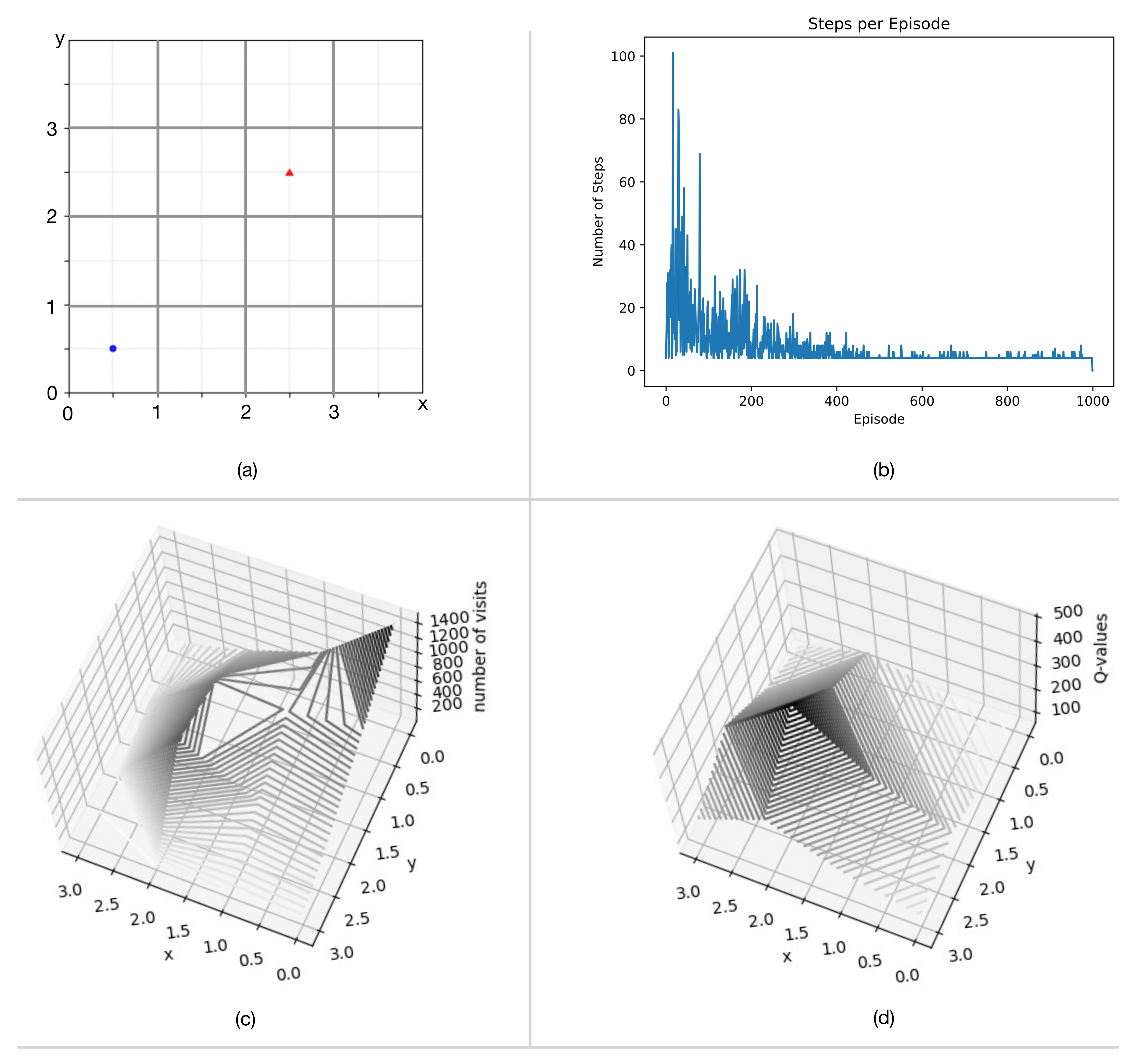
To further explore the process of developing a proof-of-concept, we offer a case-study of milestone M1. First, we introduce a system with one agent and one stationary interest-point, then consider some challenges in the extension to two stationary interest-points. The system, depicted in its initial state in Figure 9a, is a grid of side-length 4. The agent objective is to find the shortest path (defined by four primitive actions {“up”, “down”, “left”, “right”}) from the agent to the interest-point. By inspection, shortest paths have length 4 and are thus simple to verify.

The scheme used in this case-study employs basic q-learning (i.e., q-tables). For the single interest-point scenario, the reward r given to each state-action pair $(s,a)$ is $r=500$ if the positions of the agent and interest-point coincide, $r=-10$ if the action drives the agent into the boundary, and $r=-1$ otherwise. The hyperparameters which determine the update rule are $\alpha =0.3$, $\gamma =0.6$, and $ϵ=0.1$. The $ϵ$-greedy policy which samples the state space selects a “greedy” or “exploitative” action $a^{*}={max}_{a}q(s,a)$ with probability $1-ϵ$ and a random exploratory action (uniformly from one of the four primitive choices) with probability $ϵ$. After each step, the table of q-values (i.e., the value of each state-action pair) is updated according to the following rule: $q(s,a)\leftarrow q(s,a)+\alpha (r+\gamma {max}_{a}q(s^{\prime },a)-q(s,a))$. Recall that $s^{\prime }$ is the state outcome after the agent performs action a in state s. The update rule “boot-straps” old estimates of the q-values into new estimates. The training episode terminates when the positions of the agent and interest-point coincide. Figure 9 shows the outcome after 1000 training episodes.

Figure 9b shows the number of steps per training episode converges approximately to 4 (which is the length of the shortest trajectory). This convergence is also evident in Figure 9c which shows the total number of visits to each cell over all training episodes. The starting point at position $(0,0)$ has the most visits. The intermediate positions on the shortest trajectories between $(0,0)$ and $(2,2)$ are also visible in Figure 9c. Positions outside these trajectories are visited rarely indicating that the $ϵ$-greedy policy converges to the optimal one.

Figure 9d shows the maximum q-value ${max}_{a}q(s,a)$ for each cell. The q-value peaks at position $(2,2)$ and a value of 500, because the agent at this position coincides with the interest-point. The surrounding cells include the expectation of this discounted future reward, yielding a pyramid shape. The $ϵ$-greedy policy uses the q-values to determine the appropriate action in each state, choosing actions that maximize the expected return. This policy corresponds to the shortest path between the agent and interest-point.

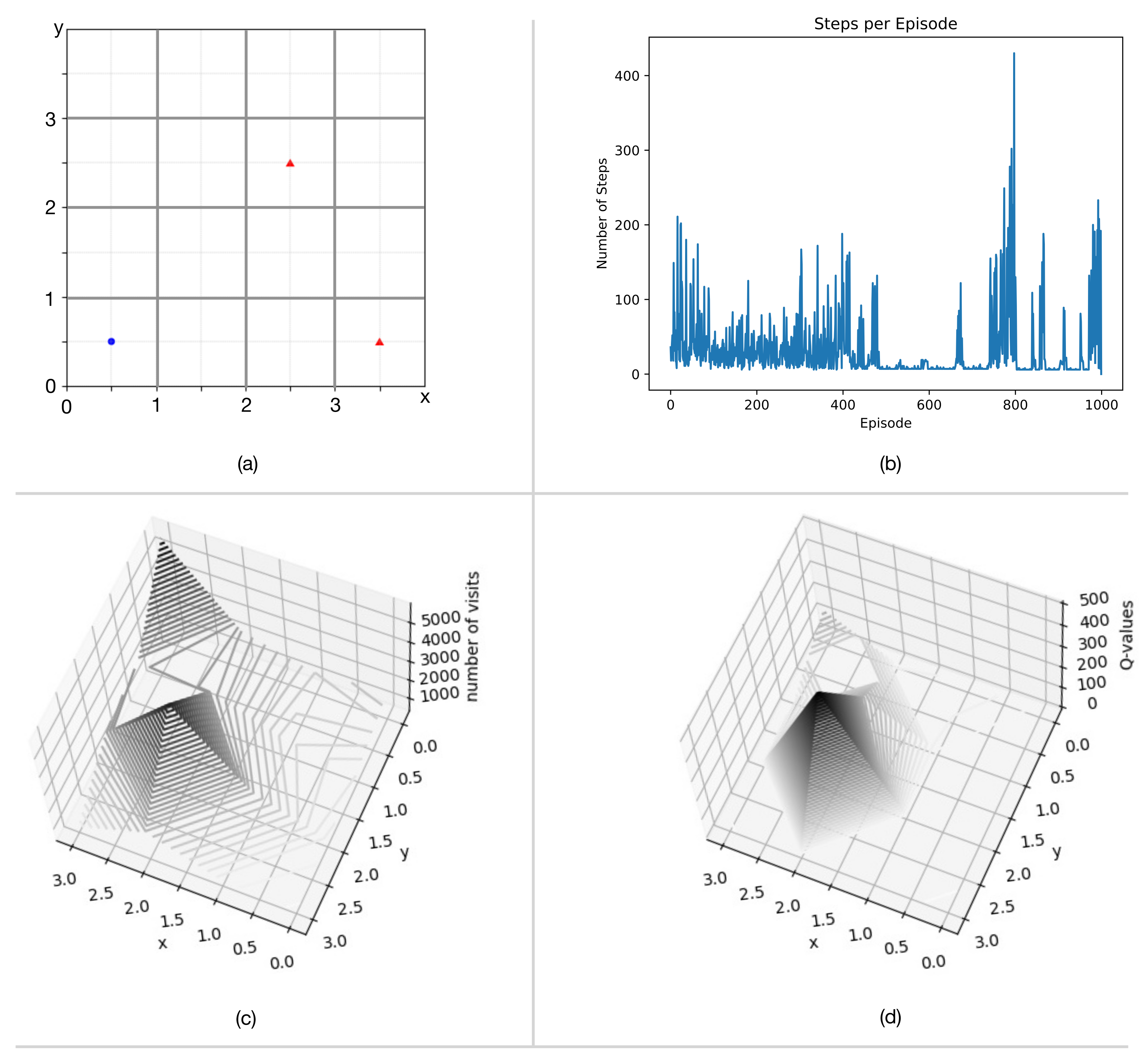
Now we add an additional stationary interest-point to the system and observe the effect on the learning process. The reward function with multiple interest-points is modified to assign $r=500$ for every un-visited interest-point. The hyper-parameters and update rule are the same as before. Figure 10 shows the results after 1000 training episodes.

Figure 10b shows the training process does not converge; the number of steps per episode oscillates between periods of stability and instability. Figure 10c,d provide some insight into this undesirable behavior. Cells with interest-points receive a larger share of visits compared to other cells, as evident in Figure 10c. However, visits to the first of the two interest-points (cell (3,0)) do not seem to accrue much reward in Figure 10d; the q-values acquired in training diverge from the “true” q-values. This occurs because the first visit to an interest-point accrues a reward of $r=500$, but the $ϵ$-greedy learning policy keeps the agent in the vicinity of the interest-point. Subsequent visits to this interest-point accrue negative reward (since it has already been visited), which reduces the value of the cell. Eventually this cell loses most of its value, which under the $ϵ$-greedy policy, releases the agent to explore other cells.

The true q-function resembles a two-stage pyramid or a “ziggurat”. The previous discussion explains why $ϵ$-greedy policies with one-step returns cannot accurately estimate multi-stage q-functions. This problem is partially mitigated by using multi-step returns in the update (instead of one-step returns), but emerges again if the number of interest-points or grid dimensions increase. A more permanent solution is to hierarchically structure the action-space into primitive actions and macro-actions (i.e., “move agent 1 to interest-point 1” and “move agent 1 to interest-point 2”). The training process then determines the order of visitations and the shortest path to each interest-point from the current position of the agent.

The two-stage hierarchical action-space is one possible way of completing M1. Mobile interest-points require more advanced techniques outlined in Section 5.2. Figure 9 and Figure 10 demonstrate the forensic analysis needed to incorporate the extra complexity of each new milestone.

6. Conclusions

This paper highlights possibilities for a unified control/communication architecture in multi-agent tracking systems. The main components of this architecture, locally interactive state spaces and multi-level clustering, address fundamental limitations in the control and communication spheres. An architecture only gives an outline of a solution and omits (by design) the details of any implementation. From the reward function, to options, the training algorithm, the performance metrics, the rules for clustering, and belief aggregation, all of these details require further investigation, development, testing, and integration. The case-study included in this survey provides some perspective of the work required to develop a proof-of-concept for the overall architecture.