
Ground Vibration Testing of a Flexible Wing: A Benchmark and Case Study

 ,
,  , , and
Abstract
:1. Introduction
2. Materials and Methods
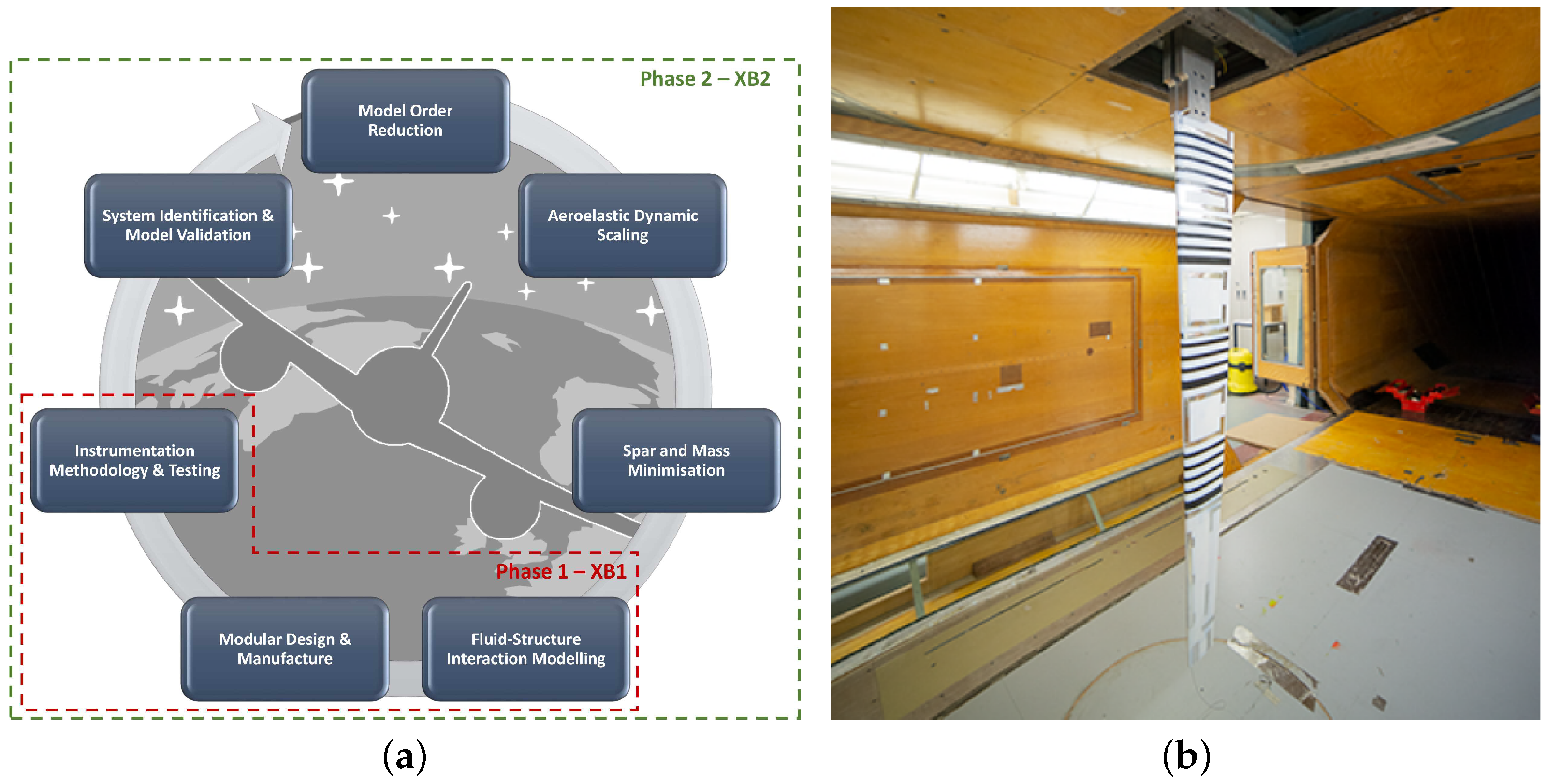
2.1. The XB-2 High Aspect Ratio Wing
2.1.1. The Spars
2.1.2. The Tube
2.1.3. The Skin
2.2. Theoretical and Numerical Predictions
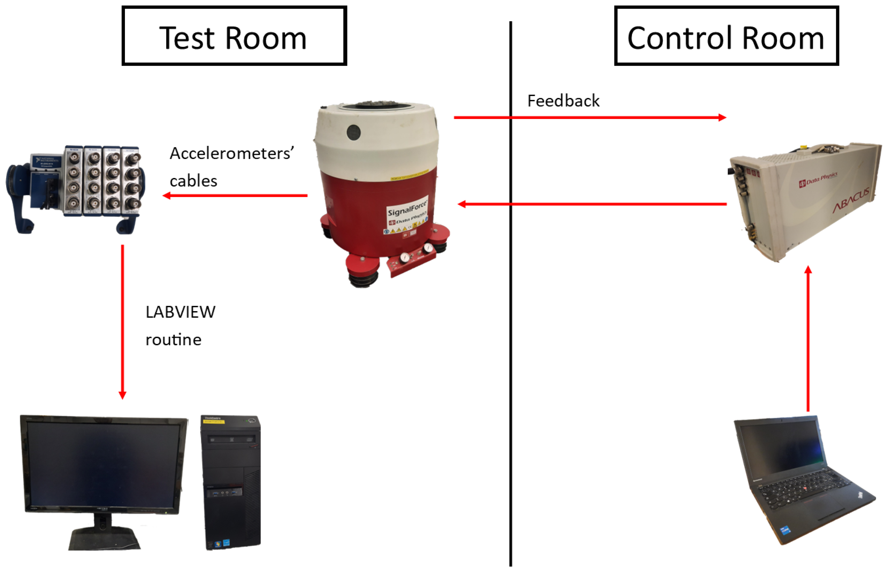
2.3. Experimental Setup
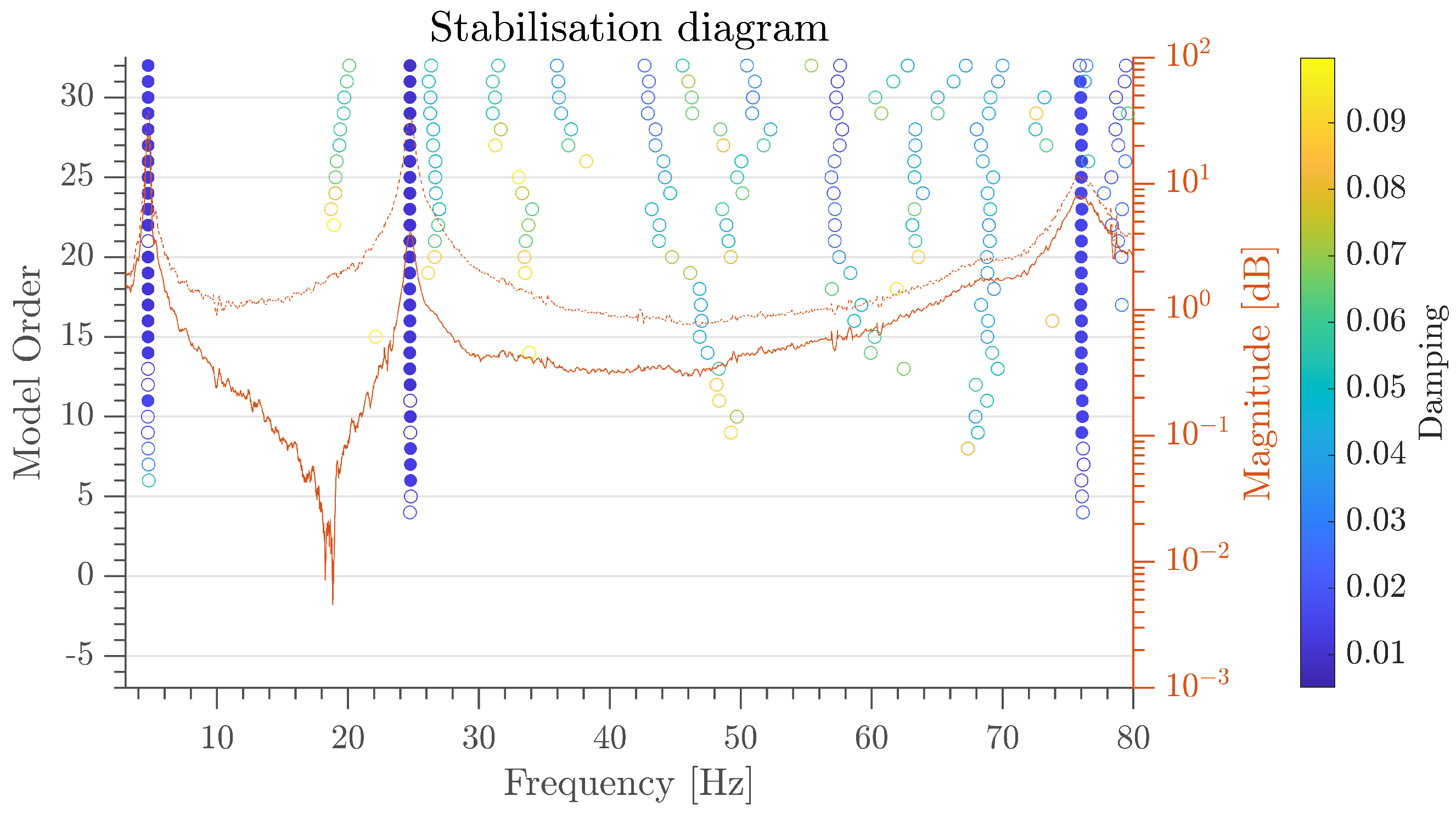
2.4. Data Processing and Identification
3. Results
3.1. Twin Spar
3.2. Main Spar
3.3. Spar and Tube
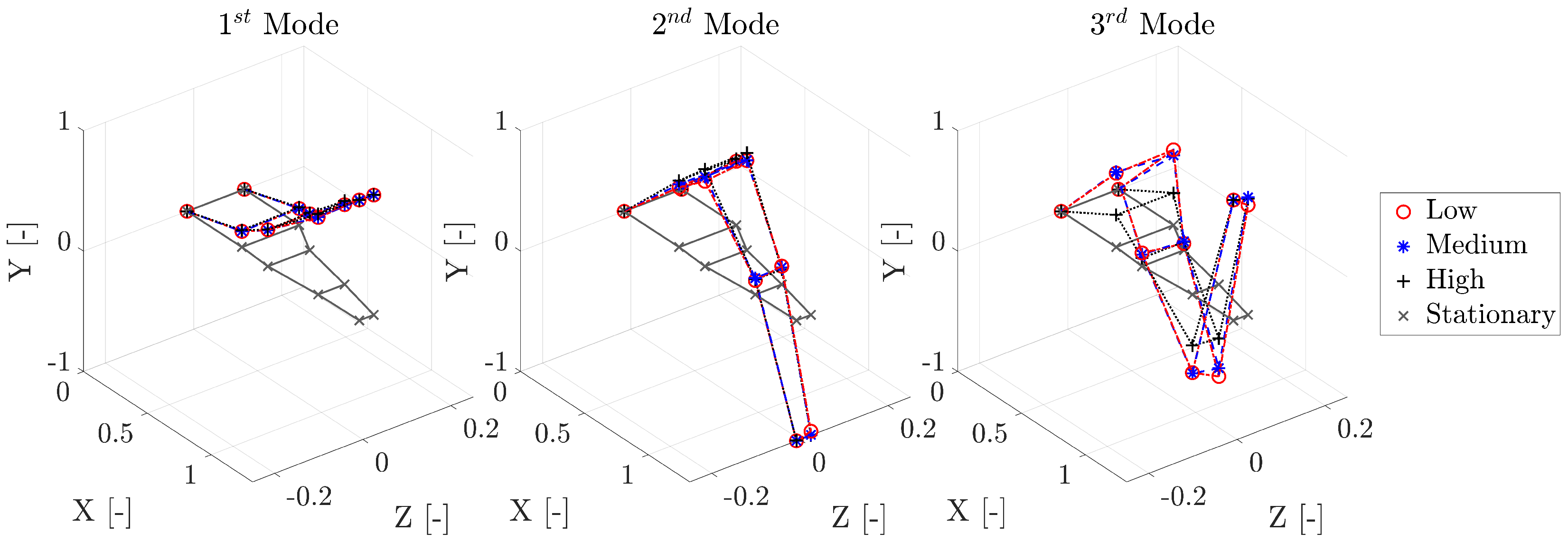
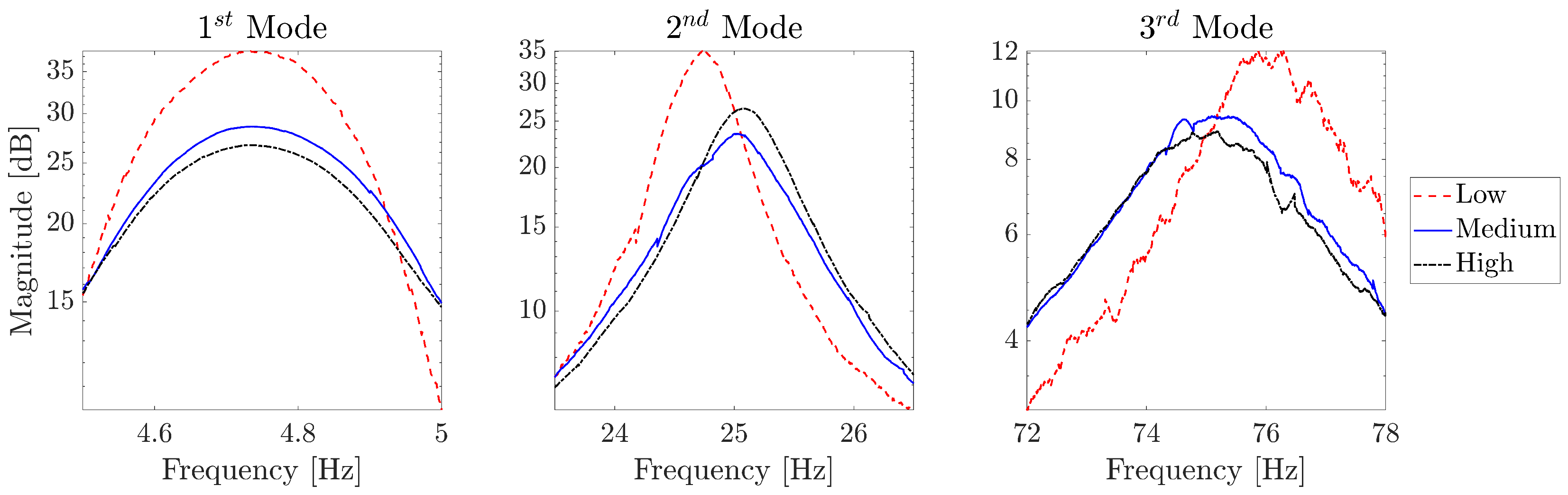
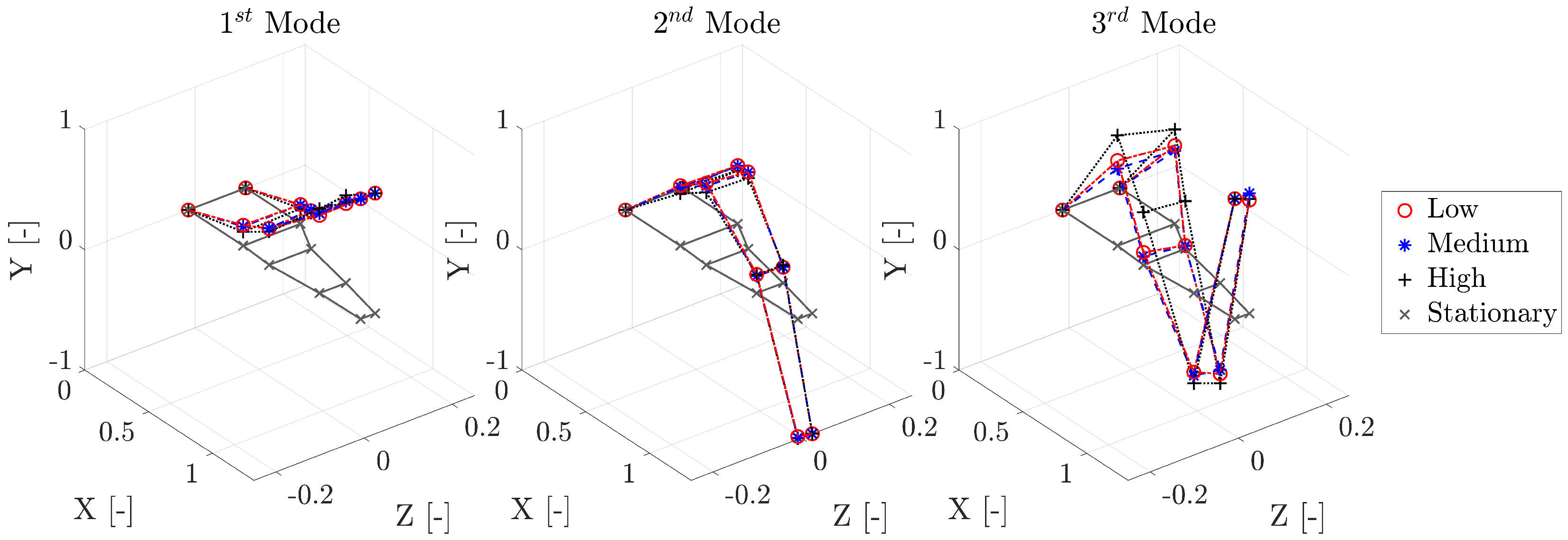
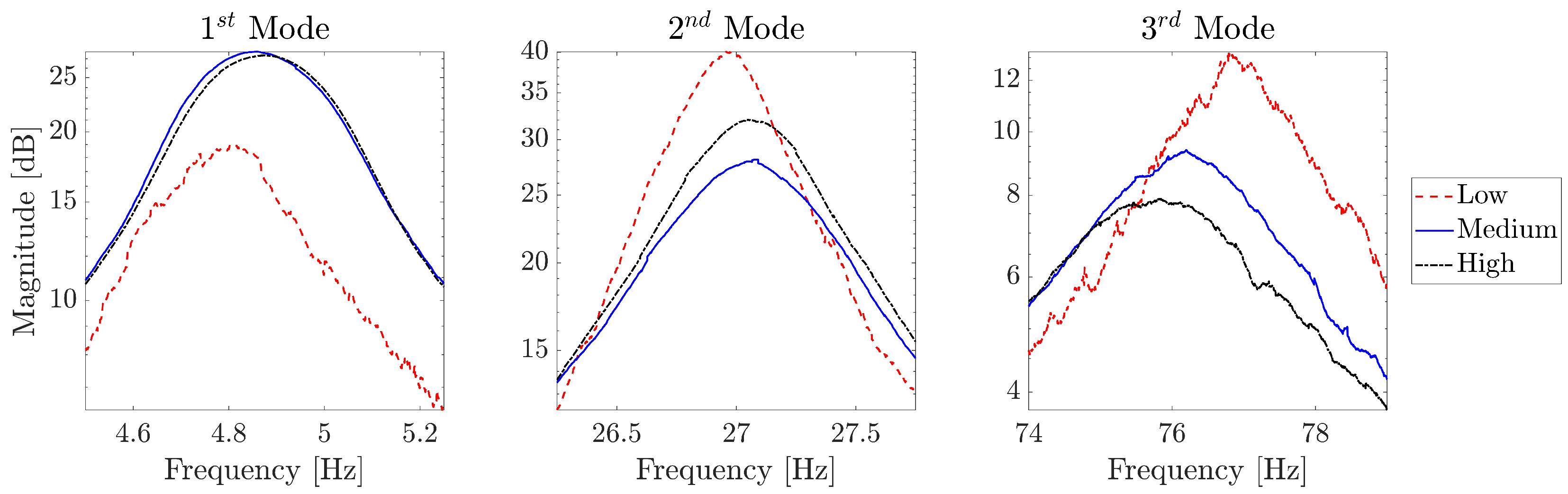
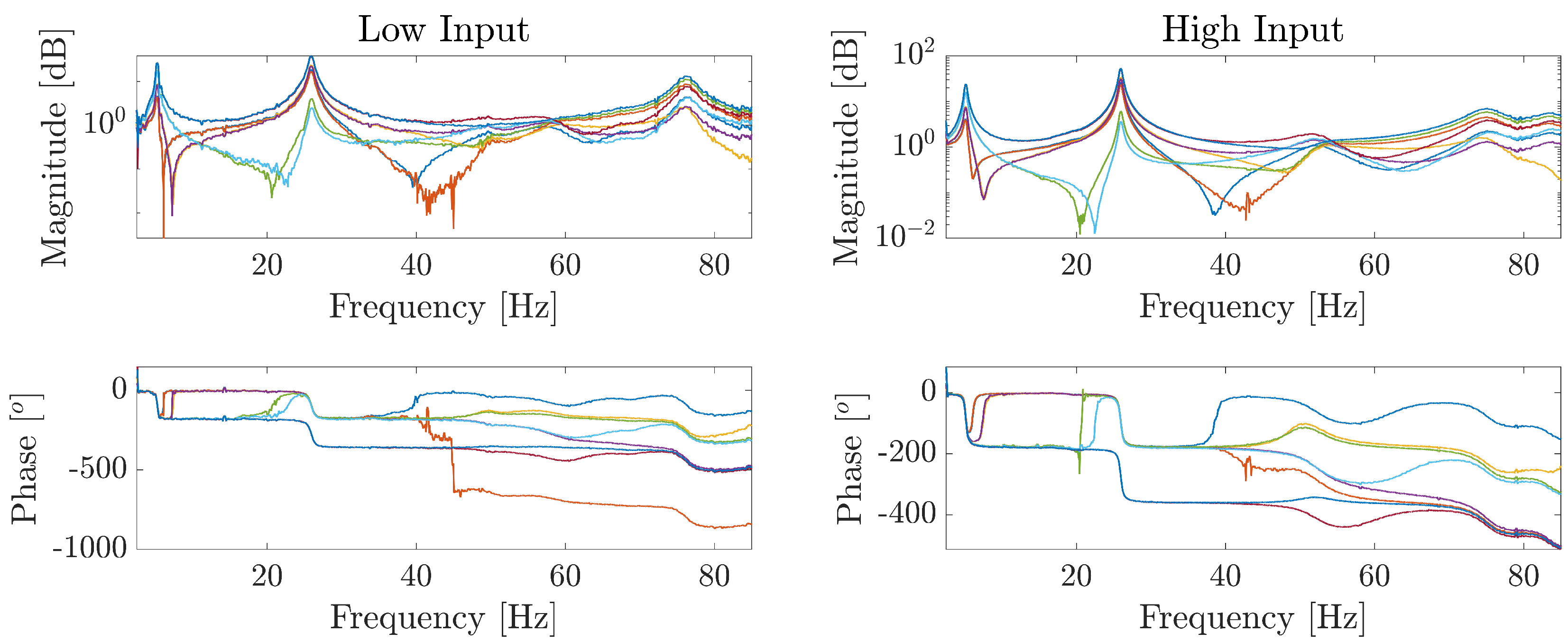
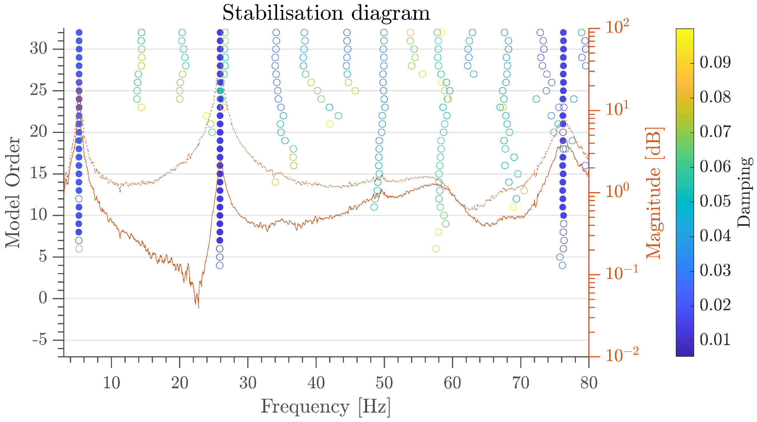
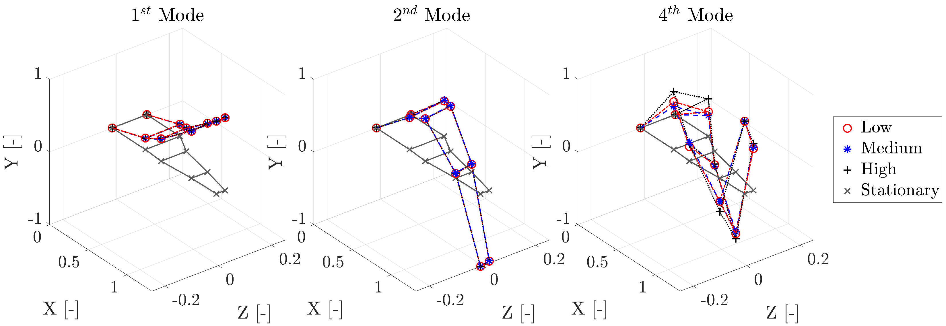
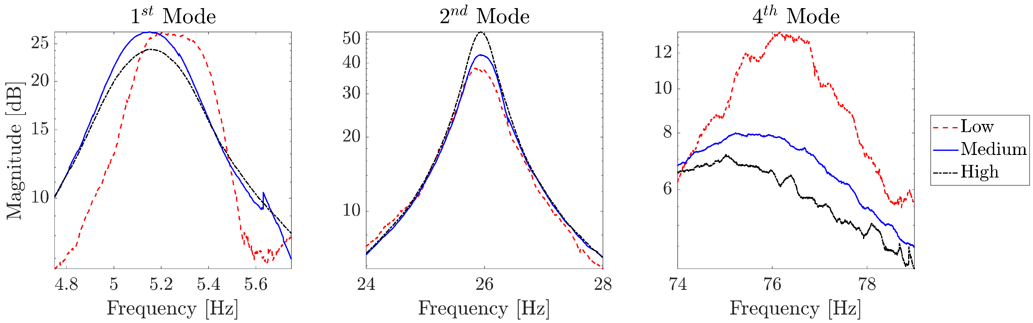
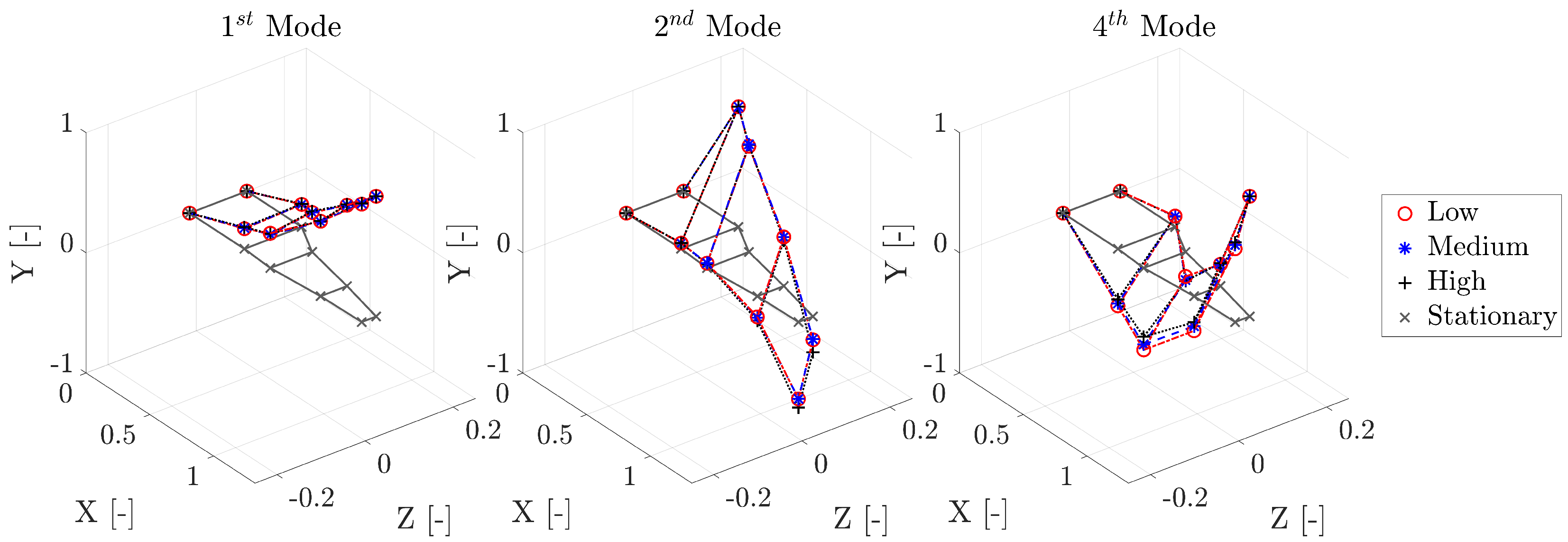
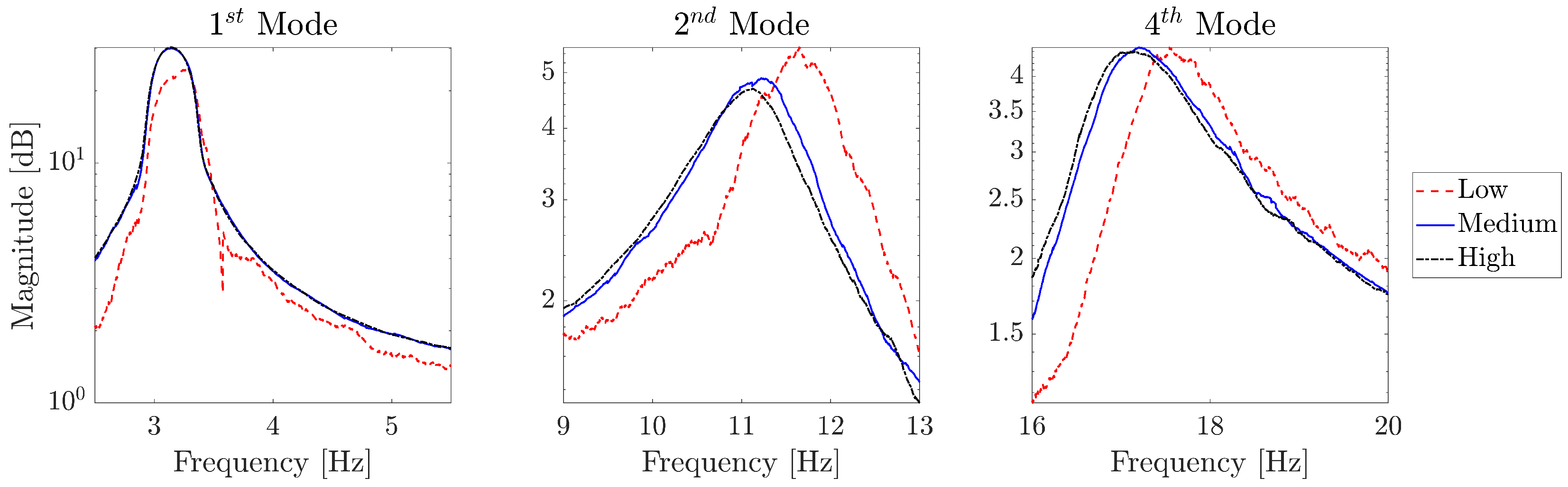
3.4. Full Wing
4. Discussion
4.1. Twin Spar
4.2. Main Spar
4.3. Spar and Tube
4.4. Full Wing
4.5. Overall Considerations
5. Conclusions
Author Contributions
Funding
Institutional Review Board Statement
Informed Consent Statement
Data Availability Statement
Acknowledgments
Conflicts of Interest
Appendix A. Identification Data

| Low Input | Medium Input | High Input | |||||||
|---|---|---|---|---|---|---|---|---|---|
| Mode | 1st | 2nd | 3rd | 1st | 2nd | 3rd | 1st | 2nd | 3rd |
| 4.731 | 24.733 | 75.939 | 4.742 | 25.029 | 75.124 | 4.738 | 25.087 | 75.106 | |
| 0.013 | 0.010 | 0.017 | 0.027 | 0.021 | 0.021 | 0.029 | 0.016 | 0.022 | |
| 0.137 | 0.531 | 0.626 | 0.138 | 0.525 | 0.580 | 0.149 | 0.550 | 0.268 | |
| 0.131 | 0.497 | 0.614 | 0.132 | 0.521 | 0.624 | 0.141 | 0.553 | 0.267 | |
| 0.303 | 0.744 | 0.056 | 0.303 | 0.746 | 0.074 | 0.309 | 0.809 | 0.069 | |
| 0.303 | 0.706 | 0.111 | 0.300 | 0.743 | 0.098 | 0.306 | 0.806 | 0.069 | |
| 0.662 | 0.152 | −0.765 | 0.664 | 0.142 | −0.693 | 0.664 | 0.123 | −0.449 | |
| 0.640 | 0.117 | −0.649 | 0.642 | 0.137 | −0.656 | 0.669 | 0.126 | −0.423 | |
| 0.995 | −0.967 | 0.911 | 0.996 | −0.997 | 0.977 | 0.9986 | −1 | 0.965 | |
| 1 | −1 | 1 | 1 | −1 | 1 | 1 | −0.997 | 1 | |
| Low Input | Medium Input | High Input | |||||||
|---|---|---|---|---|---|---|---|---|---|
| Mode | 1st | 2nd | 3rd | 1st | 2nd | 3rd | 1st | 2nd | 3rd |
| 4.855 | 26.966 | 76.851 | 4.866 | 27.050 | 76.195 | 4.876 | 27.057 | 75.805 | |
| 0.033 | 0.010 | 0.014 | 0.029 | 0.016 | 0.020 | 0.029 | 0.014 | 0.022 | |
| 0.159 | 0.484 | 0.650 | 0.157 | 0.481 | 0.607 | 0.126 | 0.442 | 0.784 | |
| 0.171 | 0.500 | 0.708 | 0.160 | 0.487 | 0.641 | 0.116 | 0.435 | 0.918 | |
| 0.317 | 0.639 | 0.028 | 0.325 | 0.637 | 0.025 | 0.297 | 0.587 | 0.397 | |
| 0.302 | 0.680 | 0.104 | 0.306 | 0.656 | 0.071 | 0.277 | 0.603 | 0.438 | |
| 0.660 | 0.131 | −0.755 | 0.679 | 0.133 | −0.722 | 0.728 | 0.148 | −0.834 | |
| 0.646 | 0.156 | −0.656 | 0.663 | 0.144 | −0.686 | 0.702 | 0.153 | −0.749 | |
| 1 | −1 | 0.942 | 1 | −1 | 0.999 | 1 | −1 | 0.951 | |
| 0.999 | −0.977 | 1 | 0.999 | −0.988 | 1 | 0.995 | −0.992 | 1 | |
| Low Input | Medium Input | High Input | |||||||
|---|---|---|---|---|---|---|---|---|---|
| Mode | 1st | 2nd | 3rd | 1st | 2nd | 3rd | 1st | 2nd | 3rd |
| 5.252 | 25.933 | 76.242 | 5.151 | 25.958 | 75.770 | 5.163 | 25.941 | 75.135 | |
| 0.022 | 0.014 | 0.017 | 0.030 | 0.011 | 0.034 | 0.036 | 0.010 | 0.034 | |
| 0.165 | 0.486 | 0.337 | 0.161 | 0.494 | 0.286 | 0.163 | 0.494 | 0.515 | |
| 0.158 | 0.439 | 0.658 | 0.153 | 0.441 | 0.595 | 0.156 | 0.440 | 0.798 | |
| 0.323 | 0.621 | −0.185 | 0.318 | 0.631 | −0.205 | 0.322 | 0.630 | −0.173 | |
| 0.307 | 0.584 | 0.199 | 0.301 | 0.587 | 0.257 | 0.306 | 0.585 | 0.232 | |
| 0.672 | 0.107 | −0.849 | 0.662 | 0.116 | −0.823 | 0.672 | 0.112 | −0.918 | |
| 0.646 | 0.0645 | −0.320 | 0.663 | 0.072 | −0.322 | 0.655 | −0.068 | −0.460 | |
| 1 | −0.975 | 0.576 | 0.997 | −0.967 | 0.595 | 0.999 | −0.967 | 0.647 | |
| 0.999 | −1 | 1 | 1 | −1 | 1 | 1 | −1 | 1 | |
| Low Input | Medium Input | High Input | |||||||
|---|---|---|---|---|---|---|---|---|---|
| Mode | 1st | 2nd | 3rd | 1st | 2nd | 3rd | 1st | 2nd | 3rd |
| 3.187 | 11.752 | 17.447 | 3.164 | 11.267 | 17.070 | 3.139 | 11.196 | 16.988 | |
| 0.024 | 0.047 | 0.037 | 0.018 | 0.060 | 0.041 | 0.018 | 0.065 | 0.042 | |
| 0.187 | 1 | 0.090 | 0.187 | 1 | 0.089 | 0.192 | 1 | 0.086 | |
| 0.168 | 0.047 | −0.474 | 0.174 | 0.047 | −0.454 | 0.180 | 0.049 | −0.420 | |
| 0.328 | 0.879 | −0.204 | 0.329 | 0.895 | −0.234 | 0.338 | 0.892 | −0.241 | |
| 0.289 | 0.040 | −0.682 | 0.278 | 0.041 | −0.636 | 0.285 | 0.033 | −0.572 | |
| 0.673 | 0.409 | 0.181 | 0.674 | 0.407 | 0.185 | 0.626 | −0.204 | −0.217 | |
| 0.624 | −0.172 | −0.288 | 0.620 | −0.179 | −0.250 | 0.655 | −0.068 | −0.460 | |
| 1 | −0.195 | 1 | 1 | −0.189 | 1 | 1 | −0.297 | 1 | |
| 0.981 | −0.640 | 0.610 | 0.986 | −0.639 | 0.642 | 0.988 | −0.712 | 0.663 | |
References
- Civera, M.; Zanotti Fragonara, L.; Surace, C. Using video processing for the full-field identification of backbone curves in case of large vibrations. Sensors 2019, 19, 2345. [Google Scholar] [CrossRef] [PubMed] [Green Version]
- Pontillo, A.; Hayes, D.; Dussart, G.X.; Lopez Matos, G.E.; Carrizales, M.A.; Yusuf, S.Y.; Lone, M.M. Flexible high aspect ratio wing: Low cost experimental model and computational framework. In Proceedings of the 2018 AIAA Atmospheric Flight Mechanics Conference, Kissimmee, FL, USA, 8–12 January 2018; American Institute of Aeronautics and Astronautics: Reston, VA, USA, 2018; pp. 1–15. [Google Scholar] [CrossRef] [Green Version]
- Yusuf, S.Y.; Pontillo, A.; Weber, S.; Hayes, D.; Lone, M. Aeroelastic scaling for flexible high aspect ratio wings. In Proceedings of the AIAA Scitech 2019 Forum, San Diego, CA, USA, 3–7 January 2019; American Institute of Aeronautics and Astronautics: Reston, VA, USA, 2019; pp. 1–14. [Google Scholar] [CrossRef] [Green Version]
- Hayes, D.; Pontillo, A.; Yusuf, S.Y.; Lone, M.M.; Whidborne, J. High aspect ratio wing design using the minimum energy destruction principle. In Proceedings of the AIAA Scitech 2019 Forum, San Francisco, CA, USA, 3–7 January 2019; American Institute of Aeronautics and Astronautics: Reston, VA, USA, 2019. [Google Scholar] [CrossRef]
- Pontillo, A. High Aspect Ratio Wings on Commercial Aircraft: A Numerical and Experimental Approach. Ph.D. Thesis, Cranfield University, Cranfield, UK, 2020. [Google Scholar]
- Spitznogle, F.R.; Quazi, A.H. Representation and analysis of time-limited signals using a Complex Exponential algorithm. J. Acoust. Soc. Am. 1970, 47, 1150–1155. [Google Scholar] [CrossRef]
- Spitznogle, F.R.; Barrett, J.M.; Black, C.I.; Ellis, T.W.; LaFuze, W.L. Representation and Analysis of Sonar Signals. Volume I. Improvements in the Complex Exponential Signal Analysis Computational Algorithm; Technical Report; Office of Naval Research-Contract No. NOOO14-69-C0315; Defense Technical Information Center: Fort Belvoir, VA, USA, 1971. [Google Scholar]
- Verhulst, T.; Judt, D.; Lawson, C.; Chung, Y.; Al-Tayawe, O.; Ward, G. Review for State-of-the-Art Health Monitoring Technologies on Airframe Fuel Pumps. Int. J. Progn. Health Manag. 2022, 13, 1–20. [Google Scholar] [CrossRef]
- Rizzo, P.; Enshaeian, A. Challenges in bridge health monitoring: A review. Sensors 2021, 21, 4336. [Google Scholar] [CrossRef] [PubMed]
- Dessena, G.; Civera, M.; Zanotti Fragonara, L.; Ignatyev, D.I.; Whidborne, J.F. A Loewner-based system identification and structural health monitoring approach for mechanical systems. Struct. Health Monit. 2022, 17. [Google Scholar]
- Civera, M.; Mugnaini, V.; Zanotti Fragonara, L. Machine learning-based automatic operational modal analysis: A structural health monitoring application to masonry arch bridges. Struct. Control. Health Monit. 2022, e3028. [Google Scholar] [CrossRef]
- Dessena, G.; Ignatyev, D.I.; Whidborne, J.F.; Zanotti Fragonara, L. A Kriging Approach to Model Updating for Damage Detection. In Proceedings of the EWSHM 2022, Palermo, Italy, 4–7 July 2022; Rizzo, P., Milazzo, A., Eds.; Springer: Cham, Switzerland, 2022. Chapter 26. pp. 245–255. [Google Scholar] [CrossRef]
- De Florio, F. Airworthiness; Elsevier: Amsterdam, The Netherlands, 2011. [Google Scholar] [CrossRef]
- Keane, A.J.; Sóbester, A.; Scanlan, J.P. Small Unmanned Fixed-Wing Aircraft Design; John Wiley & Sons: Chichester, UK, 2017. [Google Scholar] [CrossRef]
- Nöel, J.P.; Renson, L.; Kerschen, G.; Peeters, B.; Manzato, S.; Debille, J. Nonlinear dynamic analysis of an F-16 aircraft using GVT data. In Proceedings of the IFASD 2013—International Forum on Aeroelasticity and Structural Dynamics, Bristol, UK, 24–26 June 2013; pp. 1–13. [Google Scholar]
- Lubrina, P.; Giclais, S.; Stephan, C.; Boeswald, M.; Govers, Y.; Botargues, N. AIRBUS A350 XWB GVT: State-of-the-Art Techniques to Perform a Faster and Better GVT Campaign. In Topics in Modal Analysis II, Volume 8; Allemang, R., Ed.; Conference Proceedings of the Society for Experimental Mechanics Series; Springer: Cham, Switzerland, 2014; Volume 45, pp. 243–256. [Google Scholar] [CrossRef] [Green Version]
- Lemler, K.J.; Semke, W.H. Application of modal testing and analysis techniques on a sUAV. In Special Topics in Structural Dynamics; Springer: New York, NY, USA, 2013; Volume 6. [Google Scholar] [CrossRef]
- Weber, S.; Kissinger, T.; Chehura, E.; Staines, S.; Barrington, J.; Mullaney, K.; Fragonara, L.Z.; Petrunin, I.; James, S.; Lone, M.; et al. Application of fibre optic sensing systems to measure rotor blade structural dynamics. Mech. Syst. Signal Process. 2021, 158, 107758. [Google Scholar] [CrossRef]
- Göge, D. Automatic updating of large aircraft models using experimental data from ground vibration testing. Aerosp. Sci. Technol. 2003, 7, 33–45. [Google Scholar] [CrossRef]
- Zhang, W.; Lv, Z.; Diwu, Q.; Zhong, H. A flutter prediction method with low cost and low risk from test data. Aerosp. Sci. Technol. 2019, 86, 542–557. [Google Scholar] [CrossRef]
- Pecora, R.; Amoroso, F.; Palumbo, R.; Arena, M.; Amendola, G.; Dimino, I. Preliminary aeroelastic assessment of a large aeroplane equipped with a camber-morphing aileron. In Proceedings of the Industrial and Commercial Applications of Smart Structures Technologies, Portland, OR, USA, 26–27 March 2017; Clingman, D.J., Ed.; SPIE: Bellingham, WA, USA, 2017; Volume 10166, p. 101660. [Google Scholar] [CrossRef]
- Dessena, G.; Civera, M.; Pontillo, A.; Ignatyev, D.I.; Whidborne, J.F.; Zanotti Fragonara, L. Comparative Study on Novel Modal Parameters Extraction Methods for Aeronautical Structures. in preparation.
- Mugnaini, V.; Zanotti Fragonara, L.; Civera, M. A machine learning approach for automatic operational modal analysis. Mech. Syst. Signal Process. 2022, 170, 108813. [Google Scholar] [CrossRef]
- Tsatsas, I.; Pontillo, A.; Lone, M. Aeroelastic damping estimation for a flexible high-aspect-ratio wing. J. Aerosp. Eng. 2022, 35, 1–27. [Google Scholar] [CrossRef]
- Noviello, M.C.; Dimino, I.; Concilio, A.; Amoroso, F.; Pecora, R. Aeroelastic Assessments and Functional Hazard Analysis of a Regional Aircraft Equipped with Morphing Winglets. Aerospace 2019, 6, 104. [Google Scholar] [CrossRef] [Green Version]
- Ewins, D.J. Modal Testing Theory, Practice and Application, 2nd ed.; Research Studies Press: Baldock, UK, 2000; p. 562. [Google Scholar]
- Worden, K.; Tomlinson, G.R. Nonlinearity in Structural Dynamics Detection, Identification and Modelling; Institute of Physics Publishing: Bristol, UK, 2001. [Google Scholar]
- Kerschen, G.; Worden, K.; Vakakis, A.F.; Golinval, J.C. Past, present and future of nonlinear system identification in structural dynamics. Mech. Syst. Signal Process. 2006, 20, 505–592. [Google Scholar] [CrossRef] [Green Version]
- Dossogne, T.; Noël, J.P.; Grappasonni, C.; Kerschen, G.; Peeters, B.; Debille, J.; Vaes, M.; Schoukens, J. Nonlinear ground vibration identification of an F-16 aircraft—Part II: Understanding nonlinear behaviour in aerospace structures using sine-sweep testing. In Proceedings of the International Forum on Aeroelasticity and Structural Dynamics, IFASD 2015, Saint Petersburg, Russia, 28 June–2 July 2015; pp. 1–19. [Google Scholar]
- Kerschen, G.; Soula, L.; Vergniaud, J.B.; Newerla, A. Assessment of Nonlinear System Identification Methods using the SmallSat Spacecraft Structure. In Advanced Aerospace Applications, Volume 1; Proceedings of the Society for Experimental Mechanics Series; Springer: Berlin/Heidelberg, Germany, 2011; Volume 1, pp. 203–219. [Google Scholar] [CrossRef]
- Noël, J.; Kerschen, G. Nonlinear system identification in structural dynamics: 10 more years of progress. Mech. Syst. Signal Process. 2017, 83, 2–35. [Google Scholar] [CrossRef]
- Civera, M.; Grivet-Talocia, S.; Surace, C.; Zanotti Fragonara, L. A generalised power-law formulation for the modelling of damping and stiffness nonlinearities. Mech. Syst. Signal Process. 2021, 153, 107531. [Google Scholar] [CrossRef]
- Kerschen, G.; Peeters, M.; Golinval, J.C.; Stéphan, C. Nonlinear modal analysis of a full-scale aircraft. J. Aircr. 2013, 50, 1409–1419. [Google Scholar] [CrossRef] [Green Version]
- Zanotti Fragonara, L.; Boscato, G.; Ceravolo, R.; Russo, S.; Ientile, S.; Pecorelli, M.L.; Quattrone, A. Dynamic investigation on the Mirandola bell tower in post-earthquake scenarios. Bull. Earthq. Eng. 2017, 15, 313–337. [Google Scholar] [CrossRef] [Green Version]
- Dezi, F.; Gara, F.; Roia, D. Dynamic Characterization of Open-ended Pipe Piles in Marine Environment. In Applied Studies of Coastal and Marine Environments; InTechOpen: London, UK, 2016; pp. 169–204. [Google Scholar] [CrossRef] [Green Version]
- Brown, D.L.; Allemang, R.J.; Zimmerman, R.; Mergeay, M. Parameter estimation techniques for modal analysis. SAE Trans. 1979, 88, 790003–790266. [Google Scholar] [CrossRef]
- Maia, N.M.M. Extraction of Valid Modal Properties from Measured Data in Structural Vibrations. Ph.D. Thesis, Imperial College London: London, UK, 1988. [Google Scholar]
- Stratasys. Digital ABS Plus. 2021. Available online: https://www.stratasys.com/en/materials/materials-catalog/polyjet-materials/digital-abs-plus/ (accessed on 26 June 2021).
- Stratasys. Agilus 30. 2021. Available online: https://www.stratasys.com/en/materials/materials-catalog/polyjet-materials/agilus30/ (accessed on 26 June 2021).
- Blevins, R.D. Formulas for Dynamics, Acoustics and Vibration; John Wiley & Sons: Hoboken, NJ, USA, 2015; pp. 1–448. [Google Scholar] [CrossRef]
- Hu, X. Effects of Stinger Axial Dynamics and Mass Compensation Methods on Experimental Modal Analysis. Ph.D. Thesis, Iowa State University, Ames, IA, USA, 1992. [Google Scholar] [CrossRef]
- Schulze, A.; Zierath, J.; Rosenow, S.E.; Bockhahn, R.; Rachholz, R.; Woernle, C. Optimal sensor placement for modal testing on wind turbines. J. Phys. Conf. Ser. 2016, 753, 72031. [Google Scholar] [CrossRef]
- Dessena, G. Dataset: Ground Vibration Testing of a Flexible Wing: A Benchmark and Case Study; Cranfield University: Cranfield, UK, 2022. [Google Scholar]
- Yang, L.; Mao, Z.; Wu, S.; Chen, X.; Yan, R. Nonlinear dynamic behavior of rotating blade with breathing crack. Front. Mech. Eng. 2021, 16, 196–220. [Google Scholar] [CrossRef]
- Pagani, A.; Carrera, E. Unified formulation of geometrically nonlinear refined beam theories. Mech. Adv. Mater. Struct. 2018, 25, 15–31. [Google Scholar] [CrossRef] [Green Version]
- Civera, M.; Calamai, G.; Zanotti Fragonara, L. System identification via Fast Relaxed Vector Fitting for the Structural Health Monitoring of masonry bridges. Structures 2021, 30, 277–293. [Google Scholar] [CrossRef]


| Property | Details | Unit | Material | Young Modulus [GPa] | Poisson Ratio [-] | Density [kgm] |
|---|---|---|---|---|---|---|
| Semi span | 1.5 | m | 6082-T6 Aluminium | 70 | 0.33 | 2700 |
| 172 | mm | Stainless Steel | 193 | 0.33 | 8000 | |
| midrule | 0.35 | - | Digital ABS | 2.6–3.0 | 0.33 [14] | 1170–1180 |
| 14.9 | Agilus 30 | NA | NA | 1140 | ||
| 0 | ||||||
| Aerofoil | NACA 23015 | - | ||||
| Mass | 3.024 | kg | ||||
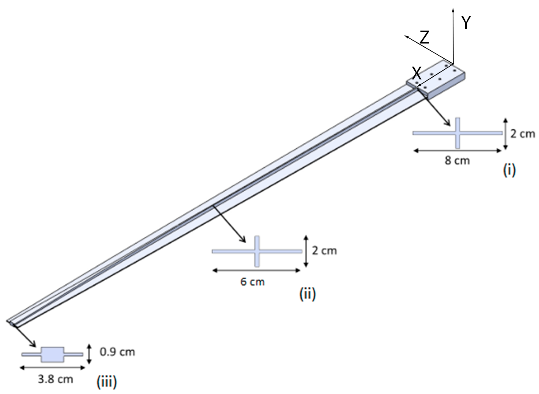
| Section | X [m] | Y [m] | Z [m] |
|---|---|---|---|
| Root | 0.125 | 0 | 0 |
| Mid-span | 0.875 | 0 | 0 |
| Tip | 1.45 | 0 | 0 |
| Specimen | Description | Mass [kg] |
|---|---|---|
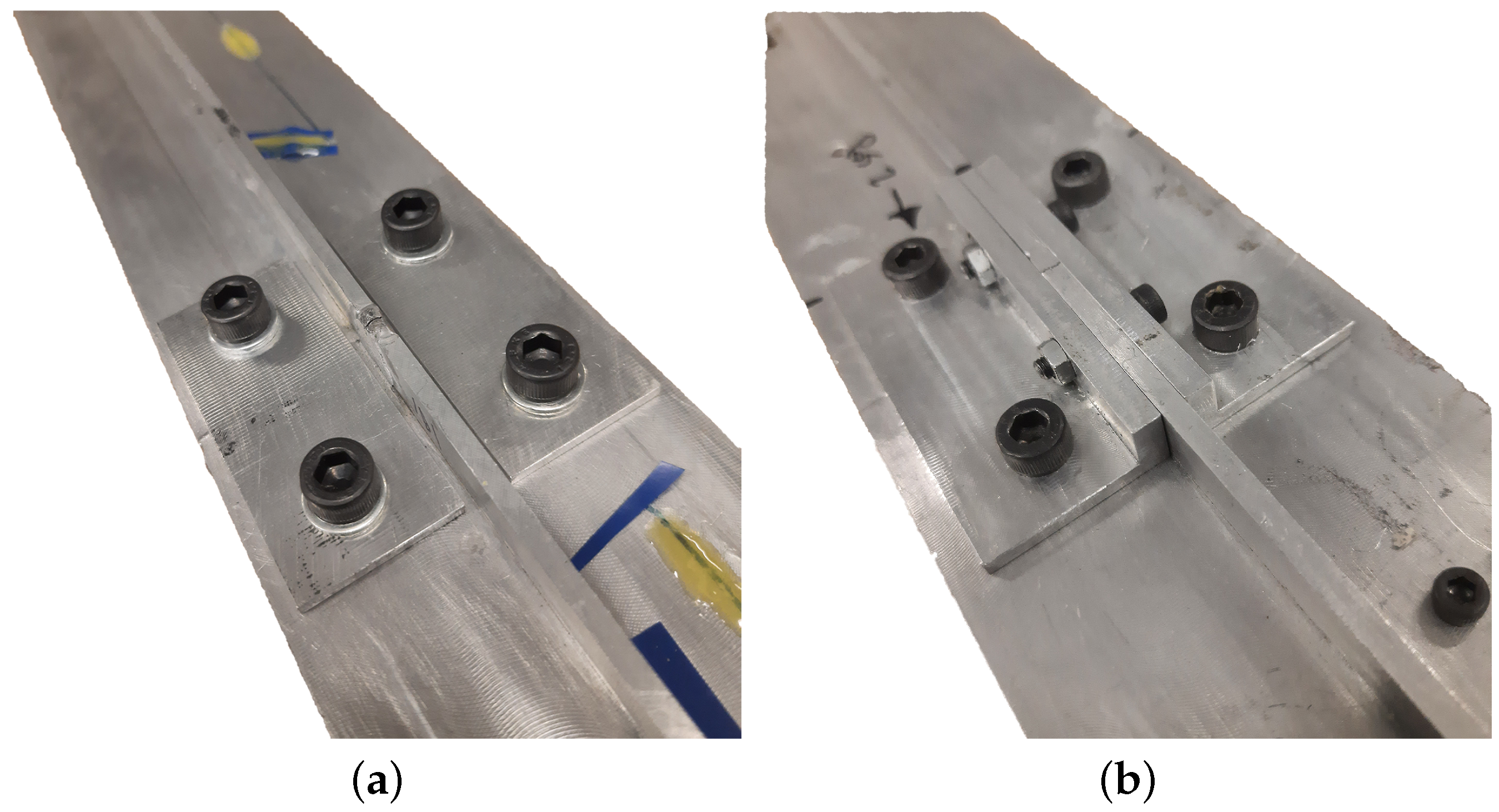
| Twin spar | The twin spar is a spar that was manufactured for ground testing only and it is recognisable from the main, or actual, spar for its bridge plate, as shown in Figure 4a. | 1.220 |
| Main spar | This is the spar used for the wind tunnel testing of XB-2 and its recognisable from the twin spar for its deformed shape and L profiled bridge plate, Figure 4b. | 1.225 |
| Section | X [m] | Y [m] | Z [m] |
|---|---|---|---|
| Tube inner end | 0.157 | −0.002 | 0.045 |
| First link | 0.170 | 0 | 0.045 |
| Second link | 0.430 | 0 | 0.045 |
| Third link | 0.690 | 0 | 0.045 |
| Tube outer end | 0.707 | −0.002 | 0.045 |
| Bending Mode | Theoretical | Numerical | GVT [3] |
|---|---|---|---|
| 1st | 5.166 | 5.183 | 5.27 |
| 2nd | 32.373 | 30.837 | 27.12 |
| 3rd | 90.646 | 106.060 | 83.39 |
| Specimen | Description | Mass [kg] |
|---|---|---|
| Twin spar | The twin spar is a spar that was manufactured for ground testing only, and it is recognisable from the main, or actual, spar for its bridge plate, as shown in Figure 4a. | 1.220 |
| Main spar | This is the spar used for the wind tunnel testing of XB-2 (Figure 4b). | 1.225 |
| Spar and tube | The spar and tube is the torque box of XB-2, which includes the main spar and the tube (Figure 5). | 1.362 |
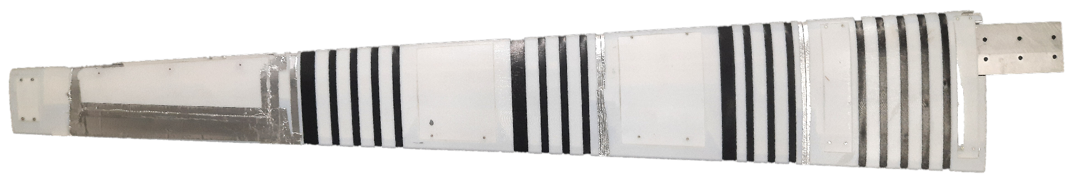
| Full wing | This is the XB-2 wing, comprising spar, tube and skin (Figure 2). | 3.024 |
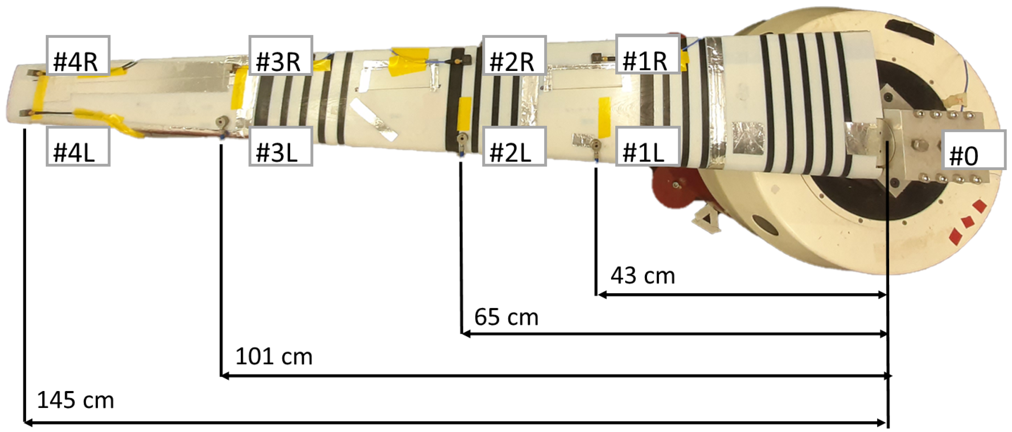
| ID # | Accelerometers Model | Sensitivity [mVg] | Mass [g] |
|---|---|---|---|
| 0 | PCB Piezotronics® model: 352C23 | 4.88 | 0.2 |
| 1R | PCB Piezotronics® model: 356A16 | 96.5 | 7.4 |
| 1L | Isotron® accelerometer model 7251A | 10.3 | 10.5 |
| 2R | PCB Piezotronics® model: 356A16 | 97.2 | 7.4 |
| 2L | Isotron® accelerometer model 7251A | 10.08 | 10.5 |
| 3R | PCB Piezotronics® model: 356A45 | 100.2 | 4.2 |
| 3L | Isotron® accelerometer model 7251A | 10.34 | 10.5 |
| 4R | Brüel & Kjær® accelerometer type 4507-002 | 94.12 | 4.8 |
| 4L | Brüel & Kjær® accelerometer type 4507-002 | 95.52 | 4.8 |
| Input | ||||||
|---|---|---|---|---|---|---|
| Bending Mode | Low | Medium | High | |||
| [Hz] | [-] | [Hz] | [-] | [Hz] | [-] | |
| 1st | 4.731 | 0.013 | 4.742 | 0.027 | 4.738 | 0.029 |
| 2nd | 24.732 | 0.010 | 25.021 | 0.021 | 25.087 | 0.016 |
| 3rd | 75.939 | 0.017 | 75.124 | 0.021 | 75.016 | 0.022 |
| Input | ||||||
|---|---|---|---|---|---|---|
| Bending Mode | Low | Medium | High | |||
| [Hz] | [-] | [Hz] | [-] | [Hz] | [-] | |
| 1st | 4.855 | 0.033 | 4.866 | 0.029 | 4.876 | 0.029 |
| 2nd | 26.966 | 0.010 | 27.050 | 0.016 | 27.057 | 0.014 |
| 3rd | 76.851 | 0.014 | 76.195 | 0.020 | 75.805 | 0.022 |
| Input | ||||||
|---|---|---|---|---|---|---|
| Bending Mode | Low | Medium | High | |||
| [Hz] | [-] | [Hz] | [-] | [Hz] | [-] | |
| 1st Bending | 5.252 | 0.022 | 5.151 | 0.030 | 5.163 | 0.036 |
| 2nd Bending | 25.933 | 0.014 | 25.958 | 0.011 | 25.941 | .010 |
| 3rd Coupled | 76.242 | 0.017 | 75.770 | 0.034 | 75.135 | 0.034 |
| Input | ||||||
|---|---|---|---|---|---|---|
| Bending Mode | Low | Medium | High | |||
| [Hz] | [-] | [Hz] | [-] | [Hz] | [-] | |
| 1st Bending | 3.187 | 0.024 | 3.164 | 0.018 | 3.139 | 0.018 |
| 2nd Coupled | 11.752 | 0.047 | 11.267 | 0.060 | 11.196 | 0.065 |
| 4th Coupled | 17.447 | 0.037 | 17.070 | 0.041 | 16.988 | 0.042 |
Publisher’s Note: MDPI stays neutral with regard to jurisdictional claims in published maps and institutional affiliations. |
© 2022 by the authors. Licensee MDPI, Basel, Switzerland. This article is an open access article distributed under the terms and conditions of the Creative Commons Attribution (CC BY) license (https://creativecommons.org/licenses/by/4.0/).
Share and Cite
Dessena, G.; Ignatyev, D.I.; Whidborne, J.F.; Pontillo, A.; Zanotti Fragonara, L. Ground Vibration Testing of a Flexible Wing: A Benchmark and Case Study. Aerospace 2022, 9, 438. https://doi.org/10.3390/aerospace9080438
Dessena G, Ignatyev DI, Whidborne JF, Pontillo A, Zanotti Fragonara L. Ground Vibration Testing of a Flexible Wing: A Benchmark and Case Study. Aerospace. 2022; 9(8):438. https://doi.org/10.3390/aerospace9080438
Chicago/Turabian StyleDessena, Gabriele, Dmitry I. Ignatyev, James F. Whidborne, Alessandro Pontillo, and Luca Zanotti Fragonara. 2022. "Ground Vibration Testing of a Flexible Wing: A Benchmark and Case Study" Aerospace 9, no. 8: 438. https://doi.org/10.3390/aerospace9080438