Using Reinforcement Learning to Improve Airspace Structuring in an Urban Environment

Abstract

Current predictions on future drone operations estimate that traffic density orders of magnitude will be higher than any observed in manned aviation. Such densities redirect the focus towards elements that can decrease conflict rate and severity, with special emphasis on airspace structures, an element that has been overlooked within distributed environments in the past. This work delves into the impacts of different airspace structures in multiple traffic scenarios, and how appropriate structures can increase the safety of future drone operations in urban airspace. First, reinforcement learning was used to define optimal heading range distributions with a layered airspace concept. Second, transition layers were reserved to facilitate the vertical deviation between cruising layers and conflict avoidance. The effects of traffic density, non-linear routes, and vertical deviation between layers were tested in an open-source airspace simulation platform. Results show that optimal structuring catered to the current traffic scenario improves airspace usage by correctly segmenting aircraft according to their flight routes. The number of conflicts and losses of minimum separation was reduced versus using a single, uniform airspace structure for all traffic scenarios, thus enabling higher airspace capacity.

1. Introduction

The European drones outlook study [1] estimates that as many as 400,000 drones will be operating in the airspace by 2050. The use of machine learning in tactical conflict detection and resolution (CD&R) is a tool that could potentially support advanced and scalable access to the airspace for a large number of drone (U-space) services. The present work aids this research by developing a reinforcement learning module that selects the optimal airspace structure for the current traffic, decreasing the conflict severity and rate for unmanned aviation operations in urban environments. A conflict is a predicted future loss of minimum separation (LoS). A loss of minimum separation (or intrusion) occurs when two aircraft are closer to each other than the minimum separation distance. The paramount objective of air traffic control (ATC) is to prevent intrusions.

Airspace structure plays a positive role in airspace capacity. Within centralized ATC, structuring consists of separating the airspace into different sectors. Each air traffic controller (ATCo) is responsible for one sector. The number of aircraft in each sector is limited to how many aircraft each ATCo can control simultaneously [2]. However, it is yet not clear how to optimally structure a distributed airspace. The Metropolis Project explored different types of airspace structures for manned flights in a dense urban area, using distributed separation assurance [3]. Results showed that a ‘layers’ concept, where the available airspace is segmented vertically, increases airspace capacity by reducing the number of conflicts and losses of minimum separation. This concept was further developed recently for unmanned aviation [4], where all directions within an urban infrastructure were divided per the available vertical layers. This research focused on a single, uniform structure and analyzed its effect. The present work builds upon the latter by exploring optimized structures catered to the expected traffic scenario.

Research related to road vehicles explored reinforcement learning (RL) to improve lane configuration [5,6]. Dynamic lane configurations reduced the average travel time in congested road networks when compared to a fixed, traditional lane-direction configuration [7]. Fixed configurations assume pre-known, static traffic patterns. However, in the real world, traffic may change considerably; one single configuration is not necessarily optimal for all traffic situations [8]. Urban air traffic has several similarities with road traffic that justify exploring machine learning techniques successfully applied in the latter [9,10]. First, unmanned aviation is set to follow road infrastructure [11]. Thus, the effects of the environment topology on traffic agglomeration are similar in both cases. Collisions are prevented by maintaining a minimum distance between vehicles, comparable to aviation. However, there are remarkable differences between drones and road vehicles. The latter can become stationary, but not all drones can hover [12]. Additionally, in aviation, minimum separation distances are typically larger. These challenges will be further examined in this work.

This study used the open-source, ATC simulation tool BlueSky [13] to simulate operations in an urban environment. Aircraft follow pre-planned routes around urban infrastructure (thus, preventing collisions with static obstacles). Conflicts between aircraft are resolved with conflict resolution (CR) with implicit coordination. This work resorted to CR model modified voltage potential (MVP) [14], which has proved effective in reducing losses of separation with minimal state deviation [15]. Normally, most conflict detection and resolution (CD&R) methods favor heading deviations as preferred by air traffic controllers. However, in an urban environment, such deviations could result in collisions with the surrounding infrastructure. We favor a speed and altitude-based conflict resolution approach, guaranteeing that the frontiers with the surrounding urban infrastructure are always respected. Finally, the deep deterministic policy gradient (DDPG) [16] model was used to determine optimal directions per layer within a layered airspace concept.

2. Related Work

ATM is a critical domain, with safety as the top priority, which explains the slow progress in the use of machine learning (ML) approaches in the ATM domain when compared to other research fields [17]. Here, we focus on the application of ML for airspace design. The body of work in this area is narrow; ML approaches are often limited to assessing the complexity in an airspace sector. Brito [18] used supervised learning to predict air traffic demand in airspace sectors, enhancing the predictability of airspace sector demand versus a baseline demand estimation model, which mimics the current practice. Li [19] employed an unsupervised learning approach for the airspace complexity evaluation; results showed that it outperformed state-of-the-art methods in terms of airspace complexity evaluation accuracy. Finally, Wieland [20] showed that ML approaches can help determine the importance of each complexity feature in predicting airspace capacity.

Regarding airspace structuring, existent ML methods are more directed at manned aviation, focusing on airspace sectors. Xue [21] approached dynamic vector resectorization with Voronoi diagrams and genetic algorithms. Results show that these are capable of determining the dominant traffic flow, which is one of the main concerns in sector design. Kulkarni [22] used dynamic programming to partition airspace based on the ATCos workload, showing that this could be a viable tool. Finally, Tang [23] proposed an agent-based model to dynamically partition the airspace, to accommodate the traffic growth while satisfying efficiency metrics. The trained models showed promising results both in balancing the ATCos workload and the average sector flight time.

To the best of the authors’ knowledge, this is the first work that approaches airspace structuring for unmanned aviation environments. The latter entails a very specific challenge: these types of operations entail a much higher number of heading deviations (i.e., turns during the flight route) than manned aviation, where aircraft employ (as much as possible) direct routes from the start to the endpoint. We employed an urban environment with the objective of ‘forcing’ turns to see whether the RL method could adapt to these changes. Nevertheless, the RL method herein employed could also be applied to layered airspace without turns and roads. In this case, the RL method should be used to define the heading ranges in each vertical layer.

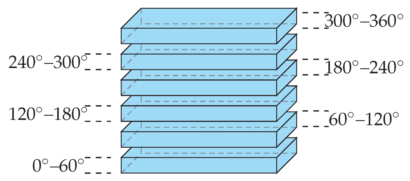
3. Layered Urban Airspace Design

The usage of drones in an urban environment entails several challenges. Separation with the urban infrastructure must be guaranteed at all times. Most of the current tactical CD&R methods are directed at manned aviation, aimed at detecting other flying traffic at cruise altitude. A model directed at dynamic obstacles cannot automatically be translated to defend against static obstacles. In most existing research on tactical conflict resolution, static obstacles are predominantly defined as (sparse) objects to fly around, as opposed to a multitude of objects that dominate the available space to operate [24]. This work considers that aircraft follow a pre-defined safe route around all static obstacles. Waypoints are set at the center of the roads, from which aircraft do not deviate.

Conflict resolution is not as efficient as it would be in non-constrained airspace, as aircraft cannot modify their headings to avoid conflicts. Near head-on conflicts are practically impossible to resolve without heading deviation. The focus must then be on conflict prevention. Airspace structures directly reduce conflict probability by decreasing the likelihood of aircraft meeting during their flights. The Metropolis Project has shown that a layered airspace structure considerably reduces the rate of conflicts [25]. Two effects contribute to this reduction. First, the total traffic density is segmented into groups of aircraft allocated at different altitude layers. Second, these groups are divided per aircraft heading, enforcing a degree of alignment between the aircraft, which decreases the likelihood of conflicts in each layer.

Previous research [4,26,27,28] investigated the layered concept in urban environments. However, only evenly distributed heading ranges per layer (as exemplified in Figure 1) have been researched. However, this is only optimal when the heading distribution of the traffic is uniformly distributed as well. In reality, this is often not the case. Flights may be performed predominantly in specific directions, following the topology of the bigger avenues in the urban environment. Aircraft may be expected to heavily move towards areas with higher population densities, or to a few specific storage points when employed for delivery purposes. Additionally, the directions of flight may change often as aircraft redirect at intersections to avoid collisions with static obstacles.

Aircraft will not be equally distributed over the available airspace when the structure of the airspace does not align with the current heading distribution. One layer will have a higher traffic density than the others when aircraft predominantly adopt a certain direction. In the worst-case scenario, the segmentation factor will be lost, canceling out the benefit of having a layered structure. Thus, the airspace structure should be set as a function of the current traffic scenario to prevent conflicts and reduce travel time. Moreover, given the fast-changing nature of the traffic, an automated control is preferable to guarantee fast response times and higher structure variability. In this work, we propose a reinforcement learning approach responsible for defining the heading range per traffic layer as a function of the expected traffic scenario. The objective is for this automated agent to focus on dividing aircraft per layer according to the real distribution, making full use of the available airspace.

4. Airspace Structure with Reinforcement Learning

4.1. Agent

We employed an RL agent whose objective was to set an optimized structure that catered to the expected traffic scenario. We assumed that the agent had full information on the future traffic density and trajectories. In a real-world application, this agent might be seen as a component responsible for defining the structure of the operational airspace.

4.2. Learning Algorithm

An RL model consists of an agent interacting with an environment E in discrete timesteps. At each timestep, the agent receives the current state s of the environment and performs an action a in accordance with which it receives a reward $r_t$. An agent’s behavior is defined by a policy, $\pi$, which maps states to actions. The goal is to learn a policy that maximizes the reward. Many RL algorithms have been researched in terms of defining the expected reward following action a. In this work, we used the deep deterministic policy gradient (DDPG), defined in [16].

Policy gradient algorithms first evaluate the policy and then follow the policy gradient to maximize the performance. DDPG is a deterministic actor–critic policy gradient algorithm, designed to handle continuous and high-dimensional state and action spaces. It has proven to outperform other RL algorithms in environments with stable dynamics [29]. Additionally, DDPG has been successfully implemented in the aviation environment [30,31,32], proving that it can adapt to aircraft dynamics. However, DDPG can become unstable, being particularly sensitive to reward scale settings [33,34]. As a result, rewards must be carefully defined.

DDPG is an instance of the actor–critic model. The deterministic actor receives a state from the environment and outputs an action. The critic maps each state–action pair, informing the actor how to adjust towards outputting the best actions. Furthermore, the DDPG model employs target networks and a replay buffer. The target networks are mostly useful to stabilize function approximation when learning for the critic and actor networks. The replay buffer stores multiple past experiences, from which mini-batch samples are used to update the actor and critic. The pseudo-code for DDPG is displayed in Algorithm 1. Additionally, exploration noise was added to promote exploration of the environment; an Ornstein–Uhlenbeck process [35] was used in parallel with the authors of the DDPG model.

Algorithm 1 Deep deterministic policy gradient.

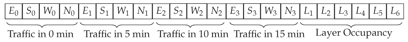
Initialize critic $Q\left(s\right|a^{\mu })$ and actor $\mu \left(s\right|{\theta }^{\mu })$ networks Initialize replay buffer R for all episodes do    Initialize action exploration    while episode not ended do      Select action $a_t$ according to the current state $s_t$ from the environment and the current actor network      Perform action $a_t$ in the environment and receive a reward $r_t$ and new state $s_{t+1}$      Store transition $(s_t,a_t,r_t,s_{t+1})$ in the replay buffer R      Sample a random mini-batch of N transitions from R      Update critic by minimizing the loss      Update the actor policy using the sample policy gradient      Update the target networks    end while    Reset the environment end for

Table 1. Hyperparameters of the employed RL method used in this work.

Parameter	Value
TAU	0.001
Learning rate actor (LRA)	0.0001
Learning rate critic (LRC)	0.001
EPSILON	0.1
GAMMA	0.99
Buffer size	1 M
Minibatch size	256
# Hidden layer-neural networks	2
# Neurons	120 in each layer
Activation functions	Rectified linear unit (ReLU) in the hidden layers
	Softmax in the last layer

presents the hyperparameters employed in this work. We resorted to two hidden layer-neural networks with 120 neurons in each layer. Both layers used the rectified linear unit (ReLU) activation function.

4.3. State

The state input into the RL model must contain the necessary data for the RL agent to successfully determine an optimal heading division per traffic layer. We consider that such a decision requires information on the traffic demand, flight routes, and their evolution over time. However, representing correct traffic flow evolution is non-trivial and can assume various shapes. Moreover, with RL, a simplified representation of the environment is often needed to optimize the training of the neural network. Representing the complete flight routes for all aircraft would greatly increase the size of the state formulation and with it the number of possible states and state–action combinations. As the size of the problem’s solution space grows exponentially with the number of states, it may reach a point where the training time becomes unrealistic.

Therefore, we assumed a state array with a fixed dimension representing a simplified version of the environment. Based on the pre-defined routes, ‘snapshots’ were made of certain points in time. Each point in time was defined by four variables, with each variable representing the number of aircraft in each of the four possible directions: east, south, west, and north. Figure 2 represents the complete state array. A total of four ‘snapshops’ were taken, each one further in time by five minutes. For example, $E_1$ represents the number of aircraft traveling in the east direction at minute five past the start of the traffic scenario. Naturally, having more ‘snapshops’ provides more information regarding the environment but at the cost of adding more complexity to the model.

Additionally, for simplification, a fixed number of vertical layers was assumed. Six traffic layers were defined. The six final elements of the state array ($L_1$ to $L_6$) were used to indicate the current number of aircraft in each traffic layer. It was considered that the structure was set before the aircraft initiated their flights. Thus, the airspace was empty at the beginning of each episode, and the six final positions equaled 0 in the initial state. However, at the end of the episode, as the RL model was informed of the next state, this information became relevant. Ideally, the RL agent should opt for a structure that homogeneously divides aircraft across the available airspace (segmentation effect). Additionally, this state formulation could potentially be used in a situation where the traffic volume at the beginning of the episode is not zero as it is capable of transmitting such information.

4.4. Action

The RL agent determines the action to be performed for the current state. The incoming state values are transformed through each layer of the neural network, in accordance with the neuron weights and the activation function in each layer. The activation function takes in the output values from the previous layer and converts them into a form that can be taken as the input for the next layer. The output of the final layer must be turned into values that can be used to define the heading range in each traffic layer. A softmax activation function was employed in the last layer; the output values were used to define which direction was allowed at each traffic layer. Since there was a maximum of four possible directions, and a total number of six layers, the dimension of the action array was set to twenty-four (four directions × six layers). Figure 3 shows how the necessary information was extracted from the action array. For example, the first four positions of the array corresponded to the four directions possible in the first layer; the direction with the highest integer value was picked.

Thus there are two main components upon which the RL agent decides:

• The number of layers for each direction: the RL agent may decide to select more layers for a direction adopted by the majority of aircraft. However, an important safeguard was implemented upon the airspace structure output by the RL agent. To make sure that all directions were allowed in the airspace, a final check was applied to the structure. If all possible directions were not yet allowed, the last layer was overwritten to allow for the missing directions. Note that it may occur that more than one flight direction is allowed in this layer.
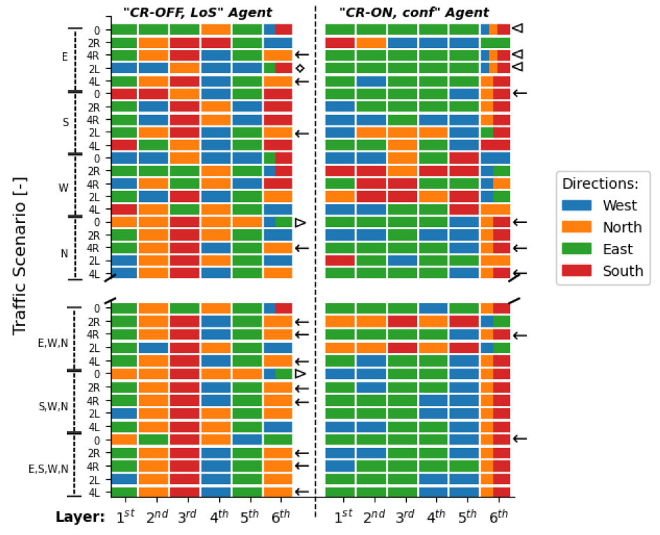
• The order of the layers: the RL agent decides which directions are in adjacent layers. For a fixed structure, it is good practice to allow the left or right turning by just climbing or descending one layer. However, on purpose, the agent is free to choose the order of directions. It will be evaluated whether the structure output by the RL agent includes an understanding of perpendicular directions.

4.5. Reward

The RL model should prioritize safety, with the paramount factor being the likelihood of conflicts or LoSs. However, it is unclear, at this state, which element will result in a more optimal convergence—the total number of conflicts, or the total number of losses of minimum separation. As a result, the following reward formulations will be tested and compared:

• The RL model receives a −1 for each conflict.
• The RL model receives a −1 for each loss of minimum separation.

A loss of separation is detected when two aircraft are closer to each other than the minimum separation distance. A conflict is a predicted future loss of minimum separation. More details on the state-based conflict detection used in this work are given in Section 5.6.

Note that a considerable limitation of this reward formulation is the fact that it does not take into consideration efficiency, more specifically, (1) extra energy consumption resulting from drones traversing between layers far away, and (2) extra energy consumption due to the vertical conflict avoidance maneuvers. Urban air mobility vehicles are limited (energy-wise). Thus, these maneuvers can hinder the paths and travel times of these vehicles. Nevertheless, this work is the first approach intended to study whether RL methods can successfully set an airspace structure adapted to the traffic scenario; thus, we opted for a simple reward formulation focusing only on safety. Notwithstanding, it may be considered that safety has an indirect positive effect on efficiency: decreasing both the total number of conflicts or LoSs directly reduces the number of vertical conflict avoidance maneuvers. Future work should consider efficiency elements as well. Nevertheless, weights of safety and efficiency should be carefully considered. Safety should not be jeopardized in favor of faster or longer flight routes.

5. Experiment: Safety-Optimized Airspace Structures

The following subsections define the properties of the performed experiment. The latter aims at using RL to define the heading range at each vertical traffic layer within layered urban airspace. Note that the experiment involves a training and a testing phase. First, the RL model was trained continuously with a set of traffic scenarios. Second, it was tested with unknown traffic scenarios. Performances with these new scenarios are directly compared to a baseline that employed evenly distributed heading ranges per layer.

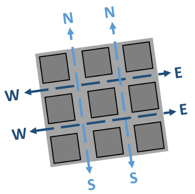
5.1. Simulated Environment

We first define the simulation area. This is an urban setting built using the Open Street Map networks (OSMnx) python library [36], an open-source tool for street network analysis. We used an excerpt from the San Francisco Area, representing an orthogonal street layout with an area of $1.708$ NM2, as depicted in Figure 4. The OSMnx library returned a set of nodes from which a network of roads could be defined.

In this area, roads and intersections were defined by vertices and nodes, respectively. Two adjacent nodes represent the edges of a road. Aircraft can only travel from one node to another when these are connected. With the intention of reducing complexity, each node was considered to have (upmost) four connecting roads, as shown in Figure 5. Only existing roads were considered. Additionally, we assumed that each road was unidirectional, with only one lane. We did not make any assumption regarding the width of the road, which would have been needed if more directions were considered.

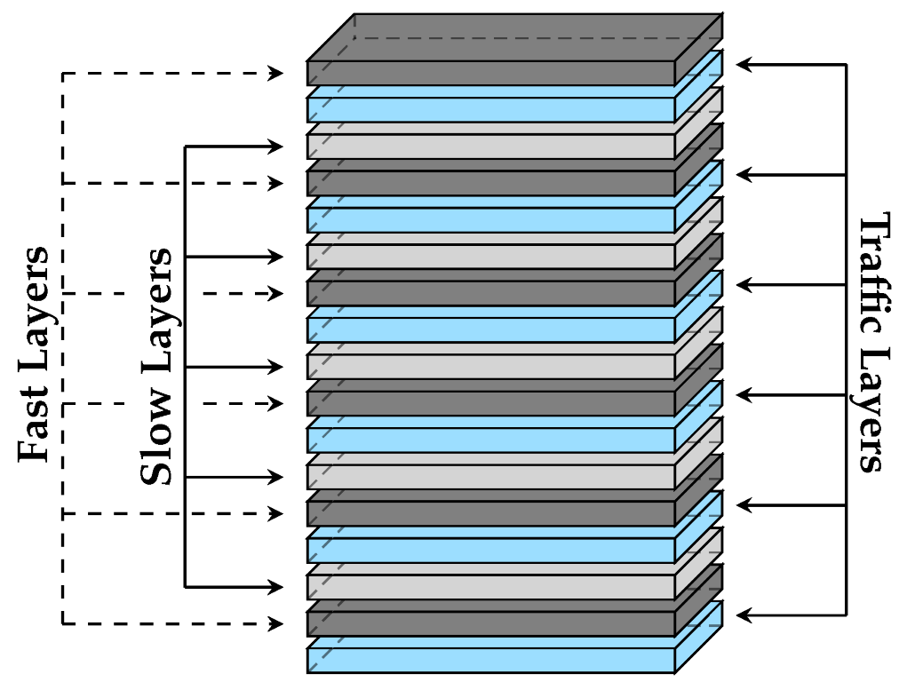
5.2. Transition Layers

In conventional aviation, temporary altitude layers are often used as a level-off at an intermediate flight level along a climb or descent to avoid conflicts [37]. In our urban airspace, we applied the same concept: we included (low-speed) transition layers in the airspace to be used only by aircraft that were transitioning between traffic layers. Aircraft performed the heading turns in these transition layers, preventing conflicts resulting from heterogeneous speed situations when an aircraft decelerated just before a turn. Transition layers were expected to be (almost) depleted of aircraft at any point in time, reducing the likelihood of aircraft meeting in conflict. Moreover, we considered that aircraft flew along the middle of the road. Since we also made no assumptions about the width of a street, aircraft were also not allowed to use heading changes for conflict resolution. This means that aircraft could only resort to speed and altitude changes to avoid conflicts. However, a vertical space needs to be reserved for vertical conflict resolution, preventing aircraft from entering adjacent traffic layers. Thus, additional vertical layers were allocated for this purpose. Figure 6 depicts the different layers used in the experimental scenario.

Three different layer types were considered, each dedicated to different actions:

• Six traffic layers (in blue): the main layers used by cruising traffic.
• Six slow transition layers (in light grey) were used for transitioning between traffic layers. This is a necessary mid-step prior to the aircraft entering different traffic layers. First, the aircraft exit the current traffic layer without modifying their speed, in order to not create conflict with other cruising aircraft, and they move toward the slow layer. Here, the aircraft decrease their speed to reach the speed required to comply with the turn radius. After turning, the aircraft start accelerating toward the desired cruising speed/moving to the destination traffic layer.
• Six fast transition layers (in dark grey) were used to perform vertical conflict avoidance when necessary. The overtaking aircraft resolve the conflict by moving into the fast layer; aircraft being overtaken have the right of way. Once the conflict is resolved, the aircraft move back into the traffic layer to guarantee that the fast layers are (mostly) depleted of other traffic when the aircraft need to perform vertical resolution.

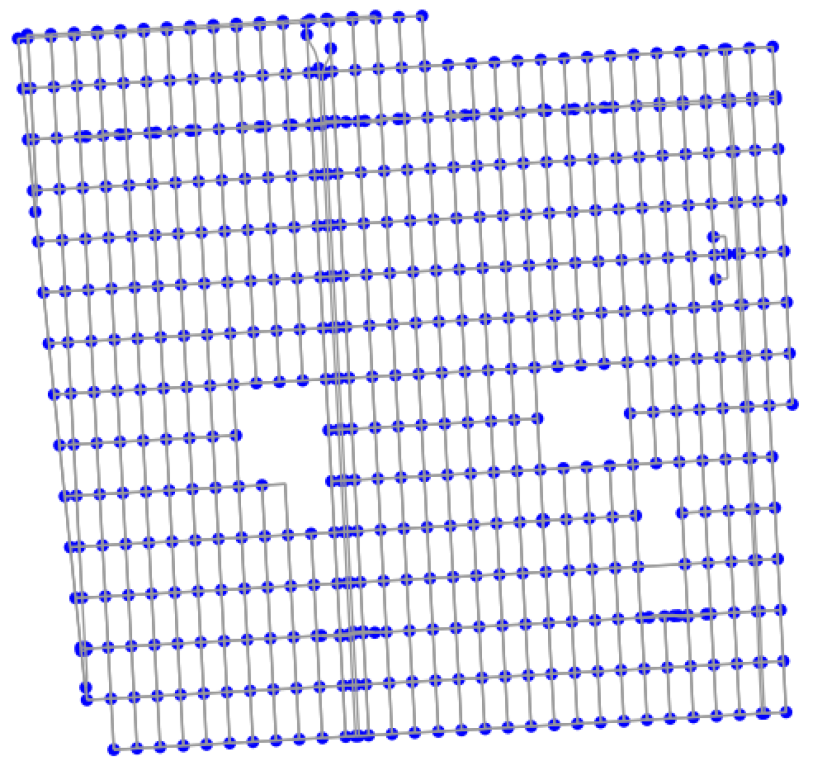
All layers were set with a height of 15 ft. There was a margin of 5 ft between the layers to prevent false conflicts.

5.3. Flight Routes

Aircraft spawn locations (origins) were placed in alternating orders on the edge of the simulation area, with a minimum spacing equal to the minimum separation distance, to avoid conflicts between spawn aircraft and aircraft arriving at their destinations. Multiple traffic layers were used; aircraft were spawned at the altitude of a layer that allowed for the initial heading. Aircraft climbed almost vertically. Finally, an aircraft was deleted from the simulation once it left the simulation area. To prevent aircraft from being removed incorrectly when traveling through an edge road, aircraft were set to move out of the map once they finished their route and were removed once they moved away from an edge node.

Each aircraft has several waypoints it must pass through. These are always nodes from the map and are calculated based on the defined initial direction, number, and direction of turns, as displayed in

Table 2. Flight routes are defined as per the initial direction and the number of turns. The aircraft initial distribution defines, for each scenario, the percentage of flights starting in each initial direction. A total of 15 scenarios with different initial distributions were used. Each scenario was performed five times, with a different number and direction of turns.

Traffic Scenario:		#1	#2	#3	#4	#5	#6	#7	#8	#9	#10	#11	#12	#13	#14	#15
% A/C Initial Hdg Distribution	East (E):	100	0	0	0	50	50	50	0	0	0	33	33	33	0	25
	South (S):	0	100	0	0	50	0	0	50	50	0	33	33	0	33	25
	West (W):	0	0	100	0	0	50	0	50	0	50	33	0	33	33	25
	North (N):	0	0	0	100	0	0	50	0	50	50	0	33	33	33	25
Flight Path With Turns:		All traffic scenarios are repeated with:							•No Turns (0) •2 Turns to the Right (2R) •4 Turns to the Right (4R) •2 Turns to the Left (2L) •4 Turns to the Left (4L)

. There were a total of 75 traffic scenarios (15 initial heading distribution × 5 turns) per traffic density. During the creation of the simulation scenarios, the total flight time of the already created aircraft was accounted for so that the desired instantaneous traffic densities were respected. All aircraft started at the corresponding end of the map, allowing for a linear route towards their initial directions (e.g., an aircraft with an initial direction of the east will start at the west end of the map). If there are no turns, the aircraft will travel in their initial directions throughout the complete route. A turn to the right from an aircraft with the initial direction east indicates that the aircraft will turn south during its route. A turn to the left would result in this aircraft turning north.

During the training of the RL model, one set of 75 traffic scenarios with medium traffic density was used. During testing, three different sets of each traffic density (low, medium, and high traffic density) were run. Thus, testing was conducted for three different trajectories for each combination of initial direction and the number of turns. This variability of traffic scenarios is aimed at testing the performance of the RL model in multiple situations. Using different heading distributions tests the capacity of the RL model to successfully segment different traffic scenarios over the available airspace. Using a different number of turns tests the ability of the model to protect against successive changes in the heading distribution.

5.4. Apparatus and Aircraft Model

The open-air traffic simulator BlueSky [13] was used to test the efficiency of dynamic airspace structuring. The performance characteristics of the DJI Mavic Pro were used to simulate all vehicles. Here, speed and mass were retrieved from the manufacturer’s data, and common conservative values were assumed for the turn rate (max: $15{}^{\circ }/\mathrm{s}$), acceleration, and breaking ($1.0 \mathrm{k}\mathrm{t}\mathrm{s}/\mathrm{s}$).

5.5. Minimum Separation

The appropriate minimum safe separation distance depends on the operational environment and type of aircraft involved. For unmanned aviation, there are no established separation distance standards yet. We opted for 50 m for horizontal separation, as commonly used in research [38]. For vertical separation, 15 ft was assumed, based on the dimension of the vertical layers.

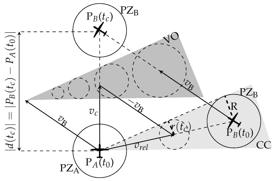
5.6. Conflict Detection

This study employed state-based conflict detection, which assumes the linear propagation of the current state of all aircraft involved. Thus, the time to the closest point of approach (CPA), in seconds, is calculated as:

$$t_{CPA}=-\frac{{\overrightarrow{d}}_{rel}·{\overrightarrow{v}}_{rel}}{{\overrightarrow{v}}_{rel}},$$

(1)

where ${\overrightarrow{d}}_{rel}$ is the Cartesian distance vector between the involved aircraft (in meters) and ${\overrightarrow{v}}_{rel}$ is the vector difference between the velocity vectors of the involved aircraft (in meters per second). The distance between aircraft at CPA (in meters) is calculated as:

$$d_{CPA}=\sqrt{{\overrightarrow{d}}_{rel}^2-{t_{CPA}}^2·{{\overrightarrow{v}}_{rel}}^2}.$$

(2)

When the separation distance is calculated to be smaller than the specified minimal horizontal spacing, a time interval can be calculated in which separation will be lost if no action is taken:

$$t_{in},t_{out}=t_{CPA}\pm \frac{\sqrt{{R_{PZ}}^2-{d_{CPA}}^2}}{{\overrightarrow{v}}_{rel}}.$$

(3)

These equations will be used to detect conflicts, which are said to occur when $d_{CPA}<R_{PZ}$, and $t_{in}\le t_{lookahead}$, where $R_{PZ}$ is the radius of the protected zone or the minimum horizontal separation and $t_{lookahead}$ is the specified look-ahead time. A look-ahead time of 30 s was used for conflict detection and resolution.

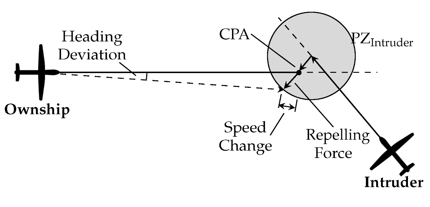
5.7. Conflict Resolution

To guarantee safety in between static obstacles (e.g., buildings, trees), movement within the horizontal plane was severely limited. For conflict resolution, we look at the remaining degrees of freedom, namely speed and altitude variations. Within an urban environment, we may consider two main conflict geometries: (1) conflicts with aircraft traveling along the same road; (2) conflicts at intersections. Within the first case, aircraft fly in the same direction; intruders are positioned directly in front or behind the ownship. These conflicts can be treated as pairwise conflicts, with a simple resolution, where each aircraft respects a minimum distance to the aircraft in front. The second type of conflict is more complicated. Crossing traffic flows, or merging aircraft, leads to multi-aircraft conflicts for which simple rules no longer suffice. For these conflicts, we resort to the velocity obstacle theory [39,40], which translates the two-dimensional problem of crossing flows into speed constraints, identifying which velocities result in conflicts.

Figure 7 exemplifies the construction of a velocity obstacle (VO). Ownship (A) is in conflict with an intruder (B). A collision cone (CC) can be defined as the triangular area between the lines tangential to the intruder’s protected zone (PZ). A and B are in conflict when the relative velocity between these two aircraft is inside the CC. A VO is defined as a collision cone translated by the intruder’s velocity; thus, expressing the separation constraints to the absolute velocity space of the ownship. This VO represents the set of ownship velocities that lead to a loss of separation with the intruder. R represents the radius of the PZ. $P_A\left(t_0\right)$ and $P_B\left(t_0\right)$ denote the initial positions of the ownship and the intruder, respectively. $P_B\left(t_c\right)$ identifies the intruder’s position at the moment of collision. Each intruder in the vicinity of an ownship results in a separate VO.

The geometric resolution of the MVP model, as defined by Hoekstra [14,42], is displayed in Figure 8. When a conflict is detected, MVP uses the predicted future positions of both ownship and intruder at the closest point of approach (CPA). These calculated positions ‘repel’ each other, and this ‘repelling force’ is converted to a displacement of the predicted position at CPA. The avoidance vector is calculated as the vector starting at the future position of the ownship and ending at the edge of the intruder’s protected zone, in the direction of the minimum distance vector. Thus, this displacement is the shortest way out of the intruder’s protected zone. Dividing the avoidance vector by the time left to CPA yields a new speed, which can be added to the ownship’s current speed vector, resulting in a new advised speed vector. From the latter, a new advised heading and speed can be retrieved. The same principle is used in the vertical situation, resulting in an advised vertical speed. In a multi-conflict situation, the final avoidance vector is determined by summing the repulsive forces with all intruders. As it is assumed that both aircraft in a conflict will take (opposite) measures to evade the other, MVP is implicitly coordinated.

5.8. Independent Variables

During training, reward formulation and conflict resolution were introduced as independent variables to observe how each influenced the training of the RL agent. During testing, different traffic densities were introduced to analyze how the RL model performed at traffic densities it was not trained in. Additionally, airspace structure outputs by the RL model were compared with a commonly used fixed, uniform airspace structure. More details are given below.

5.8.1. Reward Formulation

Two different reward formulations were tested and compared in terms of training efficiency: (1) −1 per each conflict; (2) −1 per each LoS.

5.8.2. Conflict Resolution

The effect of conflict resolution on the safety results was tested by directly comparing the efficacy of an RL agent trained in an environment without conflict resolution (CR-OFF), with another RL agent trained in an environment where MVP was used to generate conflict resolution maneuvers through speed and altitude variation (CR-ON).

5.8.3. Traffic Density

Traffic density varied from low to high as per

Table 3. Traffic volume used in the experimental simulations. The number of spawned aircraft correspond to 20 min of simulation time; the range results from different flight paths as the necessary time to traverse the environment is dependent on the initial direction(s) and the number of turns.

	Low	Medium	High
Traffic density [$ac/$10,000 NM ${}^2$]	292,740	585,408	878,112
Number of instantaneous aircraft [-]	50	100	150
Number of spawned aircraft [-]	80–397	159–794	236–1189

. The instantaneous aircraft value defined the number of aircraft expected at any given moment during the measurement period. At high densities, vehicles spent more than 10% of their flight times avoiding conflicts [43]. The RL agent responsible for setting the airspace structure was trained at a medium traffic density and was then tested with low, medium, and high traffic densities. In this way, it was possible to assess the efficiency of an agent performing in a traffic density different from that in which it was trained.

5.8.4. Airspace Structure

The airspace-structured output by the RL agent must be compared to a baseline-fixed structure ([W,N,E,S,W,N]), to verify that there is a significant improvement in having dynamic structuring catered to each traffic scenario versus one pre-defined structure. The latter is the structure defined in

Table 4. Quadrant rules for the baseline airspace structure used for comparison.

1st Layer (W)	2nd Layer (N)	3rd Layer (E)	4th Layer (S)	5th Layer (W)	6th Layer (N)
Altitude

, which obtained good results in previous research [44]. This baseline structure adopted one direction per vertical layer. In addition, it was possible to cross into a perpendicular road by climbing or descending to the next layer. The latter is the main benefit of this structure as it reduces the number of necessary vertical deviations.

5.9. Dependent Variables

Three different categories of measures were used to evaluate the effects of the different operating rules set in the simulation environment: safety, stability, and efficiency.

5.9.1. Safety Analysis

Safety was defined in terms of the number and duration of conflicts and losses of separation, where fewer conflicts and losses of separation are considered safer. Additionally, losses of separation are distinguished based on their severity according to how close the aircraft are to each other:

$$Lo{S}_{sev}=\frac{R-d_{CPA}}{R}.$$

(4)

A low separation severity is preferred.

5.9.2. Stability Analysis

Stability refers to the tendency for tactical conflict avoidance maneuvers to create secondary conflicts. In the literature, this effect has been measured using the domino effect parameter (DEP) [45]:

$$DEP=\frac{n_{cfl}^{ON}-n_{cfl}^{OFF}}{n_{cfl}^{OFF}},$$

(5)

where $n_{cfl}^{ON}$ and $n_{cfl}^{OFF}$ represent the number of conflicts with CD&R ON and OFF, respectively. A higher DEP value indicates a more destabilizing method, which creates more conflict chain reactions.

5.9.3. Efficiency Analysis

Efficiency is evaluated in terms of the distance traveled and the duration of the flight. There is a preference for methods that do not considerably increase the path traveled and/or the duration of the flight.

6. Experiment: Hypotheses

6.1. Simulated Traffic Scenarios

A set of 75 different scenarios was simulated for each traffic density (low, medium, and high traffic densities). During training, only the medium traffic density was employed; during testing, all three different traffic densities were employed. Within the different scenarios, different initial directions and the number of turns throughout the flight routes were set. This was an attempt at introducing a varying number of aircraft per direction and a different number of vertical deviations. Given that the traffic density was constant throughout each scenario, it was hypothesized that a smaller number of different initial traffic directions would lead to a higher number of conflicts and LoSs, due to the fact that all aircraft would be traveling in the same vertical layers, on the same ‘roads’. When more initial directions are in place, existing traffic is distributed among the airspace to a greater extent, reducing the probability of aircraft meeting in conflict. Additionally, it was hypothesized that a higher number of turns would be harder to optimize, as turns are not explicitly represented in the state formulation.

Nevertheless, looking only at the number of initial directions and turns is not enough to immediately identify the total number of conflicts and LoSs at the end of the simulation. Safety is also dependent on the trajectories taken and the topology of the environment. The latter may make some directions more prone to conflicts than others; the position of static obstacles may lead to certain locations turning into conflict ‘hotspots’. The latter will be analyzed with the experimental results.

6.2. Dynamic Airspace Structuring

It was hypothesized that having a dynamic airspace structure that catered to the expected traffic scenario would result in fewer conflicts and losses of minimum separation compared to having one fixed structure, which is not optimal for all different traffic cases. For an unbiased comparison, we must employ a fixed structure expected to perform reasonably well in a large range of different traffic scenarios. The structure (W, N, E, S, W, N) was chosen; the latter has been proven to be successful in previous research [44]. Naturally, it could even be that there are specific traffic scenarios for which this baseline structure is the most efficient and it may outperform the structure output by the RL model. This is relevant for comparison, to evaluate which structuring characteristics lead to an increase in safety.

6.3. Training of the Reinforcement Learning Model

It was hypothesized that employing conflict resolution during training of the RL model is optimal, as it is a better representation of the testing environment, where aircraft attempt to avoid each other. Additionally, having CR during training would allow optimization to focus on the conflicts that a geometric conflict resolution algorithm cannot resolve, instead of focusing on conflicts with small severity. The latter may be the majority but are easily resolved through conflict resolution. However, without conflict resolution, the RL agent can focus on conflict prevention; having fewer conflicts may result in fewer multi-conflicts situations.

Furthermore, the main objective of the RL agent is to reduce the LoS number, since this is the paramount value considered for safety. However, LoSs are sparse compared to conflicts, which may limit the optimal convergence of the RL model. The LoS number may not be sufficient for the RL to gather enough information for a proper understanding of the environment. Looking at conflicts results in more information for the RL agent, as these occur in higher numbers. Thus, the latter was hypothesized to warrant more optimal training. It is assumed that, although the total number of conflicts is not directly proportional to the number of LoSs [15], fewer conflicts lead to fewer LoSs.

Finally, testing of the RL agent included similar and different traffic densities to the training conditions. The agent was expected to perform better in the traffic density in which it was trained. However, applying the agent to different densities allowed one to assess how the efficiency of airspace structures varied with the traffic density. It was hypothesized that the agent may be the least effective at densities higher than the one it was trained in, as the complexity of the emergent behavior, and of the consequent solution, increased proportionally to the density.

7. Experiment: Results

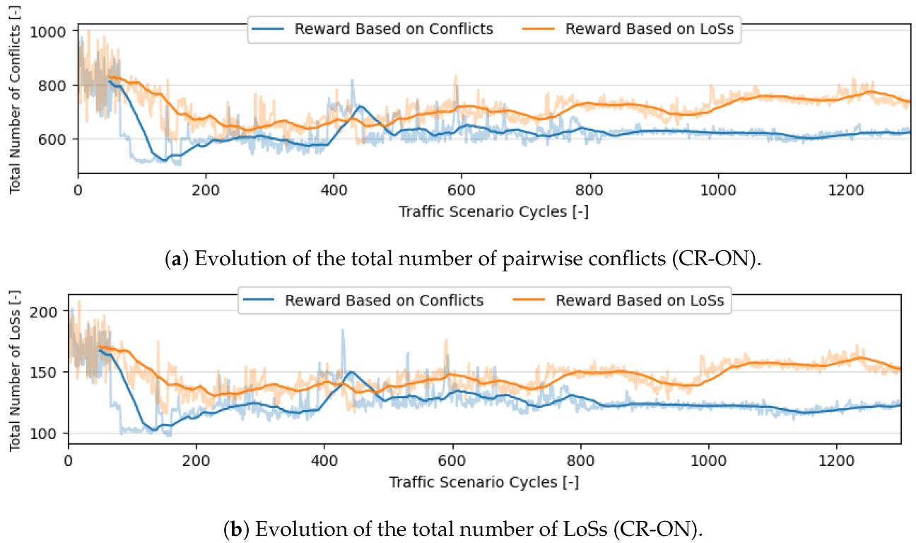
7.1. Training of the RL Agent for Safety-Optimized Airspace Structuring

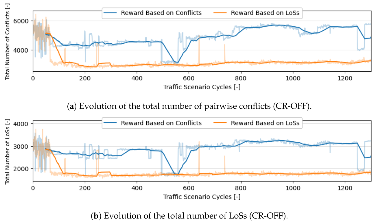
The RL agent responsible for setting the airspace structure was trained at a medium traffic density; 75 different traffic scenarios were tested repeatedly. These varied in the number of turns and initial direction(s), as previously described in Section 5.3. Each scenario execution corresponded to one episode, which, during the training phase, ran for 20 min. In total, 100,000 episodes were run. Thus, the set of (different) 75 episodes was repeated roughly 1330 times. Four (2 × 2) different RL agents were trained and compared directly to confirm the hypotheses set in Section 6.3; two agents were trained in an environment with CR (CR-ON), and two others without CR (CR-OFF). The two agents in each environment will be used to compare the efficiency of training based on LoSs and conflicts.

Safety Analysis

Figure 9 displays the evolution of the total number of pairwise conflicts and LoSs during training without CR. Each point represents the average conflicts or LoSs for 75 traffic scenario cycles. The shaded and solid lines represent all values and the moving average over the previous 50 values, respectively. For reference, the high variability at the beginning of the training was due to the impact of exploration noise. This noise was intentionally set stronger at the initial cycles to promote exploration. Its impact was reduced throughout training. We can see that although the number of conflicts and LoSs were strongly correlated, a LoS-based reward resulted in convergence to an optimal value whereas training based on conflicts did not. The former converged to a minimum number of conflicts and LoSs after approximately 200 cycles of the 75 training traffic scenarios ($200\times 75=15k$ episodes in total). Focusing on reducing the number of LoSs also reduced the number of conflicts. In comparison, training based on conflicts did not lead to finding an optimal value during a run of 100,000 episodes. There was no clear trend of decrement in conflicts throughout training. One possible reason is that the large magnitude of the total number of conflicts may have had a negative effect on performance. It could be that decreasing the reward per conflict, or normalizing the reward value, as is often done in practice to boost performance, could reduce the training time. However, such an investigation was deemed not relevant given the better success with a LoS-based reward.

Figure 10 shows the evolution of the total number of conflicts and LoSs during training with CR. The differences here are not as great as with the previous RL models trained without CR. However, contrary to the latter, the agent optimized based on the number of conflicts achieved fewer conflicts and LoSs. We consider this to be a direct consequence of the number of LoS occurrences in the environment. As hypothesized, in an environment with fewer LoSs, the number of conflicts is a better reward formulation, as its higher value provides more information to the RL agent. However, without conflict resolution, the number of LoSs and conflicts is higher. Thus, the LoS provides enough information and, being the paramount safety value, should be used.

The most effective RL agents, ‘CR-OFF, LoS’—the agent trained based on LoS in an environment without CR, and ‘CR-ON, conf’—the agent trained based on conflicts in an environment with CR, must now be directly compared within the same conditions. Figure 11 shows an example of the airspace structures produced by the two agents. Each row corresponds to one traffic scenario. For example, the first row identifies the traffic scenario where all aircraft initiated their flights directed east, and no turns were performed during the flight. The last row identifies the traffic scenario where aircraft initiated their flights directed east, south, west, or north (with equal distribution); each aircraft performed four turns to the left during their flights. The structure outputs by the ‘CR-OFF, LoS’ and ‘CR-ON, conf’ agents are displayed in the left and right columns, respectively.

In Figure 11, symbol (←) identifies the most employed airspace structure for each RL agent. Agent ‘CR-OFF, LoS’ used 28 different structures, with structure E,N,S,W,E,N being used in 29 of the traffic scenarios. This structure is employed more often when aircraft are more dispersed throughout the environment, i.e., when more different initial directions are employed. As expected, the more uniform the traffic scenario is, the more the RL agent tends to pick a structure where all directions have similar priority. In comparison, the ‘CR-ON, conf’ agent used 29 different structures, with structure E,E,E,E,W,(N,S) employed on 10 of the training traffic scenarios. This selection shows a different structure approach than the ‘CR-OFF, LoS’ agent. The latter opted for a uniform structure that performed relatively well for most traffic scenarios; the ‘CR-ON, conf’ agent preferred a structure that heavily focused on two directions—east and west—as per Figure 11. This is considered to be a direct result of applying the conflict resolution. CR resolves a lot of the conflicts that the ‘CR-OFF, LoS’ agent prevents with a structure that promotes even segmentation of aircraft throughout the airspace. Thus, the ‘CR-ON, conf’ agent focuses on conflict ‘hotspots’ at which CR is ineffective. Given that the most used structures strongly prioritize the west and east directions, this indicates that the topology of the environment leads to most of the ‘hotspots’ occurring when aircraft travel in the directions west–east and vice versa.

The efficacy of the segmentation performed by the RL agent is more clearly evaluated when aircraft travel predominantly in one direction. Here, the structure should be optimized to adapt most vertical layers to this direction. For example, the ‘CR-OFF, LoS’ agent outputs structure N,N,S,N,N,(W,E) (highlighted in Figure 11 with the symbol (▹)) for traffic scenarios with: (1) the initial direction north with no turns; (2) initial directions south, west, and north with no turns. In both situations, the RL model found that guaranteeing a minimum of conflicts between aircraft traveling north had the best impact on reducing LoSs. The ‘CR-ON, conf’ agent prioritized, for example, structure E,E,E,E,E,(W,N,S) (highlighted in Figure 11 with the symbol (◃)) for most of the traffic scenarios where all aircraft initiated flights heading east. It should be noted that more than one direction on the last layer means that a safeguard was implemented to guarantee that all directions were allowed in the final structure, even though the RL agent did not opt to do so. In these cases, this decision was understandable, as aircraft do not follow all directions, and there is a chance that, without the safeguard, the structure would have been even more optimal. Moreover, it is interesting that, often, with multiple directions, the agents chose to focus on one instead of trying to evenly distribute all directions. It seems that, at the current traffic density, strongly optimizing one direction results in fewer LoSs and conflicts than trying to equalize all.

Regarding turns (and consequent vertical deviations to move to a traffic layer where the new direction is allowed), it is interesting to see that the RL agent is able to gather some information on direction changes through the state formulation. The structure selected by the RL agent for no turns was not repeated for the same initial directions(s) when turns were in place. For example, structure W,W,N,W,W,(E,S) (highlighted in Figure 11 with the symbol (⋄)) was used for the traffic scenario with the initial direction of east and two turns to the left (aircraft will first turn to the north and then to the west). Thus, the RL favors the directions the aircraft moved to after turning. Furthermore, the order of directions per vertical layer also affects the final amount of vertical deviations that aircraft must perform. Allowing aircraft to turn left or right by moving one layer upwards or downwards is often a good practice; however, these structures often employ adjacent directions in adjacent structures, several times that east–west and north–south are adjacent. It may be that, in some cases, this is the optimal structure. For example, due to the topology of the environment, it may be that, in some traffic scenarios, the conflicts during cruising phases are larger occurrences than conflicts during climb and descending. The impact of climb and descent on final safety will be further analyzed during the testing phase.

Figure 12 and Figure 13 show the results obtained by directly comparing the final structure output by the ‘CR-OFF, LoS’ and the ‘CR-ON, conf’ agents in environments with and without conflict resolution, respectively. As previously hypothesized, the agent trained with CR performed better when CR was applied; the ‘CR-ON, conf’ agent (in green) had fewer conflicts and LoSs (see Figure 13). Analogously, the ‘CR-OFF, LoS’ agent performed better in an environment without CR. However, while the ‘CR-OFF, LoS’ agent still performed reasonably well in an environment with conflict resolution (often resulting in fewer conflicts and LoSs than the baseline, fixed structure in orange), the ‘CR-ON, conf’ agent had the worst performing structures when no conflict resolution was applied. This was expected given the structures chosen by this agent (see Figure 11). While the ‘CR-OFF, LoS’ agent selected structures that evenly distributed the existent traffic per the available airspace (which favored the efficiency of any CR algorithm), the structure output by the ‘CR-ON, conf’ agent seemed to work directly on the behavior of the CR algorithm. The agent prioritized directions where the CR algorithm seemed to be unable to resolve conflict ‘hotspots’. However, this added strain on other directions. Although the CR algorithm seemed to be able to resolve conflicts in these directions, without conflict resolution, these directions become concentrations of conflicts.

Furthermore, from the previous results, some conclusions can be drawn regarding the safety impact of singular and multiple directions and the number of turns in the environment:

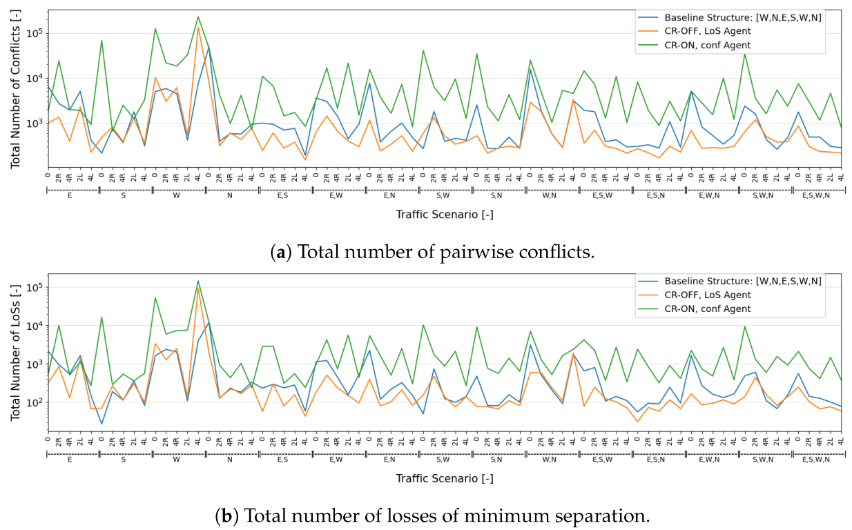
• Within traffic scenarios starting with a single direction, east and west stand out, resulting in considerably more conflicts. This justifies the emphasis by the ‘CR-ON, conf’ agent on these directions. Moreover, as expected, when aircraft are initially distributed through more directions, the consequent segmentation results in fewer conflicts and LoSs.
• It was hypothesized that increasing the number of turns would lead to a higher number of conflicts and LoSs. Turns lead to vertical deviations between cruising layers, and having aircraft enter and leave these layers lead to conflict situations [44]. However, within the experimental results, more turns sometimes result in fewer conflicts and LoSs. This is considered a result of additional segmentation created by vertical deviations. Aircraft become more distributed throughout the available airspace as now they also move within the transition layers. This effect appears to have had a positive impact on safety.

7.2. Testing of the RL Agent for Safety-Optimized Airspace Structuring

From the results obtained during training, we opted to utilize the ‘CR-ON, conf’ agent in the forthcoming testing verification with additional traffic scenarios. This RL agent was tested with a total of 225 traffic scenarios; 75 scenarios in each traffic density (i.e., low, medium, and high). The RL agent was previously trained within a medium traffic density; it is of interest to see how it behaved at lower and higher traffic densities. All testing episodes were different from the ones the RL agent trained in. For each traffic scenario (i.e., the combination of specific traffic density, initial direction(s), and the number of turns), three repetitions with different flight trajectories were performed. Each traffic scenario ran for an hour. However, note that the state formulation was not modified; it still only covered the first 20 min of the traffic scenario. The duration of the traffic scenario was increased to analyze the effect of having a scenario longer than the state contemplated. Additionally, a longer run allowed for a more complete analysis of the impact of employing the structure output by the RL agent vs. a fixed, uniform one. Finally, testing was performed in an environment where aircraft may change their speeds and altitudes to avoid conflicts.

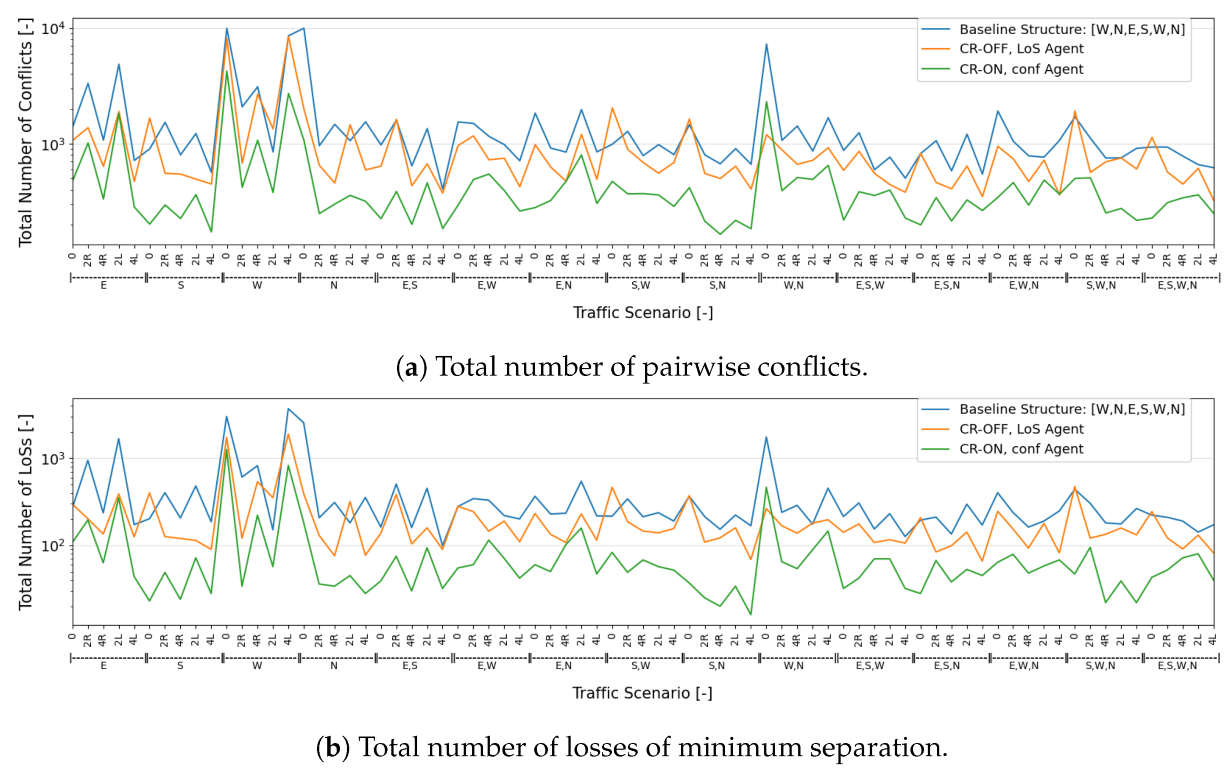
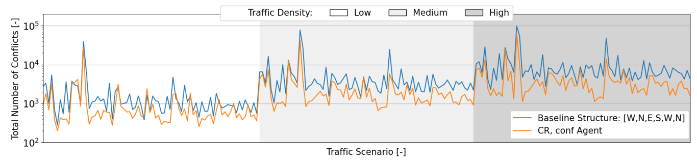
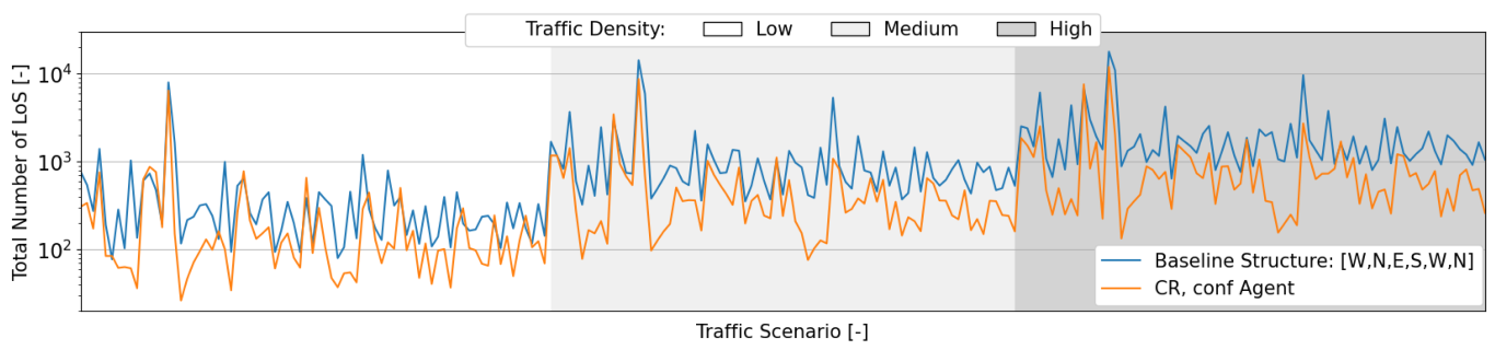
7.2.1. Safety Analysis

Figure 14 shows the mean total number of pairwise conflicts. The RL model was able to reduce the number of conflicts for all traffic scenarios and densities when compared to having one fixed airspace structure. Contrary to the hypothesized, the RL agent did not perform worse at high traffic densities. The airspace structures, which led to an optimal number of conflicts at a medium traffic density, were also applicable to higher traffic densities.

Figure 15 shows the amount of time spent with a deconflicting state decided by the CR method, instead of following their preferred state. This does not include the time to recovery when aircraft are no longer in conflict and are redirected to their next waypoints. The RL model was able to reduce the time in conflict for all traffic scenarios and densities when compared to having one fixed airspace structure. Although the RL reduced both the number of conflicts and the total time in conflict, these do not have a direct correlation. Fewer pairwise conflicts do not necessarily mean less time in conflict per aircraft and vice versa.

Figure 16 shows the mean total number of LoSs. The RL model was able to reduce the number of LoSs for all traffic scenarios and densities when compared to having one fixed airspace structure. Although the focus of the RL agent was to reduce conflicts, fewer conflicts led to fewer LoSs. Analogously to the total number of pairwise conflicts (see Figure 14), there was no decrease in efficiency for higher traffic densities. Interestingly, in comparison with the fixed structure, the improvement obtained with the RL agent appeared stronger in the high traffic density than in the low one.

Figure 17 displays the intrusion severity. For most traffic scenarios, there was no relevant discrepancy between the fixed, uniform structure, and the structure output by the RL agent. However, with the former, there were outliers where the mean intrusion severity reached higher values. With a more efficient segmentation, aircraft were better at keeping a safer distance and were not as close.

Figure 18 presents the relative speed between aircraft in an LoS situation. Higher relative speeds indicate speed heterogeneity that increased complexity in the airspace. Transition layers were in place to minimize the effect of high relative speeds from aircraft exiting and entering a cruising layer; aircraft only decelerate, turn, and accelerate within the slow layers. Slow layers are considered safer for this state change, as they are expected to be (almost) depleted of aircraft. This might not be the case when multiple aircraft initiate vertical deviations simultaneously. Additionally, a high relative speed can occur in a fast layer. Aircraft performing an avoidance maneuver in close proximity with different avoidance speeds will result in high relative speed conflict situations. On average, the structure output by the RL agent leads to a lower relative speed between aircraft in conflict. However, surprisingly, at lower traffic densities, there are outliers of high relative speeds. This may explain why, in some low-density traffic scenarios, the RL agent was not able to considerably decrease the number of LoSs (see Figure 16).

Figure 19 and Figure 20 show where LoSs occurred for all traffic scenarios tested for the fixed structure and the structures produced by the RL agent, respectively. As shown in Figure 16, with the RL agent, there were fewer LoSs. Figure 19 shows that, with the uniform structure, most of the LoSs occurred in the transition layers. Figure 20 also displays LoSs in the transition layers, but not as predominantly. In this case, the last layer stands out as having the most LoSs. This is due to the safeguard implemented on the structure output by the RL agent; if not all directions are included in the structure, the last layer is overwritten to allow for the missing directions. Consequently, this layer may have an agglomeration of aircraft with different headings, leading to a high incidence of LoSs. As per Figure 11, the RL agent opted for heavily prioritizing certain directions, instead of a more uniform distribution. This approach proves more reasonable in the medium traffic density that the RL agent was trained in than in a higher traffic density. In a medium traffic density, including multiple directions in one layer may still result in a number of conflicts that do not cancel out the benefit of prioritizing other directions. However, at high traffic densities, a high incidence of traffic in one layer may result in a significant number of conflict chain reactions with a negative impact on safety.

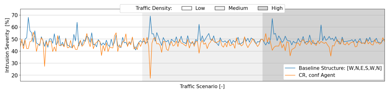
7.2.2. Stability Analysis

Figure 21 displays the mean DEP value. A high positive value represents conflict chain reactions, resulting from conflict avoidance maneuvers, causing airspace instability. Previous work on unconstrained airspace showed that applying conflict resolution maneuvers at high traffic densities tends to create secondary conflicts while reducing LoSs [25]. When free airspace is scarce, having aircraft moving laterally and occupying a larger area of airspace often results in more conflicts. However, in this work, as resolution maneuvers only move aircraft to a vertical layer dedicated to this purpose, they did not lead to secondary conflicts. For most simulated traffic scenarios, employing conflict resolution reduced the number of conflicts compared to a situation without CR.

Figure 21 shows peaks very close to both −1 and 1, showing how the effect on the stability of applying conflict resolution must be correlated with the traffic scenario and flight routes. Additionally, the RL model selects a different structure for every traffic scenario. Some structures may put stress in some traffic layers, which may create conflict ‘hotspots’ with aircraft continuously resolving and creating conflicts. Interestingly, the highest peaks (i.e., traffic scenarios in which conflict resolution induced instability) were more frequent at the lower traffic densities. Negative peaks, where conflict resolution strongly reduced the number of conflicts and occurred more often at higher traffic densities. From these results, it can be derived that the greatest benefit of conflict resolution was the decrease in conflict ‘hotspots’ resulting from the high incidence of traffic on the same ‘road’. While it can be expected that vertical conflict resolution may result in secondary conflicts, due to uncertainty regarding the intruder’s maneuvers, it reduces the number of aircraft cruising at the traffic layer by moving some aircraft to the ‘fast’ layer. At higher traffic densities, the latter effect significantly reduces the number of conflicts. At low traffic densities, conflict ‘hotspots’ are not as common and, therefore, secondary conflicts due to vertical deviations increase in the total number of conflicts.

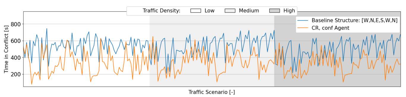
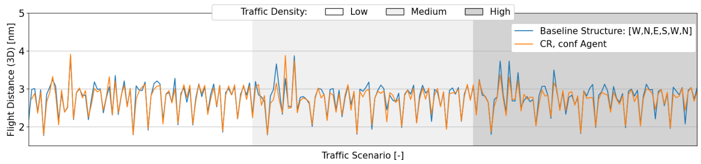
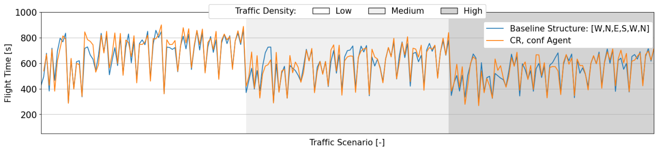
7.2.3. Efficiency Analysis

Figure 22 shows the average length of the 3D flight path per aircraft. The differences in flight paths between different structures originate mainly from: (1) different vertical distances between traffic layers that aircraft occupy throughout their paths, and (2) different numbers of vertical maneuvers to avoid conflicts. The RL model shows a reduction in the flight path lengths for some of the traffic scenarios when compared to having one fixed, uniform airspace structure; however, this behavior is not consistent throughout all traffic scenarios.

Figure 23 shows the average flight time per aircraft. There is no clear improvement in flight time when the RL model is employed. Additionally, the flight path and time are not directly proportional (see Figure 22). A shorter flight path does not necessarily mean a shorter flight time, as sometimes speed changes resulting from conflict avoidance maneuvers also affect flight time.

8. Discussion

Using reinforcement learning to find an airspace structure that catered to the traffic scenario had a positive effect by reducing the total number of conflicts and losses of minimum separation when compared to using a uniform, fixed heading distribution per vertical layer. The latter is optimal for uniform traffic distribution. However, this is hardly the case in an urban environment where aircraft must respect the topology of static obstacles (e.g., buildings, trees). Adapting the airspace to the operational traffic scenario allows for maximizing the efficiency with which the available airspace is utilized. When an inadequate structure is employed, the vertical distribution of traffic will be uneven, decreasing the intrinsic safety provided by the layered design.

However, there are still questions regarding this implementation. First, the final structure output by the RL agent seems to be directly correlated with the behavior of the conflict resolution algorithm. Structures lose efficacy severely when applied in an environment without conflict resolution. Analogously, it is likely that the structures would be less than optimal when different conflict resolution rules are implemented. Which structures benefit capacity is entirely dependent on the conditions of the operational environment. Second, it is not yet clear how the safety of operations can be guaranteed during configuration changes. Traffic scenarios will naturally vary substantially throughout the day; therefore, the airspace structure should also. In this work, changing from one structure to another was not analyzed. It was assumed that such transitions would entail several vertical deviations in order for cruising aircraft to adapt to the new structure. Increasing the number of vertical deviations may increase the number of conflicts. Thus, it is likely that, during a direct change in the airspace structure, the RL agent must take into account the previous structure to reduce the number of vertical deviations. The following sub-sections dwell further into these subjects.

8.1. Efficacy of Reinforcement Learning

As initially hypothesized, the structure outputs by the RL agent are heavily dependent on whether conflict resolution is applied or not. Without conflict resolution, the airspace structure is optimized towards efficient segmentation of the existing traffic throughout the available airspace. With conflict resolution, structures focus on increasing segmentation for the directions where most conflicts remain after conflict resolution is applied. The structures are dependent on the topology of the environment and the conflict resolution strategies that are applied. With different conditions, these structures may not be as optimal. In conclusion, as is the case with most reinforcement learning research, the RL model performs better during testing when trained in a similar environment. The conflict resolution and navigation rules with which the RL agent is trained should therefore be as similar to the real environment as possible.

Furthermore, the reward formulation heavily influences the performance of the reinforcement learning agent. It is often considered that the reward should specify what the agent should be doing, but not how it should be doing it [46]. The reward should be based on the number of LoSs as this is the paramount value for safety. However, in an environment with conflict resolution, it is often the case that the number of LoSs is not sufficient to provide enough information for proper training. Conflict resolution is often able to resolve most LoSs, and the ones remaining may not be preventable with the airspace structure alone. Thus, the RL agent will not be able to find any clear path through optimization. On the basis of the test results, with conflict resolution, the number of conflicts proved to be a more efficient reward formulation. Naturally, this is only valid because it is fair to assume that fewer conflicts will lead to fewer LoSs. Interestingly, the opposite was true for training without conflict resolution, where a reward formulation based on the LoSs resulted in faster and more optimized training. In this case, the airspace structure had a direct impact on the number of LoSs as these were not resolved by a conflict resolution algorithm. Therefore, the reward formulation should be carefully tuned to the environment.

8.2. Conflict Resolution

Previous work on layered airspace structures in urban environments focused on speed-only conflict resolution [4,44]. However, this was found insufficient to prevent conflicts at high traffic densities. As was the case with this work, conflict resolution through heading variation is often not possible. To do so would require knowing the width of every ‘road’ in order to decide where aircraft can resolve conflicts laterally. Additionally, in a multi-conflict situation, the lateral resolution could potentially cause aircraft to push each other into the surrounding urban infrastructure. Therefore, the remaining degree of freedom is the vertical dimension. By reserving vertical space for upward vertical avoidance maneuvers, we are able to reduce the total number of conflicts and losses of minimum separation. This is both due to increasing the amount of maneuvers aircraft may perform to resolve conflicts, as well as temporally increasing segmentation as some aircraft temporarily move to the layer reserved for vertical avoidance.

The results of the current study show the importance of having vertical space specifically reserved for vertical conflict resolution. The vertical maneuver will effectively resolve the conflict if: (1) the aircraft moves towards a flight level that is not already densely populated (i.e., moving vertically does not result in secondary conflicts), and/or (2) small relative speeds with aircraft present at the altitude the ownship moves into. The former is achieved by reserving the layer for vertical resolutions only. Aircraft return to the main traffic layer once the conflict has been resolved. The latter is guaranteed as the MVP employs a ‘shortest-way-out’ solution. The variation will always be as minimal as possible from the aircraft’s current state to resolve the conflict. As a result, the relative speed between aircraft traveling in the ‘fast’ layer will be relatively small as they opt for traveling as close as possible to the desired cruising speed. Thus, the relative speed with other aircraft in the ‘fast’ layer is not as great as with aircraft in the ‘slow’ layer, which is purposely used for turns that must be performed at a limited speed necessary to comply with the turn radius.

Another point of concern for the success of vertical deviation is the uncertainty regarding intruder maneuvers. In case the intruders also initiate a similar vertical maneuver, the conflict will likely not be resolved. Future research can improve on reducing uncertainty by: (1) applying priority rules defining which aircraft has the right of way; (2) sharing intent information, making aircraft aware of the intruder’s future trajectory. However, prior to using intent information, the risks of its implementation must be considered. First, data transmission and processing delays will affect aircraft reaction times, decreasing efficacy in resolving short-term conflicts. Second, the aircraft must have the necessary equipment to receive and transmit data if they want to make use of this safety. Consequently, the safety of each aircraft is also dependent on how many of its intruders have this system.

Finally, the efficacy of resolution maneuvers is dependent on the speed and acceleration of the operating aircraft. Aircraft with different performance limits will resolve a different number of conflicts. Additionally, a different number of vertical layers or different safety margins for minimum separation will affect the climbing and descending times, which may affect the number of conflicts and losses of minimum separation during vertical maneuvers. In this work, a ‘fast’ layer per traffic layer was used for conflict resolution. More layers dedicated to vertical avoidance may improve safety but it would also increase the amount of vertical layers aircraft must traverse. These choices are heavily dependent on the operational environment and aircraft involved.

8.3. Advice for Future Work

The following is advised for further research and improvements:

• The exploration of more powerful states and reward formulations. For the state formulation, four ‘snapshots’ of the evolution of the traffic were considered. However, in fast-changing traffic scenarios, the RL agent may require more snapshots to fully understand the progression of traffic over time. Additionally, only safety factors were considered as the reward. Future implementations may also benefit from including efficiency elements, such as the flight path and flight time.
• In this work, the last traffic layer was used to allow directions that the RL did not allocate space for. However, this layer may become a ‘hotspot’ for conflicts when more than one direction is set. Other possibilities could be researched (e.g., distributing aircraft traveling within “missing directions” over layers with small heading differences).

9. Conclusions

This paper examined adapting a layered airspace design to the operational traffic scenario through the use of reinforcement learning. The structures produced by an RL agent optimized the usage of airspace by segmenting aircraft efficiently throughout the available airspace by taking into account their flight plans. The results showed a reduced number of conflicts and losses of minimum separation when compared to a uniform, fixed structure, which assumed a uniform traffic scenario (as has been the case with previous research). Moreover, the introduction of layers reserved for vertical avoidance maneuvers further improved the efficacy of conflict resolution.

Applying RL with different environments and rewards showed how optimal structuring is directly related to the behavior of aircraft. In an environment where aircraft actively try to resolve conflicts, focusing on prioritizing layers for specific directions reduced the total number of conflicts and LoSs. Without conflict resolution, the RL model preferred structures in which aircraft were uniformly distributed throughout the available airspace. Additionally, rewards should be carefully tuned. Safety-wise, focus may be placed on reducing the total number of conflicts and/or LoSs. Prioritization of one of these two elements, or the weights given to each, must be set in accordance with the number of occurrences during the operation.

Nevertheless, a few considerations remain before this method can be implemented in a real-world scenario. Future work should look into transitions between different structures, and the impacts on safety that may arise from the necessary vertical deviations in order for aircraft to adapt to the new structure. Finally, this work can be extended to more heterogeneous operational environments, in terms of differences in performance limits, as well as preference for efficiency over safety.

References

1. Sesar Joint Undertaking. U–Space, Supporting Safe and Secure Drone Operations in Europe; Technical Report; Sesar Joint Undertaking: Brussels, Belgium, 2020. [Google Scholar]
2. Galster, S.M.; Duley, J.A.; Masalonis, A.J.; Parasuraman, R. Air Traffic Controller Performance and Workload Under Mature Free Flight: Conflict Detection and Resolution of Aircraft Self-Separation. Int. J. Aviat. Psychol. 2001, 11, 71–93. [Google Scholar] [CrossRef]
3. Sunil, E.; Ellerbroek, J.; Hoekstra, J.; Vidosavljevic, A.; Arntzen, M.; Bussink, F.; Nieuwenhuisen, D. Analysis of Airspace Structure and Capacity for Decentralized Separation Using Fast-Time Simulations. J. Guid. Control. Dyn. 2017, 40, 38–51. [Google Scholar] [CrossRef]
4. Doole, M.; Ellerbroek, J.; Knoop, V.L.; Hoekstra, J.M. Constrained Urban Airspace Design for Large-Scale Drone-Based Delivery Traffic. Aerospace 2021, 8, 38. [Google Scholar] [CrossRef]
5. Gunarathna, U.; Xie, H.; Tanin, E.; Karunasekara, S.; Borovica-Gajic, R. Real-Time Lane Configuration with Coordinated Reinforcement Learning. In Proceedings of the Machine Learning and Knowledge Discovery in Databases: Applied Data Science Track, Ghent, Belgium, 14–18 September 2020; Dong, Y., Mladenić, D., Saunders, C., Eds.; Springer International Publishing: Cham, Switzerland, 2021; pp. 291–307. [Google Scholar]
6. Chu, K.F.; Lam, A.Y.; Li, V.O. Dynamic lane reversal routing and scheduling for connected autonomous vehicles. In Proceedings of the 2017 International Smart Cities Conference (ISC2), Wuxi, China, 14–17 September 2017; pp. 1–6. [Google Scholar] [CrossRef]
7. Cai, M.; Xu, Q.; Chen, C.; Wang, J.; Li, K.; Wang, J.; Wu, X. Multi-Lane Unsignalized Intersection Cooperation with Flexible Lane Direction Based on Multi-Vehicle Formation Control. IEEE Trans. Veh. Technol. 2022, 71, 5787–5798. [Google Scholar] [CrossRef]
8. Standfuß, T.; Gerdes, I.; Temme, A.; Schultz, M. Dynamic airspace optimisation. CEAS Aeronaut. J. 2018, 9, 517–531. [Google Scholar] [CrossRef]
9. Schultz, M.; Reitmann, S. Machine learning approach to predict aircraft boarding. Transp. Res. Part Emerg. Technol. 2019, 98, 391–408. [Google Scholar] [CrossRef]
10. Lee, H.; Malik, W.; Jung, Y.C. Taxi-Out Time Prediction for Departures at Charlotte Airport Using Machine Learning Techniques. In Proceedings of the 16th AIAA Aviation Technology, Integration, and Operations Conference, Washington, DC, USA, 13–17 June 2016. [Google Scholar] [CrossRef]
11. Nguyen, D.D.; Rohacs, J.; Rohacs, D. Autonomous Flight Trajectory Control System for Drones in Smart City Traffic Management. ISPRS Int. J. Geo Inf. 2021, 10, 338. [Google Scholar] [CrossRef]
12. Hassanalian, M.; Abdelkefi, A. Classifications, applications, and design challenges of drones: A review. Prog. Aerosp. Sci. 2017, 91, 99–131. [Google Scholar] [CrossRef]
13. Hoekstra, J.; Ellerbroek, J. BlueSky ATC Simulator Project: An Open Data and Open Source Approach. In Proceedings of the Conference: International Conference for Research on Air Transportation, Philadelphia, PA, USA, 20–24 June 2016. [Google Scholar]
14. Hoekstra, J.; van Gent, R.; Ruigrok, R. Designing for safety: The ‘free flight’ air traffic management concept. Reliab. Eng. Syst. Saf. 2002, 75, 215–232. [Google Scholar] [CrossRef]
15. Ribeiro, M.; Ellerbroek, J.; Hoekstra, J. Review of conflict resolution methods for manned and unmanned aviation. Aerospace 2020, 7, 79. [Google Scholar] [CrossRef]
16. Lillicrap, T.P.; Hunt, J.J.; Pritzel, A.; Heess, N.; Erez, T.; Tassa, Y.; Silver, D.; Wierstra, D. Continuous control with deep reinforcement learning. In Proceedings of the 4th International Conference on Learning Representations, ICLR 2016—Conference Track Proceedings. International Conference on Learning Representations, ICLR; San Juan, Puerto Rico, 2–4 May 2016. Available online: http://xxx.lanl.gov/abs/1509.02971 (accessed on 1 November 2021).
17. Degas, A.; Islam, M.R.; Hurter, C.; Barua, S.; Rahman, H.; Poudel, M.; Ruscio, D.; Ahmed, M.U.; Begum, S.; Rahman, M.A.; et al. A Survey on Artificial Intelligence (AI) and eXplainable AI in Air Traffic Management: Current Trends and Development with Future Research Trajectory. Appl. Sci. 2022, 12, 1295. [Google Scholar] [CrossRef]
18. Brito, I.R.; Murca, M.C.R.; d’Oliveira, M.; Oliveira, A.V. A Machine Learning-based Predictive Model of Airspace Sector Occupancy. In Proceedings of the AIAA Aviation 2021 Forum, Online, 2–6 August 2021. [Google Scholar] [CrossRef]
19. Li, B.; Du, W.; Zhang, Y.; Chen, J.; Tang, K.; Cao, X. A Deep Unsupervised Learning Approach for Airspace Complexity Evaluation. IEEE Trans. Intell. Transp. Syst. 2021, 1–13. [Google Scholar] [CrossRef]
20. Wieland, F.; Rebollo, J.; Gibbs, M.; Churchill, A. Predicting Sector Complexity Using Machine Learning. In Proceedings of the AIAA Aviation 2022 Forum, Las Vegas, NV, USA, 24–26 October 2022. [Google Scholar] [CrossRef]
21. Xue, M. Airspace Sector Redesign Based on Voronoi Diagrams. J. Aerosp. Comput. Inf. Commun. 2009, 6, 624–634. [Google Scholar] [CrossRef]
22. Kulkarni, S.; Ganesan, R.; Sherry, L. Static sectorization approach to dynamic airspace configuration using approximate dynamic programming. In Proceedings of the 2011 Integrated Communications, Navigation, and Surveillance Conference Proceedings, Herndon, VA, USA, 10–12 May 2011; pp. J2-1–J2-9. [Google Scholar] [CrossRef]
23. Tang, J.; Alam, S.; Lokan, C.; Abbass, H.A. A multi-objective approach for Dynamic Airspace Sectorization using agent based and geometric models. Transp. Res. Part Emerg. Technol. 2012, 21, 89–121. [Google Scholar] [CrossRef]
24. Irvine, R. The GEARS Conflict Resolution Algorithm; Technical Report; EUROCONTROL: Brussels, Belgium, 1997. [Google Scholar] [CrossRef]
25. Tra, M.; Sunil, E.; Ellerbroek, J.; Hoekstra, J. Modeling the Intrinsic Safety of Unstructured and Layered Airspace Designs. In Proceedings of the Twelfth USA/Europe Air Traffic Management Research and Development Seminar, Seattle, WA, USA, 27–30 June 2017. [Google Scholar]
26. Sunil, E.; Hoekstra, J.; Ellerbroek, J.; Bussink, F.; Nieuwenhuisen, D.; Vidosavljevic, A.; Kern, S. Metropolis: Relating Airspace Structure and Capacity for Extreme Traffic Densities. In Proceedings of the ATM Seminar 2015, 11th USA/EUROPE Air Traffic Management R&D Seminar, Baltimore, MD, USA, 27–30 June 2005. [Google Scholar]
27. Samir Labib, N.; Danoy, G.; Musial, J.; Brust, M.R.; Bouvry, P. Internet of Unmanned Aerial Vehicles—A Multilayer Low-Altitude Airspace Model for Distributed UAV Traffic Management. Sensors 2019, 19, 4779. [Google Scholar] [CrossRef] [PubMed]
28. Cho, J.; Yoon, Y. Extraction and Interpretation of Geometrical and Topological Properties of Urban Airspace for UAS Operations. In Proceedings of the ATM Seminar 2019, 13th USA/EUROPE Air Traffic Management R&D Seminar, Vienna, Austria, 17–21 June 2019. [Google Scholar]
29. Henderson, P.; Islam, R.; Bachman, P.; Pineau, J.; Precup, D.; Meger, D. Deep Reinforcement Learning that Matters. In Proceedings of the Thirthy-Second AAAI Conference on Artificial Intelligence (AAAI-18); New Orleans, LA, USA, 2–7 February 2018. Available online: http://xxx.lanl.gov/abs/1709.06560 (accessed on 1 January 2021).
30. Tang, C.; Lai, Y.C. Deep Reinforcement Learning Automatic Landing Control of Fixed-Wing Aircraft Using Deep Deterministic Policy Gradient. In Proceedings of the 2020 International Conference on Unmanned Aircraft Systems (ICUAS), Athens, Greece, 1–4 September 2020; pp. 1–9. [Google Scholar] [CrossRef]
31. Tsourdos, A.; Dharma Permana, I.A.; Budiarti, D.H.; Shin, H.S.; Lee, C.H. Developing Flight Control Policy Using Deep Deterministic Policy Gradient. In Proceedings of the 2019 IEEE International Conference on Aerospace Electronics and Remote Sensing Technology (ICARES), Yogyakarta, Indonesia, 17–18 October 2019; pp. 1–7. [Google Scholar] [CrossRef]
32. Wen, H.; Li, H.; Wang, Z.; Hou, X.; He, K. Application of DDPG-based Collision Avoidance Algorithm in Air Traffic Control. In Proceedings of the 2019 12th International Symposium on Computational Intelligence and Design (ISCID), Hangzhou, China, 14–15 December 2019; Volume 1, pp. 130–133. [Google Scholar] [CrossRef]
33. Duan, Y.; Chen, X.; Edu, C.X.B.; Schulman, J.; Abbeel, P.; Edu, P.B. Benchmarking Deep Reinforcement Learning for Continuous Control. In Proceedings of the International Conference on Machine Learning, New York, NY, USA, 20–22 June 2016. [Google Scholar] [CrossRef]
34. Islam, R.; Henderson, P.; Gomrokchi, M.; Precup, D. Reproducibility of Benchmarked Deep Reinforcement Learning Tasks for Continuous Control. In Proceedings of the Reproducibility in Machine Learning Workshop, ICML’17, Sydney, Australia, 6–11 August 2017. [Google Scholar] [CrossRef]
35. Uhlenbeck, G.E.; Ornstein, L.S. On the theory of the Brownian motion. Phys. Rev. 1930, 36, 823–841. [Google Scholar] [CrossRef]
36. Boeing, G. OSMnx: New methods for acquiring, constructing, analyzing, and visualizing complex street networks. Comput. Environ. Urban Syst. 2017, 65, 126–139. [Google Scholar] [CrossRef]
37. Paielli, R.A. Tactical conflict resolution using vertical maneuvers in en route airspace. J. Aircr. 2008, 45, 2111–2119. [Google Scholar] [CrossRef]
38. Alejo, D.; Conde, R.; Cobano, J.; Ollero, A. Multi-UAV collision avoidance with separation assurance under uncertainties. In Proceedings of the 2009 IEEE International Conference on Mechatronics, Malaga, Spain, 14–17 April 2009; IEEE: Piscataway, NJ, USA, 2009. [Google Scholar] [CrossRef]
39. Fiorini, P.; Shiller, Z. Motion Planning in Dynamic Environments Using Velocity Obstacles. Int. J. Robot. Res. 1998, 17, 760–772. [Google Scholar] [CrossRef]
40. Chakravarthy, A.; Ghose, D. Obstacle avoidance in a dynamic environment: A collision cone approach. IEEE Trans. Syst. Man Cybern. Part A Syst. Hum. 1998, 28, 562–574. [Google Scholar] [CrossRef]
41. Velasco, G.; Borst, C.; Ellerbroek, J.; van Paassen, M.M.; Mulder, M. The Use of Intent Information in Conflict Detection and Resolution Models Based on Dynamic Velocity Obstacles. IEEE Trans. Intell. Transp. Syst. 2015, 16, 2297–2302. [Google Scholar] [CrossRef]
42. Hoekstra, J.M. Free Flight in a Crowded Airspace? Available online: https://www.semanticscholar.org/paper/Free-Flight-in-a-Crowded-Airspace-Hoekstra/9b85d3bd167044d479a11a98aa510e92b66af87b (accessed on 1 November 2021).
43. Golding, R. Metrics to Characterize Dense Airspace Traffic; Technical Report 004; Altiscope: Beijing, China, 2018. [Google Scholar]
44. Ribeiro, M.; Ellerbroek, J.; Hoekstra, J. Velocity Obstacle Based Conflict Avoidance in Urban Environment with Variable Speed Limit. Aerospace 2021, 8, 93. [Google Scholar] [CrossRef]
45. Bilimoria, K.; Sheth, K.; Lee, H.; Grabbe, S. Performance evaluation of airborne separation assurance for free flight. In Proceedings of the 18th Applied Aerodynamics Conference, Denver, CO, USA, 14–17 August 2000; American Institute of Aeronautics and Astronautics: Reston, VA, USA, 2000. [Google Scholar] [CrossRef]
46. Sutton, R.S.; Barto, A.G. Reinforcement Learning: An Introduction; MIT Press: Cambridge, MA, USA, 2018. [Google Scholar]
Figure 1. Evenly distributed airspace structure; the total heading range (360 ) is divided per the available traffic layers.
Aerospace 09 00420 g001
Figure 2. State formulation of the reinforcement learning agent. The first 16 state variables represent the expected traffic intensity per direction (east, south, west, and north) at the expected point in time. The last six positions represent the current number of aircraft in each traffic layer.
Aerospace 09 00420 g002
Figure 3. Action array output by the reinforcement learning model. Each successive four positions represent a traffic layer. The highest integer value indicates the direction (east, south, west, or north) to be allowed in the respective layer.
Aerospace 09 00420 g003
Figure 4. The urban environment used in these experiments. The data were retrieved from the OSMnx python library [36]. Nodes are highlighted in blue.
Aerospace 09 00420 g004
Figure 5. Possible directions in each one of six available traffic layers: W (west), N (north), E (east), and S (south).
Aerospace 09 00420 g005
Figure 6. Different altitude layers used in this work.
Aerospace 09 00420 g006
Figure 7. Representation of a velocity obstacle (VO) imposed by intruder B, and the relationship between a circular velocity vector set and the protected zone (PZ) [41]. By adding the intruder’s velocity, the collision cone (CC) is translated, forming the intruder’s VO.
Aerospace 09 00420 g007
Figure 8. Modified voltage potential (MVP) geometric resolution. Adapted from [14].
Aerospace 09 00420 g008
Figure 9. Evolution during training of two RL agents—one trained based on the number of conflicts (in blue) and the other on the number of LoSs (in orange). Conflict resolution was not applied in this environment.
Aerospace 09 00420 g009
Figure 10. Evolution during training of two RL agents, one trained based on the number of conflicts (in blue) and the other on the number of LoSs (in orange). Conflict resolution was applied in this environment.
Aerospace 09 00420 g010
Figure 11. Example of airspace structure output by the two best-performing RL agents. On the left: the RL agent trained without CR, based on the number of LoSs. On the right: the RL agent trained with CR, based on the number of conflicts.
Aerospace 09 00420 g011
Figure 12. Final comparison of the best RL agents during training in an environment without conflict resolution. The results are directly compared using a baseline, fixed structure.
Aerospace 09 00420 g012
Figure 13. Final comparison of the best RL agents during training in an environment with conflict resolution. The results are directly compared using a baseline, fixed structure.
Aerospace 09 00420 g013
Figure 14. Mean total number of pairwise conflicts during testing of the RL agent. All traffic densities had 75 traffic scenarios, with the initial direction(s) and the number of turns following the same order as shown during the training phase.
Aerospace 09 00420 g014
Figure 15. Total time in conflict per aircraft. All traffic densities had 75 traffic scenarios, with the initial direction(s) and the number of turns following the same order as shown during the training phase.
Aerospace 09 00420 g015
Figure 16. Mean total number of losses of separation. All traffic densities have 75 traffic scenarios, with the initial direction(s) and the number of turns following the same order as shown during the training phase.
Aerospace 09 00420 g016
Figure 17. Mean intrusion severity rate. All traffic densities had 75 traffic scenarios, with the initial direction(s) and the number of turns following the same order as shown during the training phase.
Aerospace 09 00420 g017
Figure 18. Mean relative speed between pairs of aircraft during LoSs with multiple layers. All traffic densities had 75 traffic scenarios, with the initial direction(s) and the number of turns following the same order as shown during the training phase.
Aerospace 09 00420 g018
Figure 19. Altitudes at which LoSs occur with a baseline structure. The sizes of the points vary between a maximum value of 3128 and a minimum value of 1 LoS. All traffic densities have 75 traffic scenarios, with the initial direction(s) and the number of turns following the same order as shown during the training phase.
Aerospace 09 00420 g019
Figure 20. Altitudes at which LoSs occurred with the structure produced by the RL agent. The sizes of the points vary between a maximum value of 7519 and a minimum value of 1 LoS. All traffic densities had 75 traffic scenarios, with the initial direction(s) and the number of turns following the same order as shown during the training phase.
Aerospace 09 00420 g020
Figure 21. Domino effect parameter values. All traffic densities have 75 traffic scenarios, with the initial direction(s) and the number of turns following the same order as shown during the training phase.
Aerospace 09 00420 g021
Figure 22. Flight path per aircraft. All traffic densities had 75 traffic scenarios, with the initial direction(s) and the number of turns following the same order as shown during the training phase.
Aerospace 09 00420 g022
Figure 23. Flight time per aircraft. All traffic densities had 75 traffic scenarios, with the initial direction(s) and the number of turns following the same order as shown during the training phase.
Aerospace 09 00420 g023