Aerodynamic Performance Uncertainty Analysis and Optimization of a Conventional Axisymmetric Vehicle Based on Parallel Polynomial Chaos Expansions

Abstract

In this study, the aerodynamic uncertainty analysis and optimization of a conventional axisymmetric vehicle with an aerodynamic configuration were investigated. The prediction precision of the typical aerodynamic performance estimating methods, namely, engineering estimation and numerical simulation, was compared using the wind tunnel test data of the vehicle. Then, using a modified missile data compendium (DATCOM) software, a high-efficiency and high-precision method was developed, which was applied to analyze and characterize the aerodynamic parameters of the axisymmetric vehicle. To enhance the robustness and reliability of aerodynamic performance, an uncertainty-based design optimization (UDO) framework was established. The design space was scaled by parameter sensitivity analysis, and improved computational efficiency was achieved by developing parallel polynomial chaos expansions (PCEs). The optimized results show that the modified method exhibits high accuracy in predicting aerodynamic performance. For the same constraints, the results of the deterministic design optimization (DDO) showed that compared with the initial scheme, the probability of the controllability-to-stability ratio satisfying the constraint decreased from 98.8% to 72.4%, and this value increased to 99.9% in the case of UDO. Compared with the results of the initial scheme and DDO, UDO achieved a considerable reduction in mean values and standard deviation of aerodynamic performances, which can ensure a higher probability of constraints meeting the design requirements, thereby, realizing a reliable and robust design.

1. Introduction

In the coming decades, physical modeling and highly accurate predictions of aerodynamic performance will be the focus of vehicle research. It can be seen from current research that aerodynamic data prediction of vehicles is always based on deterministic design, which does not consider the errors and uncertainties of physical models, accidental uncertainties caused by natural variables, and errors or uncertainties from test data. The precision of long-range strike weapons and the design of new axisymmetric vehicles require robust and reliable aerodynamic data. Therefore, research should focus on potential uncertainties in aerodynamic prediction and optimization, such as the dimensional deviations between the physical model and the actual vehicle, errors in the numerical model, actual flight conditions, etc.

Several studies have investigated various uncertainty factors in aerodynamic experiments and numerical calculations. Burner et al. [1] supplemented uncertainty analyses with assessments of experimental errors, and the utilization of experimental methods with modern designs, which helped explore the influence of various uncertainties, such as sensors and state variables on the measurement accuracy of model pitch angle in wind tunnel tests. Some academics [2,3,4,5] focused on the influence of shape deviation on aerodynamic performance. Some recent studies have shown that deterministic designs are easily influenced by uncertainties in certain geometric variables or environmental parameters [6]. Moreover, there are many uncertain factors, such as the uncertainty of model assumptions, when using a mathematical model to represent a physical process. Some details of the source and classification of uncertainties in computational fluid dynamics (CFD) simulations [7,8] have been discussed. Zhang et al. [9] focused on quantifying blunt body surface thermal uncertainty, along with flow parameters, and jet geometry in the presence of free-stream perturbations. Andrea et al. explored the impact of epistemic uncertainties and CFD computational errors on aerodynamic performance [10]. These studies, however, have been limited to vehicle components or two-dimensional airfoils. More evidence is needed to determine whether local alterations considerably influence the main aerodynamic performance of vehicles. When we compare airfoil or component design with vehicle shape design, the number of design variables, and the discrepancy of feature dimensions increase considerably. The changes in variables can provide crucial insights for optimizing the acquisition of more high-fidelity data and faster prediction of data in shape design optimization. Thus, it is crucial to analyze the uncertainty of aerodynamic performance at the vehicle system level and provide clear answers.

In recent years, several scholars have conducted uncertainty analyses using methods such as the sensitivity method, moment method, Monte Carlo simulation (MCS), and polynomial chaos expansions (PCEs) [11]. The sensitivity and moment methods are suitable for a system with minuscule parameter uncertainty and an approximately linear model. The MCS method is a statistical method that can present an accurate analysis of the uncertainty of a system only after drawing large numbers of samples. The PCE method has been widely used as it can quantify and characterize uncertainty through polynomial coefficients. However, its drawback is that the chain reaction between the calculated amounts increases considerably, and the dimensions are overinflated, which is known as a “dimensional disaster”. Therefore, developing a reasonable dimensionality reduction method is an urgent problem.

The conventional (wing-tail shape) axisymmetric aerodynamic configuration is widely adopted in air vehicles, especially for supersonic air-to-air and surface-to-air missiles. This configuration can provide greater maneuvering ability while maintaining flight speed. In this study, we proposed an uncertainty-based aerodynamic shape optimization framework for a target drone—with a conventional axisymmetric aerodynamic configuration—to investigate the aerodynamic characteristics of vehicles with such configurations. Analysis and quantification of all uncertainties of the vehicle system were studied based on random theory; moreover, the influences of uncertainties on the aerodynamic performance of conventional axisymmetric aerodynamic vehicles were analyzed. The result of uncertainty-based optimization was compared with deterministic optimization and the initial scheme.

The rest of the paper is organized as follows: In Section 2, the aerodynamic profile parameters of the vehicle and flight conditions are introduced; in Section 3, the precision of the two prediction methods of aerodynamic data is compared with the wind tunnel test data, based on which a high-efficiency and high-precision method is developed, and the potential uncertainty factors are analyzed and classified sequentially; in Section 4, the parallel PCE is described and tested; in Section 5, a mathematical model of deterministic design optimization (DDO) and uncertainty-based design optimization (UDO) are introduced; in Section 6, the results of DDO and UDO are presented, followed by the comparative analysis results.

2. Description

2.1. Shape and Parameters

The vehicle examined in this study was a target drone (Figure 1), which has the typical characteristics of a conventional axisymmetric aerodynamic configuration. It has a Haack series-shaped nose cone, a cylindrical body, four trapezoidal wings, and four trapezoidal tail surfaces. The wing profile (airfoil) is hexagonal, and the tail profile (airfoil) is rhomboidal. Two rectangular cable covers run through both sides of the projectile body. The main wing is installed near the mass center of the vehicle, and the tail is installed after the main wing. There is a convex part on the belly of the vehicle, which results in the fuselage being an imperfect rotating body. The sliders are regarded as part of the fuselage without design optimization.

We used 30 geometric shape parameters and design variables to establish the axisymmetric vehicle model. Numerical variations in the vehicle’s geometric parameters directly affected the aerodynamic characteristics of the vehicle, as they changed the geometric shape of the vehicle. All shape variables of this vehicle are listed and illustrated in

Table 1. Parametric modeling of vehicle.

Design Variable	Unit	Physical Significance	Perturbation Variable	Relative Deviation	Optimization Variable	Probability Distribution
LNOSE	m	Nose length	x1	±0.001	no	uniform
LCENTR	m	Fuselage length	x2	±0.001	no	uniform
DNOSE	m	Nose diameter at base	x3	±0.001	no	uniform
DCENTR	m	Fuselage diameter	x4	±0.001	no	uniform
BNOSE	m	Nose bluntness radius or radius of truncation	x5	±0.001	no	uniform
Xc	---	Mass center of vehicle	x6	±0.01	no	uniform
XLE1	m	Distance from missile nose to chord leading edge at wing root chord station	x7	±0.01	yes	uniform
SSPAN11	m	Semi-span length of wing	x8	±0.001	yes	uniform
CHORD11	m	Panel chord length at wing root chord location	x9	±0.001	yes	uniform
CHORD12	m	Panel chord length at wing tip chord location	x10	±0.001	yes	uniform
LER11	m	Leading edge radius at wing root chord station	x11	±0.001	yes	uniform
LER12	m	Leading edge radius at wing tip chord station	x12	±0.001	yes	uniform
ZUPPER11	---	Thickness-to-chord ratio of upper surface at wing root chord station	x13	±0.001	yes	uniform
ZUPPER12	---	Thickness-to-chord ratio of upper surface at wing tip chord station	x14	±0.001	yes	uniform
LMAXU11	---	Fraction of chord from leading edge to maximum thickness of upper surface at root chord station	x15	±0.001	yes	uniform
LMAXU12	---	Fraction of chord from leading edge to maximum thickness of upper surface at tip chord station	x16	±0.001	yes	uniform
LFLATU11	---	Fraction of chord of constant thickness section of upper surface at root chord station	x17	±0.001	yes	uniform
LFLATU12	---	Fraction of chord of constant thickness section of upper surface at tip chord station	x18	±0.001	yes	uniform
XLE21	m	Distance from missile nose to chord leading edge at tail root chord station	x19	±0.01	yes	uniform
XLE22	m	Distance from missile nose to chord leading edge at tail root chord station	x20	±0.01	yes	uniform
SSPAN21	m	Semi-span length of tail	x21	±0.001	yes	uniform
CHORD21	m	Panel chord length at tail root chord location	x22	±0.001	yes	uniform
CHORD22	m	Panel chord length at tail tip chord location	x23	±0.001	yes	uniform
LER21	m	Leading edge radius at tail root chord station	x24	±0.001	yes	uniform
LER22	m	Leading edge radius at tail tip chord station	x25	±0.001	yes	uniform
ZUPPER21	---	Thickness-to-chord ratio of upper surface at tail root chord station	x26	±0.002	yes	uniform
ZUPPER22	---	Thickness-to-chord ratio of upper surface at tail tip chord station	x27	±0.002	yes	uniform
THETA1	deg	setting angle of wings	x28	±1	no	uniform
THETA2	deg	setting angle of tail	x29	±1	no	uniform
Xhinge	---	Hinge axis position	x30	±0.01	no	uniform

.

2.2. Flight Conditions

The flight trajectory of the vehicle includes the take-off, climb phase, cruise phase, and dive phase (Figure 2). The design altitude of the cruise phase in this ballistic scheme is 20 km, and the design velocity is 2.1 Mach number. As a target drone, maximum flight time should be designed for the aircraft. Under the condition that the propulsion system carries a fixed mass of propellant, the time of the cruise phase can be improved by reducing propellant consumption per unit time, which can be achieved by reducing the drag in the cruise phase.

The main optimization objective of this study was to realize the design of a minimum drag in the cruise phase. There were also other implicit design conditions for this state, including the ability to provide enough lift for retaining flight altitude, flight stability, and controllability. The stability of a vehicle refers to its ability to resist the influence of disturbance, which is characterized by its longitudinal static stability. Controllability is the response characteristic of a projectile body to tail deflection, and in this study, the controllability-to-stability ratio reflects the influence of tail deflection on attitude change. Considering the mutual restrictions between static stability and maneuverability, the constraints of longitudinal static stability and the controllability-to-stability ratio were specified.

3. Aerodynamic Performance Prediction Method and System Uncertainty Factors

3.1. Methods for Estimating Aerodynamic Performance Parameters

From conceptual design to detailed design, aerodynamic characteristics considerably influence the selection of subsequent configuration parameters, such as lift force and drag force. Three prediction methods are used for aerodynamic numerical characteristics, namely, engineering estimation, numerical simulation, and wind tunnel tests. In this study, the aerodynamic performance of the vehicle was examined using wind tunnel tests under two conditions, including free-stream Mach numbers of Ma = 1.75 and 2.53. The comparison of these two sets of aerodynamic performance helps determine the errors in the aerodynamic data.

(1)

Engineering estimation

Engineering estimation is realized using missile data compendium (DATCOM) software, which adopts component combination and modular methods; this enables accurate and efficient prediction of various aerodynamic data of vehicles with traditional aerodynamic configurations [12]. DATCOM also has good adaptability and high estimation accuracy for the conventional axisymmetric configuration, and it can be used to describe various types of airframe surface projections. In DATCOM, the designer defines one vehicle shape by describing its form and the dimensional values of each part (the parameters given in Table 1) and sets the flight conditions such as flight height and Reynold’s number. For a vehicle with a specific shape, all aerodynamic performance data are obtained with an overall calculation time < 2 s, indicating the efficiency and convenience of the engineering estimation method.

(2)

Numerical simulation

Numerical simulations based on CFD are carried out using ANSYS Fluent software [13]. The 3D compressible RANS equations are solved using the shear-stress transport (SST) renormalization group K-ω turbulence model. The SST K-ω model is adopted as it has been widely used in the numerical calculation of multiple flow problems, such as airfoil boundary layer [14], supersonic vehicle design [15], supersonic flow [16], and especially in aerodynamic shape optimization [17]. The second-order upwind scheme is used for the discretization of the convective terms in all transport equations.

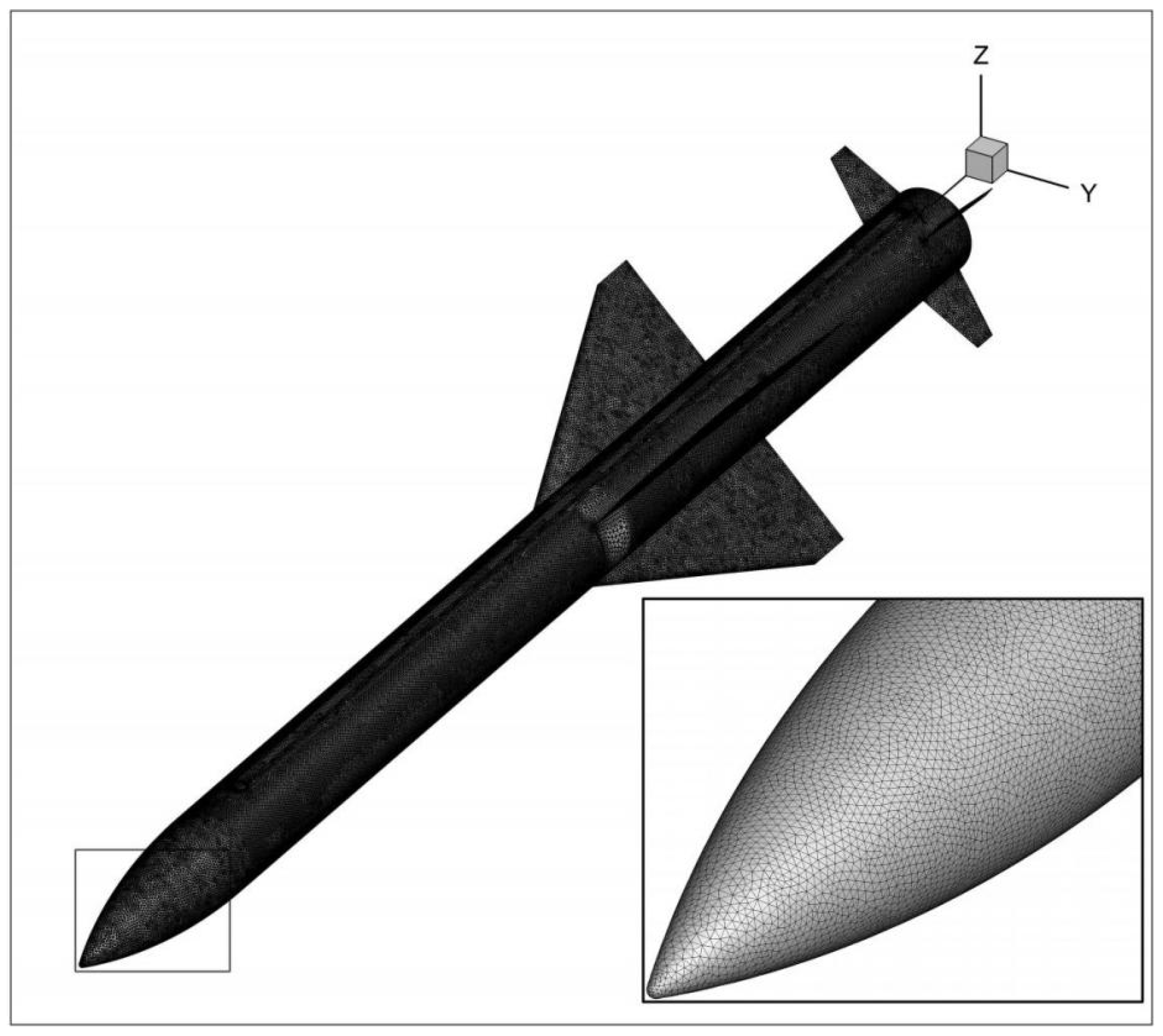
Based on the objective of this research, that is, to determine the aerodynamic values of the vehicle and calculate its aerodynamic coefficients, it is important to simplify the calculation model and only retain the features of the main components during parametric modeling in CFD. A fluent mesh was used to generate an unstructured grid in the computing domain. Grid independence was verified before further simulation to exclude the influence of the grid on numerical results (Figure 3). The numerical simulation focuses on the whole turbulent layer; therefore, there is one important relation $y^{+}=\Delta y\rho u_{\tau }/\mu$, where $\Delta y$ is the distance of the first grid point off, and $\rho ,u_{\tau },\mu$ are the density, friction velocity, and molecular viscosity, respectively. For simulating complicated flowfields, $\rho ,u_{\tau },\mu$ have different values in different flowfield regions; as a result, $\Delta y$ satisfying $y^{+}<1$ will also have different conditions [18]. $\rho ,u_{\tau },\mu$ depend on the standard atmospheric characteristics of the flight state; when y⁺ is 1, the first layer grid height of the boundary layer can be calculated as $\Delta y=1.83957\times {10}^{-6} \mathrm{m}$, which will be used as the reference value for the mesh near the vehicle surface. Grid quality directly affects the solving accuracy of numerical solutions. To ensure better calculation accuracy of models with different grid elements, the height of the first-layer wall grid corresponding to different grids is given in

Table 2. Aerodynamic coefficients under different grid numbers.

		Aerodynamic Coefficients
Number of Elements	$\mathit{\Delta }\mathit{y}$	CA	CN	CM	0 < y+ ≤ 1
1,583,795	0.0003	0.6163	3.4105	2.0957	92.13%
2,334,777	0.0002	0.6037	3.4154	2.1104	99.16%
3,981,490	0.0002	0.6019	3.4237	2.1171	99.73%
4,947,050	0.0002	0.5968	3.4129	2.1036	99.82%
6,350,802	0.00008	0.5876	3.4209	2.1094	99.90%
7,123,409	0.00008	0.5793	3.4215	2.1169	99.96%
8,562,353	0.00008	0.5766	3.4212	2.1173	100%
9,690,507	0.00008	0.5767	3.4213	2.1174	100%

. At the completion of the numerical simulation, the y⁺ of the wall surface is counted and displayed as a percentage, in which the proportion of y⁺ in the interval from 0 to 1 is the focus of attention.

Models with different degrees of grid resolution were established, and the mean pressure coefficients of the vehicle were calculated with different grid numbers. When there were 8.56 × 10⁶ unstructured grids in the computing domain, the numerical results obtained using CFD were highly accurate, and all y⁺ were in the range of 0–1, and the maximum y⁺ value was approximately 0.83. As the number of grids increased, all aerodynamic coefficients did not change substantially. The entire computing domain was set as a sphere (Figure 4), and the grid model schematic diagram of the vehicle body is as shown in Figure 5.

(3)

Wind tunnel

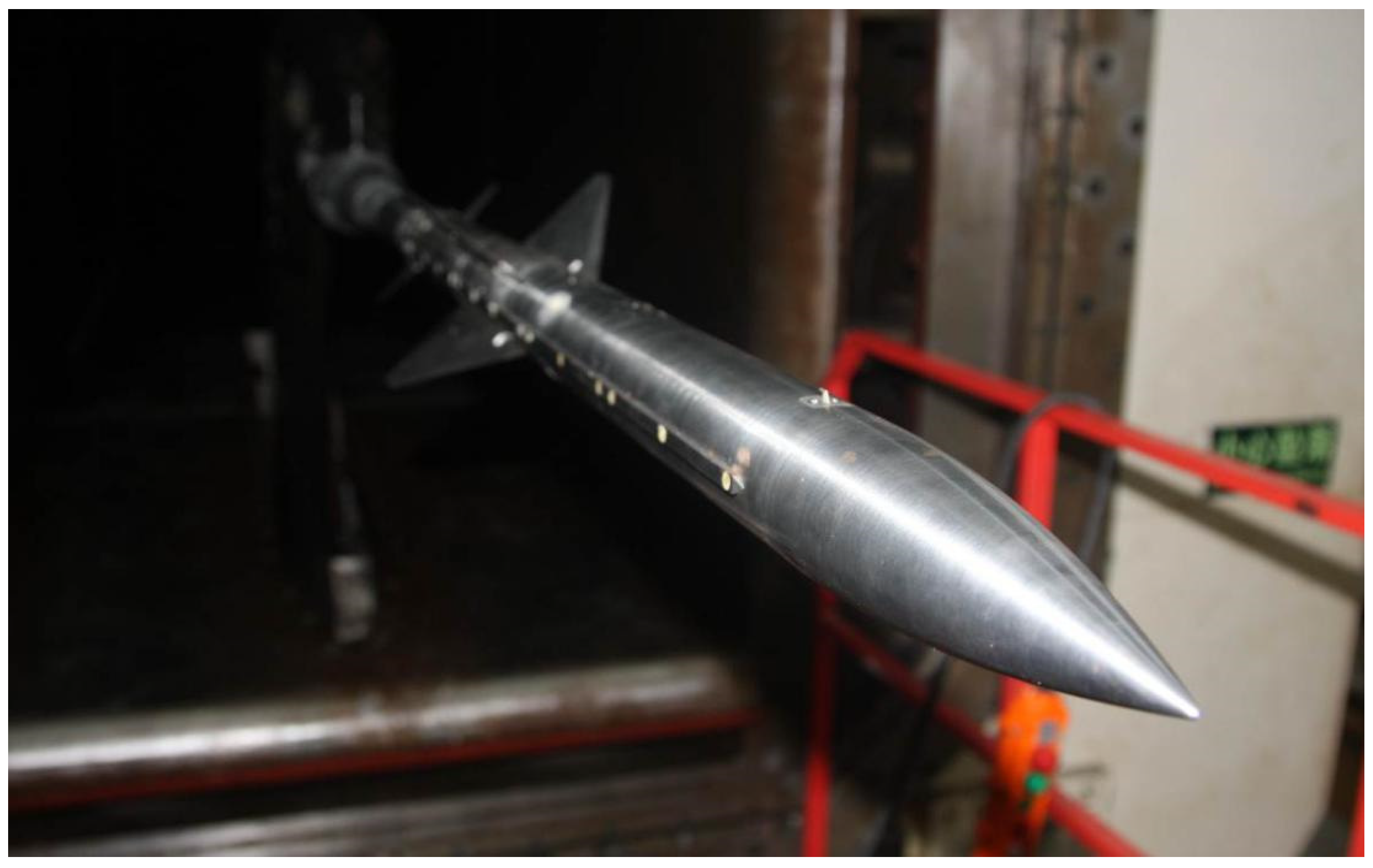
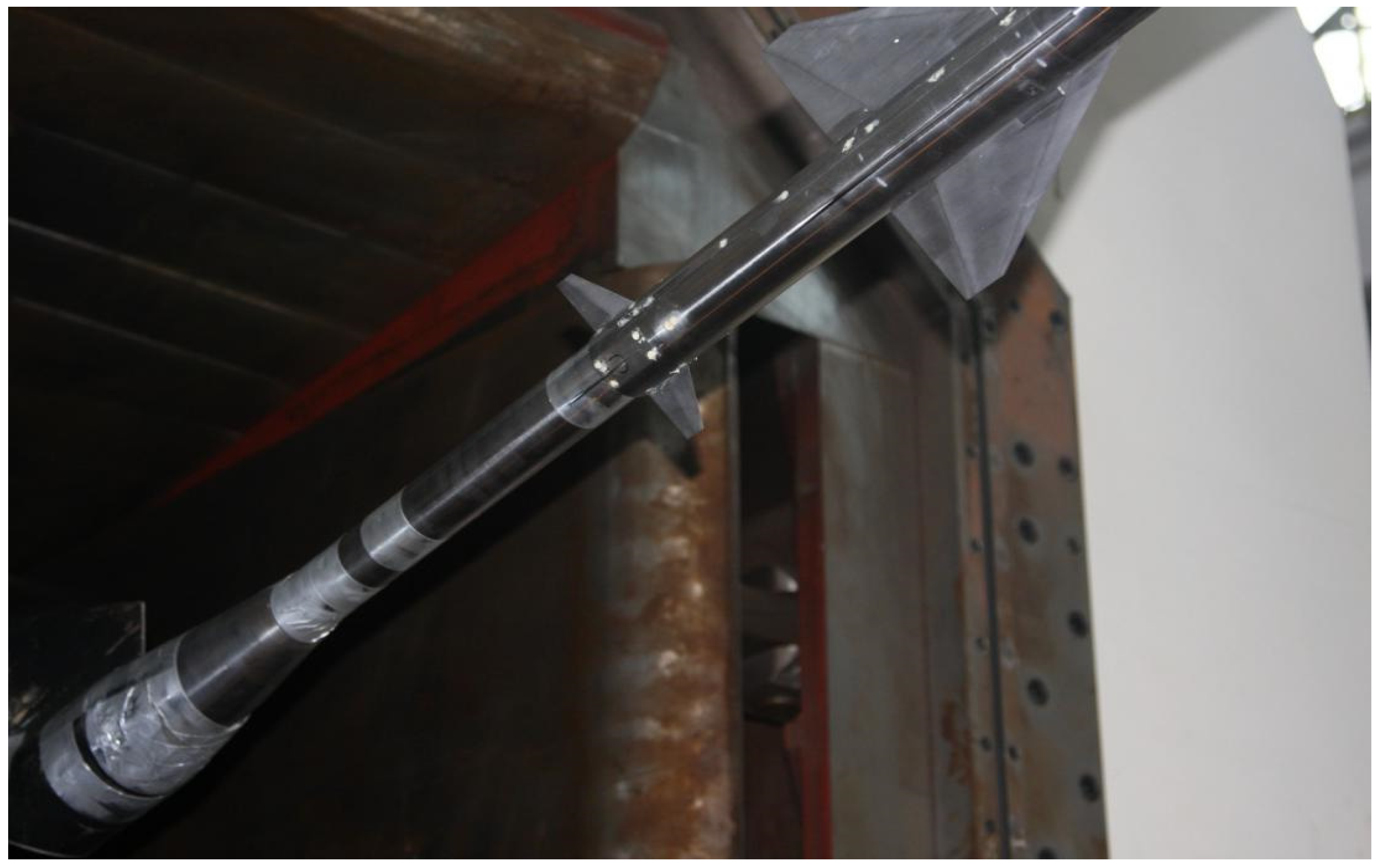
Aerodynamic tests of the vehicle were carried out in an FD12 wind tunnel built by the China Academy of Aerospace Aerodynamics. The FD12 wind tunnel test equipment had a cross-section of 1.2 m × 1.2 m and a Mach number range of Ma = 0.4–4. It belongs to the subsonic, transonic, and supersonic wind tunnels, also known as a three-sonic wind tunnel. A 1:6 physics scale model (Figure 6) was used in the wind tunnel tests using air as the test medium. The aerodynamic parameters of the vehicle were measured using wind tunnel tests at an altitude of 10 km under two conditions, i.e., free-stream Mach numbers of Ma = 1.75 and 2.53. For these tests, the flow conditions were set as follows: angle of attack (AOA) α = −2°, 0°, 2°, 4°, 6°, 8°, 11°, 14°, 17°, and 20°, and Reynolds number of Re = 8.82 × 10⁷ and 1.27 × 10⁸. The wind tunnel test adopted a support sting, as shown in Figure 7.

(4)

Comparative analysis

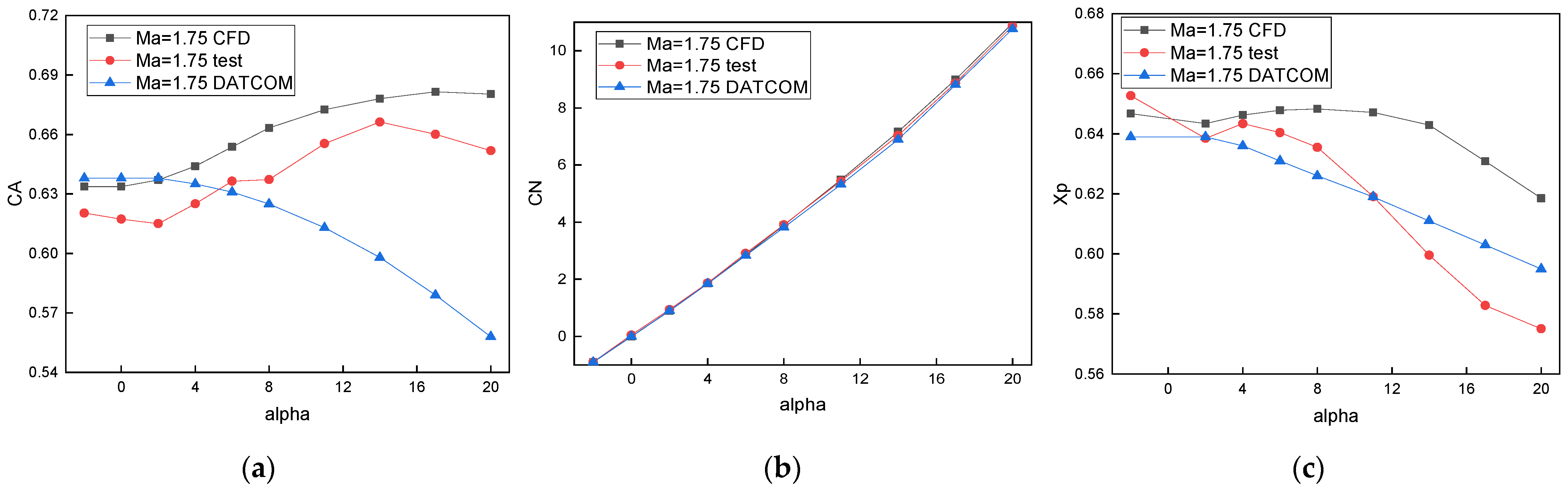
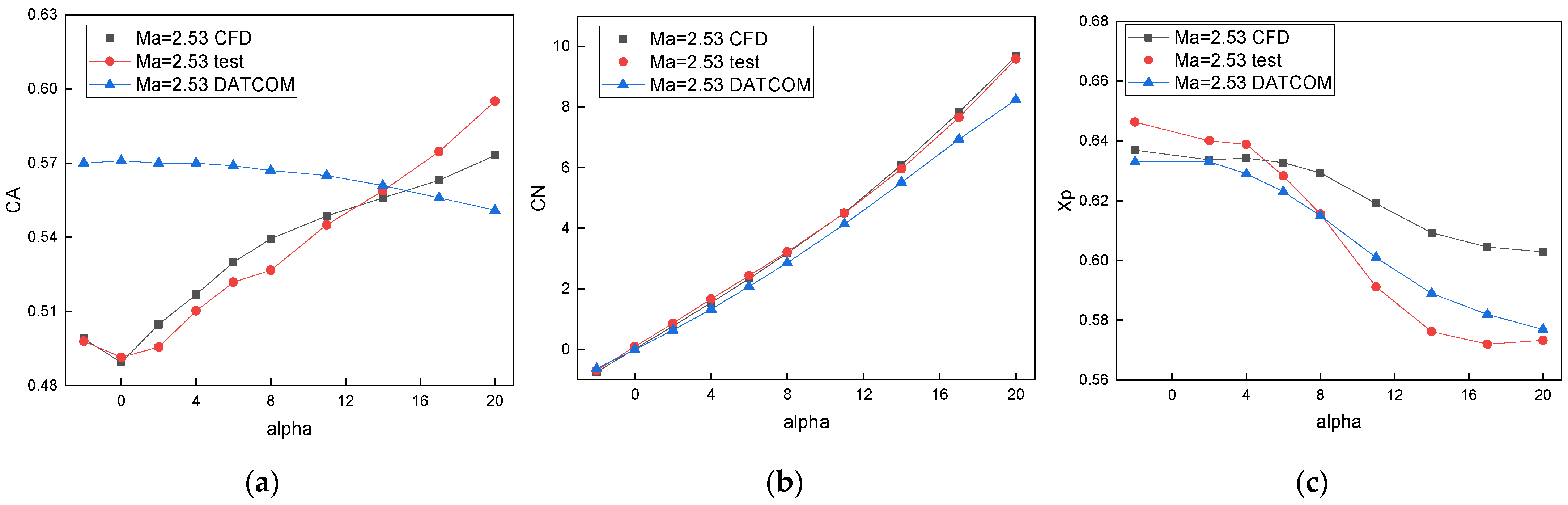
DATCOM, CFD simulations, and wind tunnel tests determined the axial force coefficient (CA), normal force coefficient (CN), and pressure core coefficient (Xp) of the axisymmetric vehicle, as shown in Figure 8 and Figure 9.

All aerodynamic coefficient data are shown in Figure 8 and Figure 9. Aerodynamic coefficient deviations due to the utilization of two computing methods were calculated. For the different Reynolds numbers, the accuracy of CFD was higher than that of DATCOM. In particular, aerodynamic coefficients and their tendency with changes in AOA were close to the wind tunnel data, based on the calculated CA and CN using CFD. The DATCOM projections were appropriate in some (e.g., the center of pressure coefficient), but not in all areas. The empirical database that underpins these forecasts of DATCOM is for a conventional vehicle without a vortical flow. Related studies have shown that Euler simulation cannot predict the flowfield correctly in similar cases, and detached eddy simulations would be a better option [19]. Due to the limitations of the turbulence model, vortex characteristics were not adequately captured. This is attributed to the appearance and disappearance of coherent eddy currents near the fuselage, which disturbs the accuracy of the pitching moment and normal force to some extent. With an increase in AOA, the calculated values of the pressure center coefficient using CFD, and wind tunnel tests show obvious deviations.

The vehicle creates a vortex near the fuselage at a Mach number of Ma = 1.75, such as a wing-tip vortex and a body-shedding vortex. With an increase in AOA, the circulation of the vortex and the vorticity increase considerably. The eddy motion causes energy loss and local pressure on the vehicle surface. This explains the differences between the values of CA predicted by DATCOM using CFD and the wind tunnel tests. This phenomenon also occurs in Ma = 2.53. The appearance of vortical flow is the primary distinction between the three prediction methods; however, this aspect is not considered in DATCOM.

(5)

Modified engineering prediction method

Based on the objective of this study to conduct uncertainty analyses on aerodynamic performance, the computational efficiency of DATCOM matched the research requirements, and the prediction accuracy of the center of pressure coefficient was satisfactory. Therefore, DATCOM was selected to obtain the aerodynamic data of the vehicle. However, there were some errors in the aerodynamic coefficient of DATCOM due to the vortex. In that case, the model for the prediction of aerodynamic data should be corrected based on the DATCOM software. In the subsequent verification of model accuracy, CFD was used as a standard to test the predicted model.

To facilitate optimization, a numerically modified engineering prediction method for force coefficient was developed using the wind tunnel test data. Considering the influence of vortical flow on the aerodynamic coefficient, CA was corrected based on the relative error between the DATCOM data and wind tunnel test data. First, a set of statistical errors $Y_e$ can be obtained based on known test data.

$$Y_e(Ma,\alpha )=\frac{C{A}_{test}(Ma,\alpha )-C{A}_{DATCOM}(M\mathrm{a},\alpha )}{C{A}_{DATCOM}(M\mathrm{a},\alpha )}$$

(1)

where Ma = 1.75 and 2.53, α = −2°, 0°, 2°, 4°, 6°, 8°, 11°, 14°, 17°, and 20°. Therefore, when Mach number and AOA are satisfied, $1.75\le Ma\le 2.53$, and $-2^{\circ }\le \alpha \le {20}^{\circ }$, respectively, the relative errors of CA ${\tilde{y}}_{CA}(Ma,\alpha )$ in different states can be obtained by interpolation.

$${\tilde{y}}_{CA}(Ma,\alpha )=\left\{\begin{array}{c}{Y}_e(Ma,{\alpha }_1)+(Y_e(Ma,{\alpha }_2)-Y_e(Ma,{\alpha }_1))\times (\alpha -{\alpha }_1)/({\alpha }_2-{\alpha }_1)\\ Y_e(M{a}_1,\alpha )+(Y_e(M{a}_2,\alpha )-Y_e(M{a}_1,\alpha ))\times (Ma-M{a}_1)/(M{a}_2-M{a}_1)\end{array}\right.$$

(2)

According to the relative error, the CA predicted by DATCOM can be corrected as:

$$C{A}_{co-DATCOM}=C{A}_{DATCOM}\times (1+{\tilde{y}}_{CA})$$

(3)

However, CN is corrected using the derivative of CN based on AOA, since the derivative of the CN calculated using wind tunnel data and DATCOM differs considerably with increase in AOA. First, the derivative of CN based on AOA was calculated, as given below:

$$\Delta CN(M\mathrm{a},\alpha )=(\frac{dC{N}_{test}(M\mathrm{a},\alpha )}{d\alpha }-\frac{dC{N}_{DATCOM}(M\mathrm{a},\alpha )}{d\alpha })/\frac{dC{N}_{DATCOM}(M\mathrm{a},\alpha )}{d\alpha }$$

(4)

Similarly, the relative error correction function of CN can be obtained by interpolation through data statistics with wind tunnel data, which is written as ${\tilde{y}}_{cn}\approx \Delta CN(M\mathrm{a},\alpha )$.

$$C{N}_{co-DATCOM,\alpha }=C{N}_{DATCOM,\alpha -1}\times (1+\frac{dC{N}_{DATCOM}}{d\alpha }\times (1+{\tilde{y}}_{cn}))$$

(5)

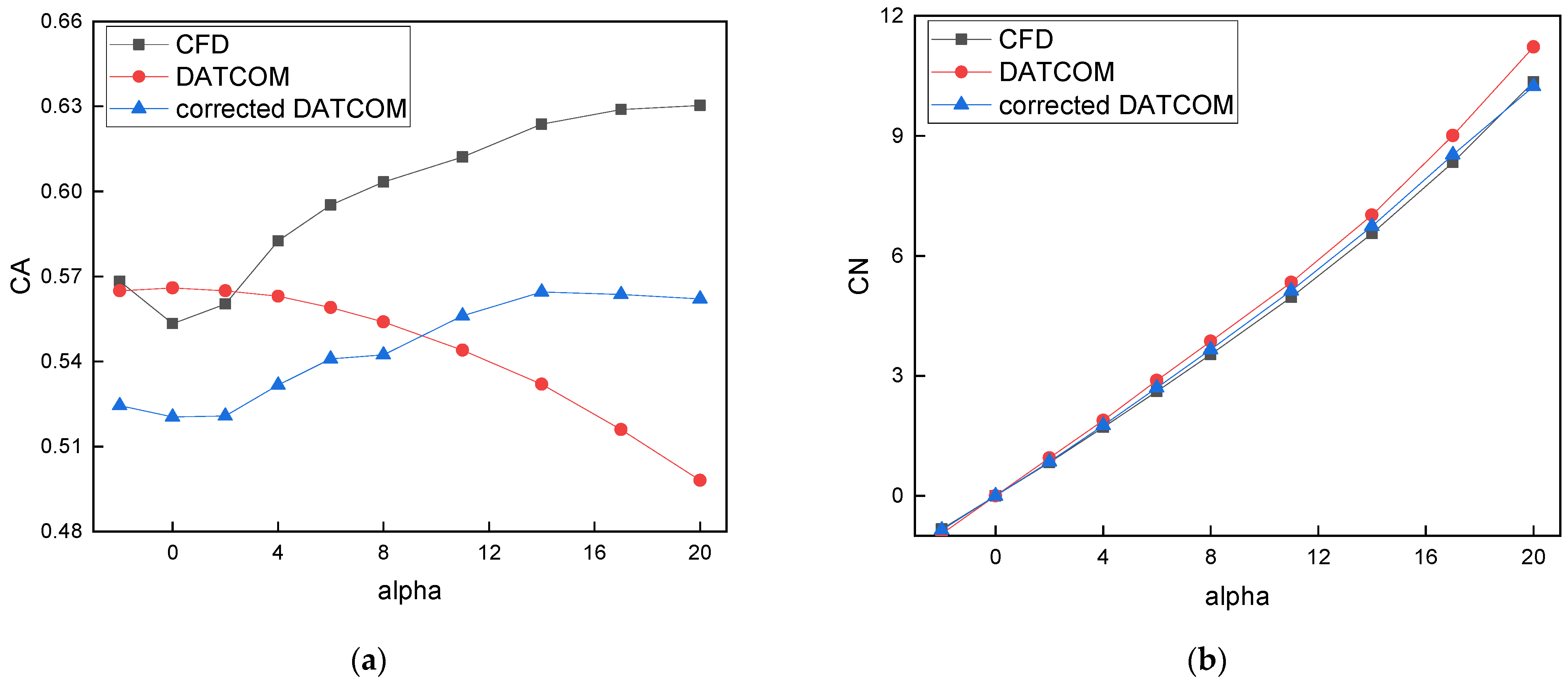
The values of CA and CN are calculated based on the modified model, as shown in Figure 10.

After the aerodynamic coefficients obtained using DATCOM were corrected, the aerodynamic coefficient values obtained by three different calculations were compared at Ma = 2.1. Experimental data were not available for this stage since the vehicle in Ma = 2.1 did not undergo wind tunnel testing. For further comparison, CFD was selected as the criteria as it performed well for both Mach numbers, Ma = 1.75 and 2.53. The CA trend predicted by the corrected DATCOM considerably improved, and it was consistent with the trend predicted by CFD. Since the CFD model also has certain errors, some value deviations were allowed. The calculation methods of uncertainty caused by the error of corrected DATCOM are presented in Section 3.2.

3.2. Source of Aerodynamic Deviations

The uncertainty analysis of aerodynamic characteristics should quantitatively evaluate the input and model uncertainties of the modified engineering prediction method. The possible errors of the input parameters can be roughly divided into the following categories: the errors and uncertainties of physical modeling and random aerodynamic interference during flight conditions. The model uncertainties are mainly attributed to the errors in the engineering prediction method.

(1)

Input uncertainties

Compared with the real final product of the vehicle, there are many errors and deviations with the geometric shape parameters in one physical vehicle model due to the processes of manufacturing, installation, and positioning [20]. All these uncertainties are characterized and represented based on design code or engineering experience as shown in Table 1. There are also some random aerodynamic disturbances during flight conditions, such as the disturbance caused by vehicle propulsion system, GPS positioning error, and disturbance due to strong wind weather to vehicle trajectory. Hosder et al. [21] studied the uncertainty analysis of aerodynamic characteristics considering the uncertainty of flight conditions. Loeven et al. [22] conducted uncertainty analysis of subsonic aerodynamic characteristics based on the uncertainty of free-flow velocity. Simon [23] and Chassaing [24] analyzed the uncertainty of the airfoil aerodynamic load distribution considering the uncertainty of Mach number and AOA. Resmini et al. [25] implemented subsonic aerodynamic characteristic analysis of NACA0015 considering the uncertainty of flight conditions and geometric shapes. Considering different parameters as uncertain variables, the results of a robust aerodynamic design differ considerably [26]. These studies show that deviations in flight conditions due to flight disturbances must also be considered; the uncertainty factors are quantitatively characterized, as shown in

Table 3. Range and category of flight condition uncertain variables.

Design Variable	Unit	Physical Significance	Perturbation Variable	Deviation Range
MACH	---	Mach number	x31	±0.02
ALT	M	Altitude	x32	±50
BETA	deg	Angle of Sideslip	x33	±1
DELTA	deg	Angle of tail reflection	x34	±1
ALPHA	deg	Angle of attack	x35	±0.5

. Here, the upper and lower boundaries of the uncertainty range of a flight state are determined, so the uncertainty factors can be represented by the probability theory. They are also regarded as the uniformly distributed random variables.

(2)

Model uncertainties

The errors of the aerodynamic prediction methods also cause uncertainties, which are attributed to cognitive uncertainties. The impact of model uncertainty on data correctness was investigated by Kim et al. [27]. Jens et al. [28] considered the modeling bias and uncertainties in the prediction model. Thus, in this study, model uncertainty was determined according to the relative deviation between the predicted value and the standard value. There are some new uncertainty expression methods, such as probability boxes, Dempster–Shafer theory for representing cognitive uncertainty [29]. Herein, Tchebycheff’s inequality [30] was used to calculate the boundary of random variable variability. The maximum relative error U of independent aerodynamic performance was selected as the model uncertainty, expressed as follows:

$$\left\{\begin{array}{c}{U}_{CA}={\left|\frac{C{A}_{DATCOM}-C{A}_{STD}}{C{A}_{DATCOM}}\right|}_{\max }\\ U_{CN}={\left|\frac{C{N}_{DATCOM}-C{N}_{STD}}{C{N}_{DATCOM}}\right|}_{\max }\\ U_{Xcp}={\left|\frac{Xc{p}_{DATCOM}-Xc{p}_{STD}}{Xc{p}_{DATCOM}}\right|}_{\max }\end{array}\right.$$

(6)

where the subscripts of “DATCOM” and “STD” indicate that the aerodynamic parameters are calculated using the modified DATCOM and wind tunnel, respectively. The error bar of drag coefficient (Cd) is provided by the maximum value between CA and CN.

$$U_{Cd}=MAX\left\{\frac{CA\ast (1+U_{CA})\ast \cos (alpha)+CN\ast (1+U_{CN})\ast \sin (alpha)}{CA\ast \cos (alpha)+CN\ast \sin (alpha)}\right\}$$

(7)

It is challenging to calculate $\eta$ using CFD, and $\eta$ is highly related to Xcp and CN; therefore, its model uncertainty is expressed as a function of $U_{CN}$ and $U_{Xcp}$, as follows:

$$\left\{\begin{array}{c}{U}_{\eta \_upper}=(1+U_{Xcp})(1+U_{CN})-1\\ U_{\eta \_lower}==1-(1-U_{Xcp})(1-U_{CN})\end{array}\right.$$

(8)

The effect of model uncertainties is utilized to adjust the upper and lower bounds of the output response during the computation of the system response. The upper bound of the output response is established once the mean and standard deviation of the output response have been determined. According to $U_{\eta \_upper}$, the numerical difference between the upper limit of the output response and the mean value is recalculated. The distance between the lower end of the range and the mean is changed by $U_{\eta \_lower}$. With the same sort of probability distribution, a new mean and standard deviation may be inferred when the upper and lower limits are modified.

4. Uncertainty Analysis Method

Uncertainty analysis is used to calculate the output uncertainties of a system’s performance using the input uncertainties, model uncertainties, and the system’s mathematical model. Herein, the corrected DATCOM was selected as the system’s mathematical model to calculate the aerodynamic performance parameters because it is faster than CFD and more accurate than DATCOM. Both the input uncertainties and model uncertainties of this method are illustrated as probability uncertainties in Section 3.2. There are several commonly used probability uncertainty analysis methods, such as MCS, Taylor series approximation, and PCEs. Compared to MCS and the Taylor series approximation, the advantage of PCE decomposition lies in that it can obtain a system’s output uncertainties with high precision under limited sample points. Therefore, we used PCE in this study.

4.1. Polynomial Chaos Decomposition

According to the Wiener–Askey polynomial chaotic expansion theory [31], in the Askey scheme, each subset of the orthogonal polynomials has a different weighting function in its orthogonality polynomial. The uncertain variables of different distribution types correspond to different PCEs, and they converge in the sense of a norm. For example, Hermite polynomials are associated with the Gaussian distribution, while Legendre polynomials are related to the uniform distribution.

The function $Y=F(X)$ can be defined as a physical model under deterministic mapping. In this study, $Y={\{y_1,y_2,\dots ,y_m\}}^T\in R^m,m\ge 1$ is the vector of quantities of interest provided by the model, and $X={\{x_1,x_2\dots ,x_n\}}^T\in R^n,n\ge 1$ is used to describe the random vector of the input variables. To reduce the calculated amount, the random response $Y=F(X)$ can be orthogonally expanded in the chaotic polynomial space, and the polynomial can be truncated. The finite-term polynomial whose order is not greater than $P$ is reserved as follows:

$$Y=F(X)\simeq F_p(X)={\displaystyle \sum _{0\le \left|\alpha \right|\le p}{a}_{\alpha }{\psi }_{\alpha }(X)}+\epsilon$$

(9)

where $\left|\alpha \right|={\displaystyle \sum _{i=1}^n{\alpha }_i}$,$\epsilon$ refers to the truncation error.

According to the Gameron–Martin theorem [32], the Fourier–Hermite series converges to any L2 Function in the L2 sense. The PC coefficients [33] are estimated using the regression approach expressed as follows:

$$\widehat{a}=Arg\underset{a\in R^p}{\min }{\displaystyle \sum _{i=1}^N{(F(x^{(i)})-{\alpha }^T\psi (x^{(i)}))}^2}$$

(10)

In this study, variance was used as a standard to evaluate the fitting degree of the PCE model to aerodynamic characteristics. Building an aerodynamic PCE model can be defined as a regression analysis, which is the investigation of the functional relationship between system uncertainty variables and aerodynamic characteristics. In the PCE model, the statistical moments of the response PC expansion can be analytically derived from their coefficients. The mean and variance are expressed as follows:

$$\left\{\begin{array}{c}{\mu }_Y=a_0\\ {\sigma }_Y^2={\displaystyle \sum _{0<\left|\alpha \right|\le p}{a}_{\alpha }^2}\end{array}\right.$$

(11)

4.2. Parallel PCEs

When PCE is taken as the uncertainty analysis method, the efficiency of the design optimization based on aerodynamic uncertainty decreases substantially with the increase in the number of design variables [34]. A properly designed program can be much more efficient in parallel computing than in a serial one. Open multi-processing (OpenMP) [35] is a common programming specification in high-performance computing. The shared memory can be accessed by all OpenMP threads, and this programming approach is mainly used in multi-core shared memory scenarios. Therefore, parallel PCE is applied herein based on OpenMP, which is introduced into the derivation and aggregation programming model. When a loop occurs in a program, it can derive multiple threads to form a thread group solution. When the program loop ends, the thread group returns to the main program thread aggregation. The parallel PCE method developed by OpenMP can effectively speed up the uncertainty analysis under each set of design variables, and the efficiency of solving the mean and variance of response values does not decrease when the data of sampling points increase greatly due to system requirements.

Uncertainty analysis of aerodynamic characteristics was carried out using a test sample, which revealed the relationship between the number of computer threads and each sample’s test time, as shown in Figure 11. When the program is run serially, the time of uncertainty analysis spent on a single point is 183.011 s. With the application of parallel execution and an increased number of computer threads, the time decreases gradually. When the number of computer threads is 20, the test time of a sample point is 30 s. The calculation efficiency of the same model is improved by 86.3% with parallel computing. Statistical timing was performed for single CFD evaluation, single DATCOM calculation, PCE model, and parallel PCE model, and the time comparisons are shown in

Table 4. Statistical time under different aerodynamic performance evaluation methods.

	CFD Evaluation	DATCOM Evaluation	PCE Model	Parallel PCE Model
Statistical time	86,605.43 s	0.352 s	183.011 s	29.474 s

. All PCE models are calculated with corrected DACTOM here. All the above calculations were performed on the same computer, with an AMD EPYC 7742 64-Core Processor 2.25 GHz CPU.

4.3. Dimension Descending Method Based on Parameter Sensitivity Analysis

Sensitivity analysis [36] is defined as a method of assigning model output changes to different input sources; it is used to study the influence of a single input variable on the model. In this study, the Sobol exponent [37] was used for sensitivity analysis. Before using PCE, this sensitivity analysis was introduced to reduce the dimension of global variables by screening out the variables with a weak influence degree.

Any model can be viewed as a function $Y=f(X)$, where $X$ refers to a vector of $d$ uncertain model inputs $\left\{X_1,X_2,\dots ,X_d\right\}$, and $Y$ is defined as an univariate model output. Furthermore, it is assumed that the inputs are independently and uniformly distributed in the unit hypercube, i.e., $\begin{array}{cc}{X}_i\in [0,1]& i=1,2,\dots ,d\end{array}$.$f(X)$ may be decomposed in the following way:

$$Y=f_0+{\displaystyle \sum _{i=1}^d{f}_i(X_i)}+{\displaystyle \sum _{i<j}^d{f}_{ij}(X_i,X_j)}+\cdots +f_{1,2,\dots ,d}(X_1,X_2,\dots ,X_d)$$

(12)

where $f_0$ refers to a constant, $f_i$ stands for a function of $X_i$, and $f_{ij}$ represents a function of $X_i$, $X_j$, etc.

Further, it is assumed that $f(X)$ is square-integrable, and variance expression can be described as:

$$Var(V)={\displaystyle \sum _{i=1}^d{V}_i+}{\displaystyle \sum _{i<j}^d{V}_{ij}+}\cdots +V_{12\dots d}$$

(13)

where partial variance is expressed as follows:

$$\left\{\begin{array}{c}{V}_i=Va{r}_{X_i}(E_{X_{~i}}(Y|X_i))\\ V_{i,j}=Va{r}_{X_{ij}}(E_{X_{~ij}}(Y|X_i,X_j))-V_i-V_j\end{array}\right.$$

(14)

where $V_i$ represents the influence of the corresponding single-variable on the output, $X_{~i}$ indicates the set of all variables except $X_i$, and $V_{i_1,i_2,\dots ,i_s}$ represents the influence of the interactions among input variables on the output.

$$S_{X_i}=\frac{Var(Y)-Va{r}_{X_{~i}}(E_{X_i}(Y|X_{~i}))}{Var(Y)}$$

(15)

The sensitivity index of the Sobol index method includes the main effect index and the total effect index [38]. The total effect index reflects the influence of the main effect of the variable and the cross-effects of other variables on the variance of the function, as shown in Formula (15). According to the vehicle’s aerodynamic model considered herein, the uniform sampling design method was adopted to calculate the aerodynamic performance under the influence of different design variables.

5. Results and Discussion

5.1. Design Optimization

5.1.1. Mathematical Model of Optimized Design

The design state is supersonic flight (Ma = 2; altitude = 20 km; Re = 2.7 × 10⁷), and the uncertainties of system parameters, such as Ma, altitude, and shape parameters, such as CHORD and SPAN, were considered. All variables are shown in Table 1 and Table 2. Since the total length and the cross-section diameters of the fuselage considerably influence the propulsion system and structural system, which cannot be changed, nine related variables were excluded from the design optimization and set as constants. Thus, only 21 design variables were involved in the optimization process, as shown in Table 1, and their value ranges are shown in

Table 5. Optimization range of design variables.

Design Variables	Range	Design Variables	Range
XLE1	[3.2, 3.6]	XLE22	[5.57, 5.8]
LER11	[0.0001, 0.001]	LER21	[0.001, 0.008]
LER12	[0.001, 0.008]	LER22	[0.001, 0.008]
CHORD11	[1.0, 1.5]	CHORD21	[0.2, 0.4]
CHORD12	[0.1, 0.4]	CHORD22	[0.05, 0.2]
SSPAN1	[0.4, 0.6]	SSPAN2	[0.2, 0.4]
LMAXU11	[0.1, 0.3]	ZUPPER11	[0.01, 0.04]
LMAXU12	[0.1, 0.3]	ZUPPER12	[0.01, 0.04]
LFLATU11	[0.5, 0.6]	ZUPPER21	[0.05, 0.1]
LFLATU12	[0.5, 0.6]	ZUPPER22	[0.05, 0.1]
XLE21	[5.5, 5.7]

.

The optimization objective at trim AOA is to lower the drag’s mean and variance and to turn the multi-objective optimization issue into a single-objective optimization problem by weighting parameter k for optimization computation. As for the constraint settings, the static stability margin was 2.5–5%, and the controllability-to-stability ratio range was $0.5\le \eta \le 1.5$, where $\eta$ refers to the ratio of elevator trim angle to trim AOA. In UDO, all constraint conditions are transformed to the possibility of design value to meet requirements, i.e., >0.95. The deterministic optimization is described by Formula (16).

$$\begin{gathered} \left\{\min F[C{d}_{mean}(x_1,x_2,\dots ,x_n),C{d}_{sigma}(x_1,x_2,\dots ,x_n)]\hspace{1em}\hspace{1em}\alpha ={\alpha }_{\mathrm{trim}} \\ s.t.\hspace{1em}\hspace{1em}0.025\le Xcp(x_1,x_2,\dots ,x_n)\le 0.05 \\ 0.5\le \eta (x_1,x_2,\dots ,x_n)\le 1.5 \\ {x}^L\le x\le x^U\right. \end{gathered}$$

(16)

The uncertainty-based optimization model is described using Formula (17):

$$\begin{gathered} \left\{\min F[C{d}_{mean}(x_1,x_2,\dots ,x_n),C{d}_{sigma}(x_1,x_2,\dots ,x_n)]\hspace{1em}\hspace{1em}\alpha ={\alpha }_{\mathrm{trim}} \\ s.t.\hspace{1em}\hspace{1em}P(0.025\le Xcp(x_1,x_2,\dots ,x_n)\le 0.05)\ge 0.95 \\ P(0.5\le \eta (x_1,x_2,\dots ,x_n)\le 1.5)\ge 0.95 \\ {x}^L\le x\le x^U\right. \end{gathered}$$

(17)

In this study, corrected DATCOM was used to evaluate the aerodynamic performance of the vehicle. During the calculation in each round of optimization, different vehicle shapes can be described with each set of special design variable values. The influence of uncertain factors on a system input can also be represented by numerical values, and they are all processed into random numbers, allowing the design values to vary equally within a small range. Simple calculations were used to determine the trim of AOA and its corresponding aerodynamic performance. Under the condition of trim AOA, this vehicle generates more lift than its own gravity, as depicted in Figure 12.

5.1.2. Optimization Algorithm

Reasonable and feasible optimization algorithms should be selected for the UDO framework; reliable convergence should be ensured, and the efficiency of the convergence should be improved. The multi-island genetic algorithm (MIGA) [39], as a parallel genetic algorithm, is based on the traditional genetic algorithm through the addition of sectionalization. In this case, the individual population was divided into several subgroups, and the subgroups migrated to different islands, with each island executing the genetic algorithm. Due to the screening of heredity and variation, the algorithm can be used to determine the location of the optimal solution.

To prevent large computation costs in uncertain optimization, the number of stages of external circulation should be minimized. The parameters related to the MIGA algorithm are briefly tested to ensure that the optimization algorithm achieves global convergence in both deterministic and uncertain optimization under the same number of iterations, as well as the optimization information and global search ability in multiple populations. In the optimization process in this study, the group size, generation, and the number of islands were set as 10, 100, and 10, respectively. Its iteration curve is shown in Figure 13. The MIGA method successfully considers both the convergence speed and the approximation accuracy of the ideal solution under this parameter setting; even when the number of cycles increases, the approximation accuracy of the optimal solution no longer improves substantially. Consequently, the parameter selection mentioned above is thought to be appropriate for the optimization problem stated in this study.

5.1.3. Sensitivity Analysis of Uncertain Parameters

In this optimization problem, there are 35 uncertain parameters, indicating a considerably low computation efficiency when PCE is used. It is necessary to scale the design space of uncertain parameters for the improvement of the efficiency of PCE used in uncertainty analysis. This strategy can considerably reduce calculation costs [40]. Therefore, the influence of all design variables on aerodynamic performance, which is calculated by the corrected DATCOM, is sorted by the sensitivity analysis. Therefore, the influence of all design variables on aerodynamic performance is sorted by the sensitivity analysis. The feasible solutions of DDO are used as samples in the sensitivity analysis. The main effect indexes of CA, CN, Xcp, and $\eta$ are shown in Figure 14, which were obtained with the Sobol sensitivity analysis of all uncertainty parameters.

The total effect index shows how aerodynamic performance is influenced by the cross-effects between a single variable and other variables. The variables with a larger total effect index indicate that their linear effect and the interaction effect between them and other variables are larger than others, that is, their change has a greater influence on the change in aerodynamic performance. Specific values of the sensitivity analyses are shown in Figure 14. For the sensitivity analysis of CN, the total effect for AOA was the largest, followed by flight velocity Mach and nose diameter DNOSE. The semi-span length of the wing and the thickness-to-chord ratio of the wing root also substantially influence the value of CN. During the actual flight, pressure drag is the main reason for CA value variation, and the impact of shape parameters, such as the leading-edge radius and the thickness-to-chord ratio of the pressure on the surface of the vehicle. In the meantime, flight velocity determines the dynamic pressure; therefore, it is closely related to CA and CN. The static stability margin and operating stability ratio represent the stability and maneuverability of the aircraft, respectively, and their values are closely related to the position of the vehicle’s mass center. In this case, they were considerably influenced by Xc. The uncertainties from different sources and with a considerable effect on the vehicle’s aerodynamic performance should be considered in uncertainty characterization and design optimization. Therefore, the aforementioned six uncertain parameters are selected in the UDO.

5.1.4. Uncertainty Analysis Method

At this point, the PCE is established by sampling in the uncertain space, which can characterize the system’s performance by the mean and variance. In PCE, the number of terms M raises its own polynomials with is both the total degree P and the number of input variables N.

$$M=(\begin{array}{c}N+P\\ P\end{array})$$

(18)

In the meantime, the number of input variables N and the total degree in the polynomial P are adjusted, and the fitting quality of PCE to the system uncertainty is judged according to $R^2$ and $R_{adj}^2$ [33]. In this study, we selected input variables N = 6 and total degree P = 5. According to the sequencing results of the above sensitivity analysis, the six input variables with the greatest impact on each aerodynamic performance were selected to form the respective PCEs for CA, CN, Xcp, and $\eta$. Moreover, the test of PCE efficiency and accuracy uses the feasible solutions of DDO as the sample.

MCS is considered a well-established tool for the determination of the impact of parameter variations [41]. It is also considered suitable for investigating uncertainty in complex systems, which is used as the standard in this study for comparison with PCE. As shown in Figure 15, the convergence of the Cd mean is derived using PCE, and a comparison with MCS with an increasing number of sampling points. N = 500 is sufficient for the PCE model to achieve high computing accuracy. MCS is used to calculate the dependability index based on $N={10}^5$ number of model evaluations, which is used as the reference solution to the problem considered in this study.

5.2. Comparison and Validation of Different Results

All optimization results are presented in

Table 6. Deterministic optimization and uncertainty-based optimization results of vehicle.

Variables	Range	Initial	Deterministic Optimization	Uncertainty-Based Optimization
XLE1	[3.2, 3.7]	3.37	3.311	3.302
SSPAN1	[0.4, 0.7]	0.45	0.543	0.569
CHORD11	[1.0, 1.5]	1.2	1.109	1.076
CHORD12	[0.1, 0.4]	0.2	0.262	0.235
LER11	[0.001, 0.008]	0.001	0.001	0.001
LER12	[0.001, 0.008]	0.001	0.001	0.001
ZUPPER11	[0.01, 0.04]	0.02	0.01	0.011
ZUPPER12	[0.01, 0.04]	0.025	0.01	0.011
XLE21	[5.5, 5.7]	5.679	5.507	5.514
XLE22	[5.57, 5.8]	5.754	5.745	5.787
SSPAN2	[0.2, 0.4]	0.25	0.253	0.217
CHORD21	[0.2, 0.4]	0.25	0.203	0.213
CHORD22	[0.05, 0.2]	0.1	0.054	0.063
LER21	[0.001, 0.008]	0.001	0.001	0.001
LER22	[0.001, 0.008]	0.001	0.001	0.001
ZUPPER21	[0.05, 0.1]	0.064	0.051	0.052
ZUPPER22	[0.05, 0.1]	0.07	0.051	0.054
LMAXU11	[0.1, 0.3]	0.2	0.261	0.117
LMAXU12	[0.1, 0.3]	0.2	0.205	0.146
LFLATU11	[0.5, 0.6]	0.6	0.518	0.534
LFLATU12	[0.5, 0.6]	0.6	0.501	0.537

. The comparison between the deterministic optimization results and the original design configuration is shown in Figure 16. In the deterministic optimization scheme, the position of the vehicle’s main wing moves forward, the span length increases, the sweep angle of the tail increases considerably, and the ratio of the tail root increases slightly; these findings are different from those of the original design scheme. In the uncertain optimization result scheme, the position of the main wing moves forward, the three variables of the root chord tip and length of the chord increase, and the position of the tail moves forward; these findings are different from those of the original design scheme.

According to the calculation results shown in

Table 7. PCE and MCS of different optimization.

	Uncertainties Calculated by PCE			Uncertainties Recalculated by MCS
	Initial Scheme	DDO Result	UDO Result	Initial Scheme	DDO Result	UDO Result
${\alpha }_{trim}$	10	8	8	10	8	8
$C{d}_{CFD}$	1.325	1.1821	1.1889	1.325	1.1821	1.1889
$C{d}_{mean}$	1.32026	1.1905	1.1943	1.3341	1.1703	1.1716
$C{d}_{sigma}$	0.0554	0.0625	0.0613	0.0453	0.0705	0.0621
$stati{c}_{mean}$	0.0451	0.0396	0.0339	0.0444	0.0398	0.0345
$stati{c}_{sigma}$	0.0015	0.0017	0.0017	0.0014	0.0019	0.0016
${\eta }_{mean}$	0.6941	0.5193	0.5181	0.7043	0.5149	0.4981
${\eta }_{sigma}$	0.0248	0.0242	0.0338	0.0211	0.0271	0.0319
$p_{static}$	0.982	0.976	0.999	0.992	0.999	0.999
$p_{\eta }$	0.988	0.724	0.999	0.996	0.872	0.998

, the error between the aerodynamic coefficient of optimization results and CFD simulation results is small, indicating that the improved DATCOM method has high calculation accuracy. Compared with MCS, the error in PCE results is small, indicating that PCE is also characterized by high precision.

Compared with the original scheme, both optimization results reduce the drag coefficient in horizontal flight by decreasing AOA, indicating that the lift-to-drag ratio of the aircraft in the benchmark scheme is not optimal, and that the lift-to-drag ratio and drag reduction can be achieved by increasing the wingspan to a certain extent through optimization.

The standard deviation of Cd of the uncertain optimization results is smaller than that of the deterministic scheme, and the probability of constraint satisfaction is greater than 99%. The uncertainty optimization improved the $P_{static}$ = 87.2% to 99.8% of the deterministic scheme, showing that uncertainty-based optimization can effectively improve the robustness and reliability of the scheme.

The main difference between the two configurations and the original scheme lies in trim AOA, and the flowfield in the head cone region of the CFD calculation results has changed, as shown in Figure 17. The deterministic optimization scheme shows large areas with low pressure at the tail of the main wing and waist. This phenomenon does not exist in uncertainty-based optimization, which may mainly account for the fact that the controllability-to-stability ratio does not satisfy the constraint.

6. Conclusions

In this study, a system-level uncertainty analysis was conducted, and an optimization method based on the parallel PCE method was developed. The aerodynamic performance of a target drone in a typical conventional axisymmetric aerodynamic configuration was optimized and analyzed. The main conclusions were drawn as follows:

(1)

The corrected DATCOM showed high accuracy in aerodynamic prediction of conventional axisymmetric aerodynamic configuration. Compared with traditional MCS, PCE also has the characteristics of high precision based on the selection of partial variables, showing the effectiveness of the dimensionality reduction method.

(2)

The parallel PCE uncertainty analysis method can be used to effectively characterize the uncertainty of the system. Compared with the general PCE, the cost time is shortened from 183.011 s to 29.287 s, thereby, effectively reducing the cost of uncertainty analysis.

(3)

With the same optimizer, uncertainty-based optimization can reduce a vehicle’s drag coefficient in the cruise phase, and it can effectively improve the robustness and reliability of the system’s performance.

(4)

The results of sensitivity analysis showed that the uncertainties of AOA and vehicle mass center have considerable influence on the aerodynamic performance of conventional axisymmetric vehicles.