Speech GAU: A Single Head Attention for Mandarin Speech Recognition for Air Traffic Control

Abstract

The rise of end-to-end (E2E) speech recognition technology in recent years has overturned the design pattern of cascading multiple subtasks in classical speech recognition and achieved direct mapping of speech input signals to text labels. In this study, a new E2E framework, ResNet–GAU–CTC, is proposed to implement Mandarin speech recognition for air traffic control (ATC). A deep residual network (ResNet) utilizes the translation invariance and local correlation of a convolutional neural network (CNN) to extract the time-frequency domain information of speech signals. A gated attention unit (GAU) utilizes a gated single-head attention mechanism to better capture the long-range dependencies of sequences, thus attaining a larger receptive field and contextual information, as well as a faster training convergence rate. The connectionist temporal classification (CTC) criterion eliminates the need for forced frame-level alignments. To address the problems of scarce data resources and unique pronunciation norms and contexts in the ATC field, transfer learning and data augmentation techniques were applied to enhance the robustness of the network and improve the generalization ability of the model. The character error rate (CER) of our model was 11.1% on the expanded Aishell corpus, and it decreased to 8.0% on the ATC corpus.

1. Introduction

The main task of ATC is to prevent aircraft collisions and facilitate the smooth, orderly flow of air traffic. Control instructions are primarily transmitted through pilot-controller voice communications (PCVCs). The accuracy of the receipt and comprehension of instructions is vital to ensure flight safety. The continuous increase in air traffic has resulted in more planes in the air, flying on different routes in different directions, all at the same time, which, in turn, has increased the chances of air mishaps. Efforts to address this have led to the gradual integration of artificial-intelligence-based technologies in ATC operations, such as controller instruction–pilot repetition consistency monitoring, and post-event voice analysis. The application of speech recognition techniques can effectively reduce controller workload and improve operational efficiency and safety.

In early research, the development of techniques was dominated by pattern matching. Most of the methods were hidden Markov model (HMM)-based frameworks, where the Gaussian mixture model (GMM) [1] was the most advanced speech recognition technique in the early stages. Based on this framework, researchers have proposed various improvements, such as dynamic Bayesian networks [2] and discriminative training [3]. With the emergence of deep learning techniques and advances in hardware and software capabilities, deep neural networks (DNNs) replaced GMM for estimating the probability of the HMM states, resulting in the DNN-HMM framework [4,5,6]. However, the HMM-based architectures still suffer from shortcomings in practical applications due to the structural design of the cascade, including an acoustic model (AM), a pronunciation model (PM), and a language model (LM). Moreover, each module uses different training datasets and training measures, and is optimized independently by different objective functions, so the local optimality of each module is not a sufficient condition for global optimality. With the CTC loss function [7,8] proposed by Graves, this was achieved by omitting the tedious steps of building AM, PM, and LM separately and, instead, using a single network structure to map variable-length speech frames directly to variable-length output labels automatically, thus creating a new paradigm for E2E speech recognition. Due to the advantages of CTC in applications such as automatic alignment and fast convergence, it has become one of the mainstream approaches used in the development of speech recognition systems. Recurrent neural networks (RNNs), long short-term memory (LSTM) [9] and gated recurrent units (GRUs) [10], in particular, can effectively model the temporal long-range dependencies in the audio sequences. Combining them with CTC has yielded excellent results in speech recognition tasks [11,12,13,14]. However, the inherently sequential nature of RNNs precludes parallelization within training examples. Recently, the transformer architecture, based on multi-head self-attention (MHSA) [15,16], has enjoyed widespread adoption for modeling sequences due to its ability to capture long distance interactions and its high training efficiency. To further improve the performance of this structure, the gated linear unit (GLU) [17], an improved multi-layer perceptron variant augmented with gating, was proposed and used in state-of-the-art transformer language models [18,19]. While the standard and improved architectures are good at modeling the long-range global context, they are less capable of extracting fine-grained local feature patterns. At the same time, they rely heavily on the attention mechanism, and the weight parameters increase with the number of attention heads, which greatly increases the computational burden.

In this investigation, we consider that both global and local interactions are important for being parameter efficient and examine how to improve computing efficiency. We propose that a novel combination of ResNet [20] and GAU [21] will achieve the best of both worlds—a deep residual convolutional framework can capture the relative-offset-based local correlations of audio sequences progressively via a local receptive field layer-by-layer whilst a simpler, yet more performant, layer than the other transformer architectures, is used to learn content-based global interactions. The remainder of this paper is as follows: Section 2 points out the difficulties in using speech recognition techniques in this field, and also expounds the efforts of other researchers in the application of the techniques for ATC. In Section 3, we introduce the implementation of transfer learning and describe the use of data augmentation techniques to improve the robustness and generalization ability of the network. We also describe the principle and structure of the GAU module and present the overall framework of the model. In addition, we analyze the implementation process of training the decoding algorithms. In Section 4, we compare the performance of different models in the source domain. The framework proposed in this study is adjusted to different degrees and the experimental results of the target task are compared and analyzed. Finally, Section 5 summarizes the major findings and provides an outlook on our future work.

2. Challenges and Related Work

Over the past few years, much research has been conducted to bring speech recognition techniques into various areas of ATC. Due to the high accuracy requirements and real-time feedbacks of the ATC context, the techniques for ATC applications need further improvement in terms of recognition rate, overall performance, and technology integration [22]. Currently, the primary challenges for implementing the techniques in ATC operations are as follows:

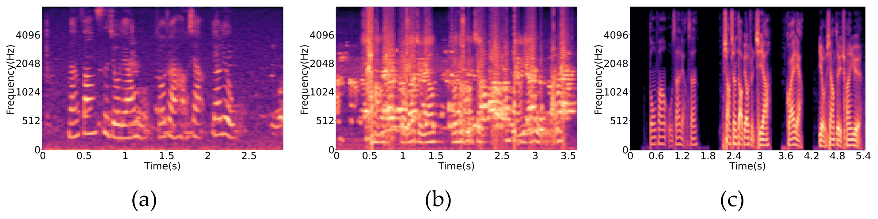
• Inferior speech quality: PCVCs use radio as the transmission vehicle for control command interaction. Generally, the pilot and the controller establish a two-way voice conversation through the transmitter and the receiver in the same designated very high frequency channel. Figure 1a–c shows the Mel spectrogram of several ATC utterances. Clearly, radio signals are inevitably subject to interference, distortion, deformation, and loss during propagation. Consequently, they are vulnerable to noise through direct or indirect coupling, which can result in issues such as degraded reception quality and communication jamming, which adversely affect speech recognition efficiency.
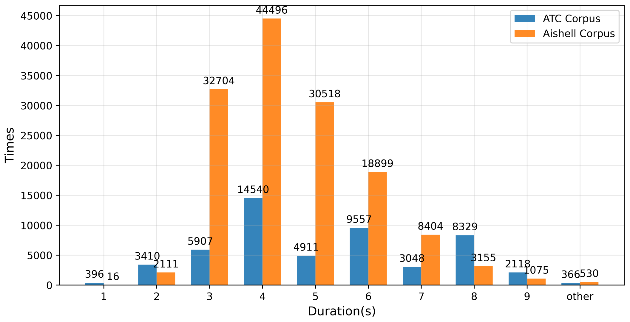
• Excessive speech rate: Since ATC officers have to provide pilots with control instructions, intelligence information, and provision of warning signals in a timely and effective manner, they often have to speak much faster than would occur in normal daily conversation. In busy airspace, with controllers interacting with multiple aircraft simultaneously, the speech rate can be as high as twice the normal rate. This is corroborated by the fact that the average speech rates in the open-source domain training set corpus and the target domain training set corpus we used in this study were 3.16 words/s and 4.75 words/s, respectively. High speech rates and varying accents can adversely affect model decoding.
• Scarcity of calibration data: Most E2E systems require large training sets that have speech data from the appropriate field with text annotations to achieve high accuracy. These training sets could range from hundreds of hours to hundreds of thousands of hours. In addition, the annotation of this large set of speech data requires specialized personnel. As a result, it is a significant challenge to obtain large-scale and high-quality, text-annotated, speech datasets relevant to civil aviation.
• Complications due to partial pronunciation: To avoid the ambiguity of terms leading to the asymmetry of information understanding between the transmitting and receiving ends in PCVCs, the Civil Aviation Administration of China has developed a set of guidelines titled “Radiotelephony Communications for Air Traffic Services”, based on the International Civil Aviation Organization guidelines, to standardize radio communication in China. The Mandarin speech communication standard integrates the control work experience and the daily speech habits. For example, the numbers 1 and 7 have a similar pronunciation. To avoid ambiguity, 1 (yi) is pronounced as yao, and 7 (qi) is pronounced as guai.

In view of the above problems, researchers have carried out various studies. When faced with the small sample problem, and misunderstandings caused by homonyms, or near-homonyms, during PCVCs, Wang et al. proposed a new cross-lingual knowledge transfer learning method and a semi-shared hidden layer cross-lingual DNN architecture in which the number of hidden layers of the source language shared with the target language are tuned and serve as universal transformations [23]. An effective combination of unsupervised pre-training and supervised transfer learning was proposed, where the pre-training is applied to learn speech representations from unlabeled speech samples and the transfer learning is regarded as a subdomain adaption task [24]. A semi-supervised training of a DNN-based AM [25] and a knowledge extraction algorithm [26] were also applied to improve the performance of speech recognition. Zhou et al. suggested the application of a hybrid CTC-attention model to E2E systems in ATC tasks, including the use of CNN networks to improve the encoder architecture to address the noise problem [27]. Multiple CNN kernels, with average pooling operations, were also proposed to address background noise and an unstable speech rate affecting ATC [28].

3. Methodology

3.1. Optimization Measures

Speech recognition has shifted from the structure of multi-modules to an E2E model in recent years. Instead of having separate modules, such as AM (GMM-HMM, DNN-GMM et al.), LM (N-grams, RNNs-based et al.), and PM (phonemes to words), as in the original system, a neural network connects the input (speech waveform or feature sequence) with the output (word or character sequence) and incorporates the functions of the original modules, as shown in Figure 2.

In deep learning research, a long-standing idea is that the final performance depends to a great extent on the data size, coverage and diversity of the training samples. However, the main problem faced by E2E systems is that the scarcity of annotated data in some specific fields leads to serious overfitting problems in classical supervised learning. Therefore, in this study, two approaches, knowledge transfer from auxiliary domains and data augmentation, are proposed to improve the generalization ability of the model on the target task.

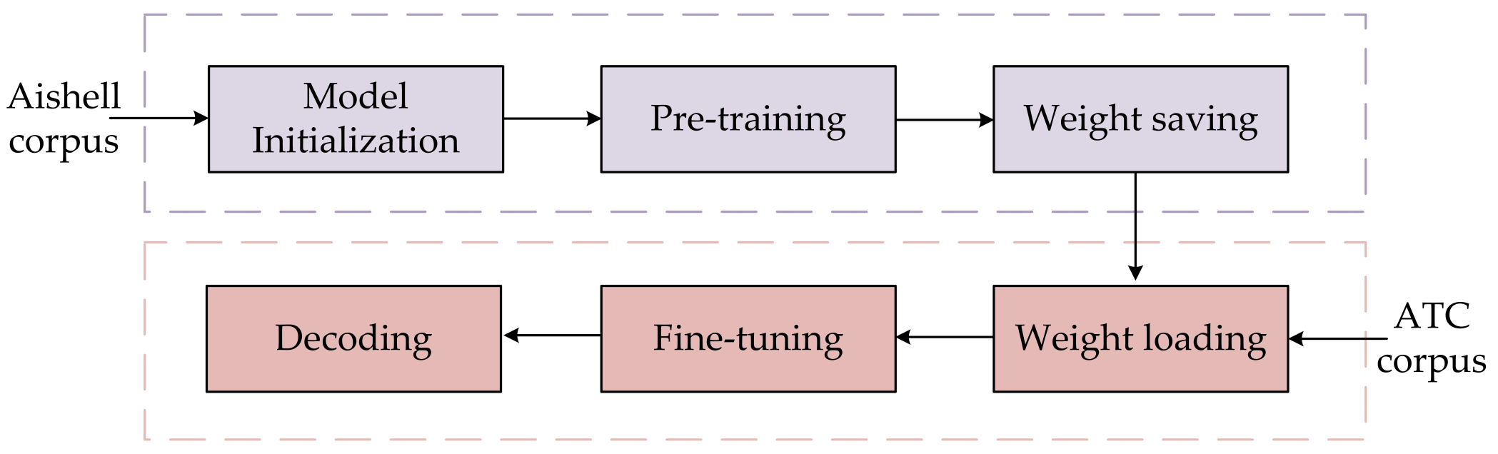
3.1.1. Transfer Learning

Transfer learning from related domains relaxes the constraint encountered in traditional machine learning that training data and test data must have independent and identical distributions. The use of transfer learning makes it possible to mine the invariant essential features and structures of the domain between interrelated domains, thus enabling the transfer and reuse of supervised information, such as annotated data between domains.

The domain consists of two components: the feature space X and its marginal distribution $P\left(x\right)$, where $\{x_1,x_2,\dots ,x_n\}\in X$. Given a domain $D=\{X,P(x\left)\right\}$, the task consists of the label space Y and the target prediction function $f\left(x\right)$. In addition, given a source domain $D_s$, a source domain learning task $T_s$, a target domain $D_t$, and a target domain task $T_t$ (where $D_s$ is not equal to $D_t$, or $T_s$ is not equal to $T_t$), transfer learning uses the knowledge in the source domain $D_s$ and $T_s$ to enhance or optimize the learning efficiency of the target prediction function $f_t\left(x\right)$ in the target domain $D_t$.

As mentioned earlier, transfer learning addresses the scarcity of annotated data in the civil aviation domain and for special pronunciation problems. As shown in Figure 3, we first trained the model on the large-scale source domain Aishell corpus to obtain good transcription capability. Subsequently, we fine-tuned and re-trained the model on the relatively small-scale target domain ATC corpus. Eventually, the model performed well on the source task and retained generalization ability on the target task.

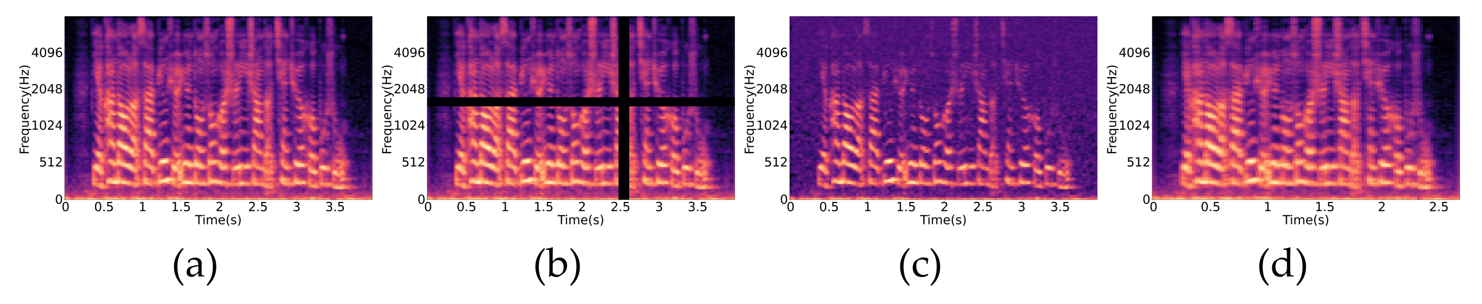
3.1.2. Data Augmentation

Data augmentation is a way to make limited data produce more value equivalent to valid data in the case of the non-substantial addition of extended data. Increasing the sample size and enriching sample diversity by data augmentation can reduce the dependence of the model on certain attributes to improve its generalization ability. However, excessive data augmentation does not lead to the best possible model performance. Optimum model performance can be attained only with an appropriate level of data augmentation.

The source domain that we selected from the Aishell corpus website [29] was recorded in a quiet indoor environment. The recorded text covers eleven fields that include smart home, unmanned vehicle, and industrial production. The basic information of the source domain and target domain datasets were organized and compared, as shown in

Table 1. Basic information of the datasets.

Dataset	Utterances	Total Time (h)	Average Rate (Characters/s)
Aishell corpus	141,600	178	3.16
ATC corpus	50,902	67	4.75

.

The number of samples in the Aishell corpus was approximately three times larger than those in the ATC corpus. Their average speech rates were 3.16 and 4.75 words/s, respectively. Most of the sample durations in the two datasets were between 2 and 8 s, as shown in Figure 4, indicating a nearly consistent sample duration distribution.

Three approaches were used to expand the Aishell corpus in the source domain with reference to the basic features of the two datasets to reduce the variability in the nature of the samples from different domains. Figure 5a shows the Mel spectrogram after visualizing the speech signal of a certain sample in the Aishell corpus. As shown in Figure 5b, the time-frequency masking technique in SpecAugment [30] was used. The maximum range for setting the continuous mask in the temporal (frequency domain) axis direction is 250 ms (100 Hz). In addition, the uniform sampling of one t$\left(f\right)$ is performed in the range $[0,250]$$\left(\right[0,100\left]\right)$, a point $t_0$$\left(f_0\right)$ is randomly selected in the range $[0,\tau -t]$$\left(\right[0,v-f\left]\right)$, and t$\left(f\right)$ successive masks are performed along the time (frequency domain) axis starting from the position $t_0$$\left(f_0\right)$, where $\tau$ and v denote the time dimension and the frequency domain dimension, respectively. In the ATC domain, noise due to the interference of signals from various sources is present in the control speech. Incorporating synthesized Gaussian noise in the source domain data serves as an approximate simulation that is both simple and efficient. Figure 5c displays the Mel spectrogram generated after adding Gaussian white noise with a certain signal-to-noise ratio. As shown in Figure 5d, we performed a $1.5\times$ speed enhancement compared to the average speech rate of both datasets. We refer to this speech data, after the above three changes, as the improved Aishell corpus.

3.2. GAU Module

The MHSA-based transformer fully integrates global information and has powerful parallel computing power, achieving many breakthroughs in natural language processing (NLP) and computer vision fields. However, most transformers are still subjected to short context sizes because of the quadratic complexity of the input length (older information has to be discarded due to the limited memory capacity). GAU, a new transformer variant, still encounters a quadratic complexity problem. However, it has a faster training speed, a lower memory footprint, and better training results than the standard transformer. The core idea behind GAU is to use self-attention and GLU as a unified layer and share as much of their computation as possible. This not only achieves higher computational efficiency, but also naturally empowers a powerful attention-gating mechanism. Currently, GAU has achieved remarkable success in NLP tasks. Therefore, we explored the applicability of GAU in the speech recognition domain in this study, with the structure shown in Figure 6.

The input features first go through layer normalization to ensure the stability of the distribution of each sample feature and to improve the speed of convergence of the model training process. After this, the input features go through the dense layer and are subjected to a non-linear transformation to obtain the gated matrix U, and $Value$, $Query$ and $Key$ of the computing attention scoring, respectively.

$$U={\varphi }_u\left(X{W}_u\right),V={\varphi }_v\left(X{W}_v\right)\in {\mathbb{R}}^{T\times e}$$

(1)

$$Q\&K={\varphi }_{q\&k}\left(X{W}_{q\&k}\right)\in {\mathbb{R}}^{T\times s}$$

(2)

where X ∈ ${\mathbb{R}}^{T\times e}$, T denotes the sequence length, e denotes the expanded intermediate size, s denotes the head size, and $\varphi$ denotes the activation function. Subsequently, the attention score is computed with the $ReL{U}^2$ activation function [31] including the relative position bias [32]. This ensures feature sparsity to some extent and increases the bias in the attention mapping. In addition, the gating mechanism alleviates the burden of attention, which allows the use of a single head attention with almost no quality loss.

$$A=ReL{U}^2(Q{K}^T+B)\in {\mathbb{R}}^{T\times T}$$

(3)

$$O=(U\odot AV)W_0\in {\mathbb{R}}^{T\times d}$$

(4)

where A is the attention matrix to fuse information between tokens and ⊙ denotes element-wise multiplication. Therefore, the output O contains the interactions between tokens. Finally, the use of a dropout layer helps to avoid overfitting during the model training process.

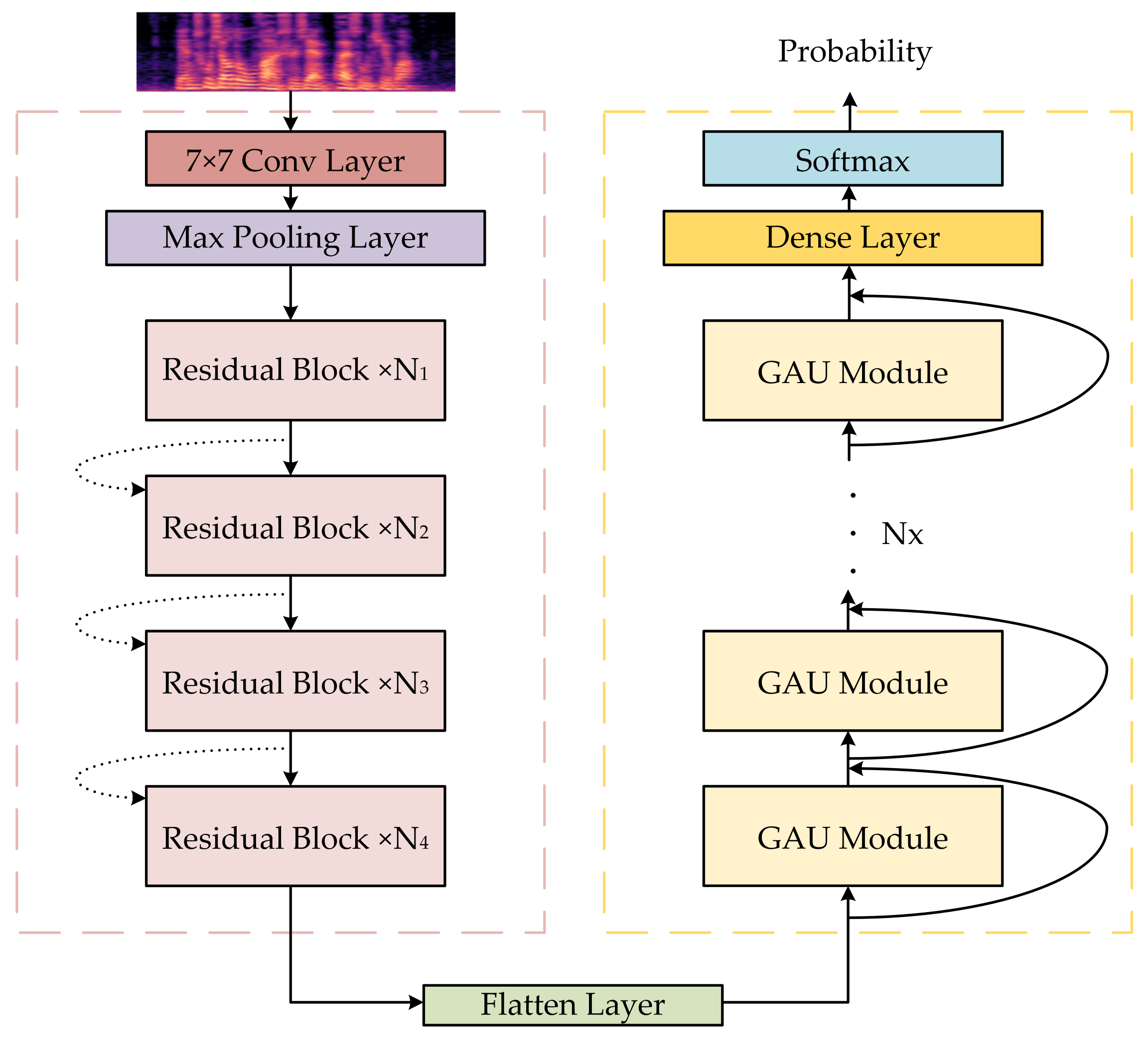
3.3. Overall Architecture of the Model

The Mel spectrogram, as one of the visualization methods of speech signals, contains both time and frequency domain information. We take it as the input of the model. The structure of our model consists of two parts, as shown in Figure 7.

Since CNNs can provide temporal and spatial translation-invariant convolution, we can apply them to the acoustic modeling. Furthermore, the invariance of the convolution is used to realize local information fusion and dimension compression of time series. Therefore, the first part consists of ResNet. When the input goes through the $7\times 7$ conv layer, the convolution kernel first regularly sweeps through the input features, performs matrix element multiplication summation on the input features within the receptive field, and superimposes the bias. Next, the output feature map is passed to the max pooling layer for feature selection and information filtering. Since the pooling layer contains pre-defined pooling functions, we replace the results of the individual points in the feature map with the feature map statistics of their neighboring regions. Finally, the pooled feature vectors pass through a heap consisting of different numbers of residual blocks (Figure 8) sequentially to obtain the highly featured representations with local information interaction, where residual connections are introduced within the blocks and between the heaps. Subsequently, the input is passed across layers and the result of convolution is added to it to alleviate the vanishing gradient problem caused by increasing depth in CNN. Finally, the outputs that have built local temporal-frequential correlations are passed to the flatten layer for dimension reduction to serve as the input for the next part.

The second part is primarily composed of several GAU modules in series. This attention-mechanism-based module solves the problem that RNNs cannot be computed in parallel. However, it cannot capture the word order information. Therefore, we add absolute position coding to the input to ensure consistency in the temporal dimension. Similarly, we connect the residuals between modules to prevent the stacked modules capturing global information among the feature vectors from leading to vanishing gradient and network degradation problems. Finally, the output is passed to the dense layer for linear variation, to map the feature dimension into the classification number in each time step, and passed through the softmax layer to calculate the final classification prediction probability.

3.4. Training and Decoding

The introduction of CTC in the training process eliminates the difficulty of alignment due to differing lengths of input and output sequences in the speech recognition domain. In addition, the introduction of the special character, $blank$ enables each frame of the speech sequence to predict the conditional probability distribution of the corresponding output label sequence in a one-to-one manner. In a given input sequence X $(x_1,x_2,\cdots ,x_T)$ of length T, where $V^{\prime }$ denotes the dictionary $(V^{\prime }=characters\cup \left\{blank\right\})$, the output vectors $y_t$ are normalised with the softmax function, then interpreted as the probability of emitting the label (or $blank$) with index k at time t.

$$P_r(k,t|x)=\frac{exp\left(y_t^k\right)}{{\sum }_{k}exp\left(y_t^k\right)}$$

(5)

where $y_t^k$ represents element k of $y_t$. For a given input sequence X, the conditional probability of any path a in $V^{\prime T}$ is calculated as follows:

$$P_r\left(a\right|x)=\prod _{t=1}^T{P}_r(k,t|x)$$

(6)

where $V^{\prime T}$ denotes the set of all paths of length T defined on $V^{\prime }$. The lengths of the input speech sequence and the output path are equal in the calculation of the path probability. This is primarily ensured by inserting blanks between the outputs and by generating duplicate tokens. The actual speech sequence length is much larger than that of the label, resulting in a multiple-input to single-output mapping. To obtain the predicted sequence, path aggregation (merging identical consecutive tokens and removal of blanks from paths) is performed, followed by the summation of all path probabilities.

$$P_r\left(y\right|x)=\sum _{a\in {\beta }^{-1}\left(y\right)}{P}_r\left(a\right|x)$$

(7)

where $\beta$ is an operator that first removes the repeated labels, then the blanks from alignments and ${\beta }^{-1}\left(y\right)$ denotes all paths corresponding to the label sequences in the set $V^{\prime T}$. The final objective function of CTC is the sum of the negative log probability of all tokens. Thus, the loss can be calculated using a backward–forward algorithm and minimized by back-propagating to train the network.

$$CTC\left(x\right)=-log{P}_r\left(y\right|x)$$

(8)

The decoding process uses a beam search rather than the traditional greedy algorithm [33]. As shown in Figure 9, the search tree is built using a breadth-first strategy and the nodes at each layer of the tree are sorted according to the heuristic cost. After this, only a pre-determined number of nodes are left. These nodes continue to expand at the subsequent layer while the other nodes are clipped. The beam width can either be pre-determined or variable. The search can be performed using a pre-determined minimum cluster width. In case no suitable solution is found, the search can be repeated using an expanded beam width. Finally, the difference between the search solution and the standard solution is evaluated using the Levenshtein distance formula.

4. Experiments

4.1. Experimental Data

The source domain dataset consists of the Aishell corpus and the improved Aishell corpus (hereafter referred to as the expanded Aishell corpus). The training, validation, and test sets contain 240,196, 28,652, and 14,352 speech items, respectively. The ATC corpus is derived from the first-line control recordings of the North China Air Traffic Control Bureau of civil aviation of China, and the control simulation training recordings of the Civil Aviation Flight University of China, with training, validation, and test sets containing 47,084, 2545 and 1273 speech items, respectively. In addition, the modeling unit contains 4243 Chinese characters, one special character, “blank”, and one unknown character, “unk”.

4.2. Experimental Platform

The experiments were performed on a Windows operating system. The computer configuration was as follows: Intel Xeon Silver 4110 CPU, two NVIDIA RTX2080Ti 11 G discrete graphics cards, 128 GB 2 666 MHz ECC memory, 480 GB SSD and a 4 TB SATA hard disk. The Pytorch framework was used to build the neural network model.

4.3. Experimental Analysis

The input used in this study was a Mel spectrogram with shape equal to $(None,$$3, 64, 512)$, where the “None ” is variable. The four dimensions denote batch size, channel, height, and width, respectively. In the training phase, the CTC objective function loss was calculated using the forward–backward algorithm. The model weights were updated using the Adam optimizer [34] with initial learning rate set to $0.0001$ and hyperparameters ${\beta }_1$=$0.9$, ${\beta }_2$=$0.98$, and $ϵ$ = ${10}^{-9}$. A beam search method with a width of 5 was used in the inference process to obtain the final prediction text. In addition, with the same convolutional structure, we selected several representative networks, such as LSTM, GRU, and a transformer variant (MHSA+GLU), to compare the experimental results with our proposed outcomes in the expanded Aishell corpus. In the ATC corpus, the experimental results were analyzed by changing the number of layers of the GAU module and by using different convolutional structures. In these experiments, the final performance on the speech recognition task was evaluated in terms of CER, real-time factor (RTF), total number of parameters, running total time, and training time each step. The CER was calculated according to the following rule:

$$CER=\frac{I+D+S}{N}\times 100\%$$

(9)

where the denominator N represents the total length of the true label and the notation I, D, S denote the number of the insertion, deletion, and substitution operations, respectively. The RTF was applied to evaluate the decoding efficiency.

$$RTF=\frac{T_d}{T_s}$$

(10)

here, $T_s$ is the time decoded for a speech with a duration of $T_d$.

4.3.1. Pre-Training Results of Different Models in the Expanded Aishell Corpus

Our model architecture was based on ResNet34_GAU@24 in the pre-training process. The specific parameter setup is shown in

Table 2. Details of architecture. (input: Mel spectrogram with shape equal to $(None,3,64,512)$).

Structural Order	Output Size	Parameters Setup
Conv layer	$(None,64,32,256)$	$k=(7,7),s=(2,2),f=64$
Max pooling layer	$(None,64,16,128)$	$k=(3,3),s=(2,2)$
Residual block $\times 3$	$(None,64,16,128)$	$\{k_1,k_2=(3,3)$ and $f_1,f_2=64\}\times 3$
Residual block $\times 4$	$(None,128,8,128)$	$\{k_1,k_2=(3,3)$ and $f_1,f_2=128\}\times 4$
Residual block $\times 6$	$(None,256,4,128)$	$\{k_1,k_2=(3,3)$ and $f_1,f_2=256\}\times 6$
Residual block $\times 3$	$(None,512,1,128)$	$\{k_1,k_2=(3,3)$ and $f_1,f_2=512\}\times 3$
Permute	$(None,1,128,512)$	$(0,2,3,1)$
Flatten layer	$(None,128,512)$	$start\_dim=1,end\_dim=2$
GAU module $\times 24$	$(None,128,512)$	$Linear1(512,1024)$ for U, $Linear2(512,1024)$ for V, $Linear3(512,128)$ for $Q\&K$, $Linear4(1024,512)$ for O
Dense layer	$(None,128,4245)$	$Linear(512,len(dict.\left)\right)$

. In the control model, the number of layers of MHSA+GLU was set to be the same as in our framework and we employed eight parallel attention layers, each with a dimension of 64 [15]. In addition, there were four stacked layers each of bidirectional-LSTM (BiLSTM) and bidirectional-GRU (BiGRU), and 512 hidden units per layer, where the trainable parameters were approximately two-thirds of our proposed parameters.

The specific training process loss curve is shown in Figure 10. The number of iteration rounds was 20 epochs (74,980 steps in total), with each step containing 64 samples. During the first 9000 steps, BiLSTM had a significantly slow convergence rate. Although BiGRU and MHSA+GLU had similar convergence rates, the loss curve of GAU had a larger slope and decreased faster after 1000 steps. Thus, GAU had significantly faster convergence than the other three models. During the last 9000 steps, BiLSTM and BiGRU had similar convergence patterns, with a larger range of training loss fluctuations. In contrast, the loss curve amplitudes for MHSA+GLU and GAU were smaller.

The three models were validated and tested after each training epoch. BiLSTM and BiGRU had the lowest CERs of 15.4% and 15.7%, and 17.6% and 17.4%, as shown in in Figure 11a,b, respectively. In comparison, MHSA+GLU and GAU achieved the lowest CERs of 11.0% and 10.2%, and 12.5% and 11.1%, respectively. Our model reduced CERs by 34.4% in the validation set, relative to the RNN-based model, and by 7.3% relative to the multi-head attention-based model. In the test set, the corresponding relative reduction amplitudes were 36.6% and 11.2%.

The comparison of the four models in terms of CER, RTF, total number of parameters, running time, and training time is shown in

Table 3. Evaluation metrics of different models.

Model	CER (%)		RTF	Params	Run Time	Training Time
	dev	Test
ResNet34_BiLSTM@4	15.4	17.6	0.24	46.9 M	15.7 h	1.51 s/step
ResNet34_BiGRU@4	15.7	17.4	0.23	41.2 M	14.2 h	1.36 s/step
ResNet34_MHSA-GLU@24	11.0	12.5	0.20	93.2 M	13.9 h	1.33 s/step
ResNet34_GAU@24 (ours)	10.2	11.1	0.18	63.3 M	12.7 h	1.22 s/step

. The total number of parameters of our model was 63.3 M, which was 1.35, 1.54, and 0.68 times higher than those of BiLSTM, BiGRU, and MHSA+GLU, respectively. In addition, our model was more competitive in recognition results, as compared to other models, with less time taken per step and total time needed for the training process. The average RTFs for the test samples were 0.24, 0.23, 0.20, and 0.18, respectively, which means that the time consumption of the proposed approach for decoding a 10-s speech was approximately 1.8 s.

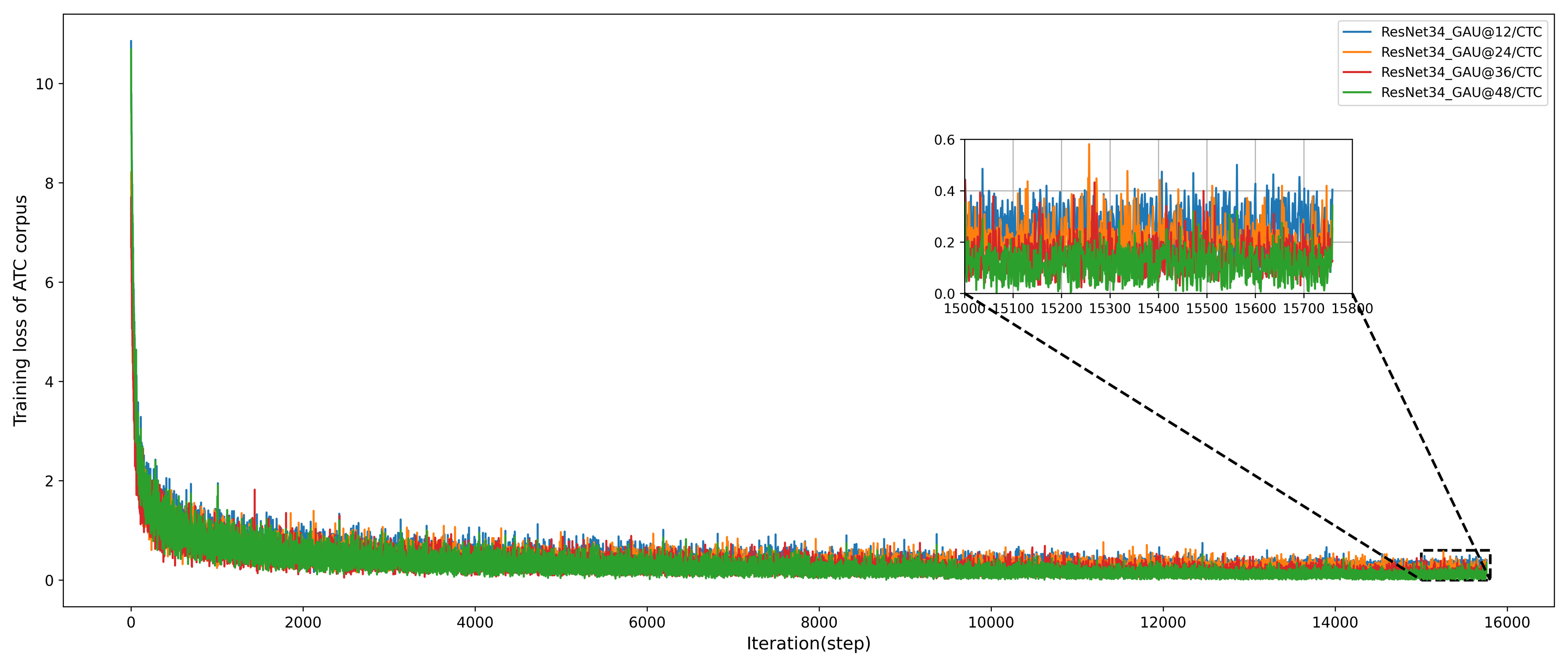
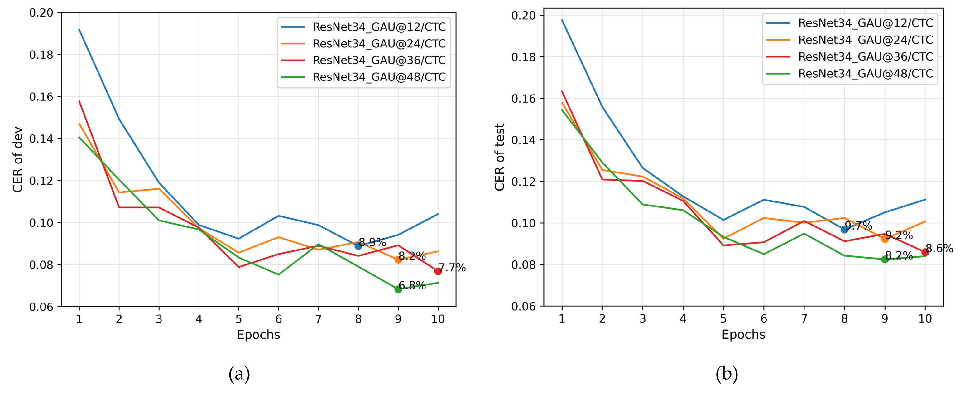
4.3.2. Experimental Results of GAU Module with Different Number of Layers in the ATC Corpus

Our model achieved satisfactory results on the source task. To explore the effect of layer changes on the final recognition results of the target task, we used the optimal weights of GAU modules with different layers during the expanded Aishell corpus test as the initialization parameters for training on the ATC corpus dataset. The training process is shown in Figure 12. There were ten epochs (15,760 steps in total), with 64 samples in each step. GAU modules with 12, 24, 36, and 48 layers all attained a fast convergence rate. From 15,000 steps to the end of the iteration, the convergence rate was more stable as the number of layers increased.

Figure 13a,b show a comparison of the CERs of GAU modules with different layers on the ATC corpus validation, and on the test set. After one epoch of iteration, the CER of the 12-layer GAU module was approximately 19% and 20%, while the CERs of the 24-, 36- and 48-layer GAU modules were all approximately 15% and 16%. As the number of iteration epochs increased, the lowest CERs for the 12-, 24-, 36-, and 48-layer GAU modules were 8.9%, 8.2%, 7.7%, and 6.8%, as well as 9.7%, 9.2%, 8.6%, and 8.2%, respectively. Furthermore, the CERs of the 48-layer GAU module were lower than those of the 12-layer GAU module by 23.6% and 15.5%, respectively.

As shown in

Table 4. Evaluation metrics of GAU module with different layers in the ATC corpus.

Model	CER (%)		RTF	Params	Run Time	Training Time
	dev	Test
ResNet34_GAU@12	8.9	9.7	0.16	43.6 M	1.6 h	0.74 s/step
ResNet34_GAU@24	8.2	9.2	0.18	63.3 M	2.3 h	1.03 s/step
ResNet34_GAU@36	7.7	8.6	0.21	83.0 M	3.0 h	1.36 s/step
ResNet34_GAU@48	6.8	8.2	0.23	102.7 M	3.9 h	1.76 s/step

, the training time increased linearly with an increase in the number of layers and the total number of parameters of the model. This increase in the number of GAU modules connected by residuals led to a significant improvement in recognition accuracy.

4.3.3. Experimental Results of Different Convolutional Architectures in the ATC Corpus

The effects of different convolutional structures on the experimental results of the target task are shown in

Table 5. Evaluation metrics of different convolutional architectures in the ATC corpus.

Model	CER (%)		RTF	Params	Run Time	Training Time
	dev	Test
VGG16_GAU@48	7.1	8.3	0.23	102.4 M	4.1 h	1.88 s/step
VGG19_GAU@48	6.9	8.2	0.25	107.8 M	5.0 h	2.31 s/step
ResNet34_GAU@48	6.8	8.2	0.23	102.7 M	3.9 h	1.76 s/step
ResNet50_GAU@48	6.8	8.0	0.24	106.0 M	4.4 h	2.01 s/step

. To ensure the approximate number of total parameters, we set the number of layers of the GAU module as 48 and selected VGG16, VGG19, ResNet34, and ResNet50 as the experimental controls. No significant difference was observed in the training time spent by each network architecture. The step durations for the four models were 1.88 s, 2.31 s, 1.76 s, and 2.01 s, respectively, and the total training time was kept within 5 h. The CERs of the four models on the validation and test sets were 7.1%, 6.9%, 6.8%, and 6.8%, as well as 8.3%, 8.2%, 8.2%, and 8.0%, respectively. Although the ResNet-based model slightly outperformed the VGG architecture [35], the different convolutional architectures did not improve the final recognition rate significantly.

5. Conclusions

In this study, a new E2E speech recognition model ResNet–GAU–CTC was developed. Specifically, ResNet extracts the time-frequency domain features of speech signals, the GAU module captures the global interaction information between sequences, and CTC automatically aligns the input and output sequences that may be unequal in length. In addition, this study proposes transfer learning and data augmentation technologies to solve the challenges faced by ATC-related Mandarin speech recognition. The former technology addresses the problems of scarcity of ATC domain-related annotated data and special pronunciation of certain phrases, whereas the latter expands the source domain data, enriches the diversity of data features, reduces the variability of data distribution among different domains, and improves the generalization ability of the model after transfer learning. The CER of the model on the source task was 11.1%. Furthermore, ResNet50_GAU@48 achieved optimal recognition performance and the CER decreased to 8.0% on the target task. We will collect and expand the ATC corpus to optimize our model in future work. In addition, we aim to address the control speech recognition tasks in English and mixed Mandarin–English scenarios to provide technical support for the application of ASR in the ATC field.

References

1. Juang, B.H.; Rabiner, L.R. Hidden Markov Models for speech recognition. Technometrics 2012, 33, 251–272. [Google Scholar] [CrossRef]
2. Zweig, G.; Russell, S. Speech recognition with Dynamic Bayesian Networks. In Proceedings of the AAAI-98: Fifteenth National Conference on Artificial Intelligence, Madison, WI, USA, 26–30 July 1998. [Google Scholar]
3. Liu, X.; Gales, M. Automatic model complexity control using marginalized discriminative growth functions. IEEE Workshop Autom. Speech Recognit. Underst. 2007, 15, 1414–1424. [Google Scholar] [CrossRef]
4. Abe, A.; Kazumasa, Y.; Seiichi, N. Robust speech recognition using DNN-HMM acoustic model combining noise-aware training with spectral subtraction. In Proceedings of the 16th Annual Conference of the International-Speech-Communication-Association (INTERSPEECH 2015), Dresden, Germany, 10 June 2015. [Google Scholar]
5. Hinton, G.; Deng, L.; Yu, D.; Dahl, G.E.; Kingsbury, B. Deep Neural Networks for Acoustic Modeling in Speech Recognition: The Shared Views of Four Research Groups. IEEE Signal Process. Mag. 2012, 29, 82–97. [Google Scholar] [CrossRef]
6. Mohamed, A.; Dahl, G.E.; Hinton, G. Acoustic modeling using Deep Belief Networks. IEEE Trans. Audio Speech Lang. Process. 2011, 20, 14–22. [Google Scholar] [CrossRef]
7. Graves, A.; Fernandez, S.; Gomez, F.; Schmidhuber, J. Connectionist temporal classification: Labelling unsegmented sequence data with recurrent neural networks. In Proceedings of the 23rd International Conference on Machine Learning (ICML’06), New York, NY, USA, 25 June 2006. [Google Scholar]
8. Graves, A.; Jaitly, N. Towards end-to-end speech recognition with recurrent neural networks. In Proceedings of the International Conference on Machine Learning, Bejing, China, 22–24 June 2014. [Google Scholar]
9. Hochreiter, S.; Schmidhuber, J. Long short-term memory. Neural Comput. 1997, 9, 1735–1780. [Google Scholar] [CrossRef] [PubMed]
10. Chung, J.; Gulcehre, C.; Cho, K.H.; Bengio, Y. Empirical Evaluation of Gated Recurrent Neural Networks on Sequence Modeling. arXiv 2014, arXiv:1412.3555. [Google Scholar]
11. Zhang, Y.; Lu, X. A speech recognition acoustic model based on LSTM -CTC. In Proceedings of the 2018 IEEE 18th International Conference on Communication Technology (ICCT), Chongqing, China, 1 October 2018. [Google Scholar]
12. Shi, Y.Y.; Hwang, M.-Y.; Liu, X. End-To-End speech recognition using a high rank LSTM-CTC based model. In Proceedings of the IEEE International Conference on Acoustics, Speech and Signal Processing (ICASSP), Brighton, UK, 12 March 2019. [Google Scholar]
13. Amodei, D.; Ananthanarayanan, S.; Anubhai, R.; Bai, J.; Zhu, Z. Deep Speech 2: End-to-End Speech Recognition in English and Mandarin. In Proceedings of the 33rd International Conference on Machine Learning, New York, NY, USA, 20–22 June 2016. [Google Scholar]
14. Wang, D.; Wang, X.D.; Lv, S.H. End-to-end mandarin speech recognition combining CNN and BLSTM. Symmetry 2019, 11, 644. [Google Scholar] [CrossRef]
15. Vaswani, A.; Shazeer, N.; Parmar, N.; Uszkoreit, J.; Jones, L.; Gomez, A.N.; Kaiser, L.; Polosukhin, I. Attention Is All You Need. In Proceedings of the 31st Annual Conference on Neural Information Processing Systems (NIPS), Long Beach, CA, USA, 4–9 December 2017. [Google Scholar]
16. Zhang, Q.; Lu, H.; Sak, H.; Tripathi, A.; McDermott, E.; Koo, S.; Kumar, S. Transformer Transducer: A streamable speech recognition model with transformer encoders and RNN-T loss. In Proceedings of the IEEE International Conference on Acoustics, Speech and Signal Processing (ICASSP), Barcelona, Spain, 8 April 2020. [Google Scholar]
17. Shazeer, N. GLU Variants Improve Transformer. arXiv 2020, arXiv:2002.05202. [Google Scholar]
18. Du, N.; Huang, Y.P.; Andrew, M.D. GLaM: Efficient Scaling of Language Models with Mixture-of-Experts. arXiv 2021, arXiv:2112.06905. [Google Scholar]
19. Romal, T.; Daniel, D.F.; Jamie, H. Lamda: Language Models for Dialog Applications. arXiv 2022, arXiv:2201.08239. [Google Scholar]
20. He, K.M.; Zhang, X.Y.; Ren, S.Q.; Sun, J. Deep residual learning for image recognition. In Proceedings of the IEEE Conference on Computer Vision and Pattern Recognition (CVPR), Las Vegas, NV, USA, 30 June 2016. [Google Scholar]
21. Hua, W.; Dai, Z.; Liu, H.; Le, Q.V. Transformer Quality in Linear Time. arXiv 2022, arXiv:2202.10447. [Google Scholar]
22. Holone, H. Possibilities, Challenges and the State of the Art of Automatic Speech Recognition in Air Traffic Control. Int. J. Comput. Inf. Eng. 2015, 9, 1933–1942. [Google Scholar]
23. Wang, J.; Liu, S.H.; Yang, Q. Transfer learning for air traffic control LVCSR system. In Proceedings of the 2017 Second International Conference on Mechanical, Control and Computer Engineering (ICMCCE), Harbin, China, 10 December 2017. [Google Scholar]
24. Lin, Y.; Li, Q.; Yang, B. Improving speech recognition models with small samples for air traffic control systems. Neurocomputing 2021, 445, 287–297. [Google Scholar] [CrossRef]
25. Midl, L.; Vec, J.; Praak, A.; Trmal, J. Semi-supervised training of DNN-based acoustic model for ATC speech recognition. In Proceedings of the 20th International Conference, SPECOM 2018, Leipzig, Germany, 18–22 September 2018. [Google Scholar]
26. Srinivasamurthy, A.; Motlice, P.; Himawan, I. Semi-supervised learning with semantic knowledge extraction for improved speech recognition in air traffic control. In Proceedings of the Interspeech 2017, Stockholm, Sweden, 20–24 August 2017. [Google Scholar]
27. Zhou, K.; Yang, Q.; Sun, X.S.; Liu, S.H.; Lu, J.J. Improved CTC-Attention Based End-to-End Speech Recognition on Air Traffic Control. In Proceedings of the 9th International Conference on Intelligence Science and Big Data Engineering (IScIDE), Nanjing, China, 17–20 October 2019. [Google Scholar]
28. Lin, Y.; Guo, D.; Zhang, J.; Chen, Z.; Yang, B. A Unified Framework for Multilingual Speech Recognition in Air Traffic Control Systems. IEEE Trans. Neural Netw. Learn. Syst. 2021, 32, 3608–3620. [Google Scholar] [CrossRef] [PubMed]
29. Bu, H.; Du, J.Y.; Na, X.Y.; Wu, B.G.; Zheng, H. AISHELL-1: An open-source Mandarin speech corpus and a speech recognition baseline. In Proceedings of the 20th Conference of the Oriental-Chapter-of-the-International-Coordinating-Committee-on-Speech-Databases-and-Speech-I/O-Systems-and-Assessment (O-COCOSDA), Seoul, Korea, 1–3 November 2017. [Google Scholar]
30. Park, D.S.; Chan, W.; Zhang, Y.; Chiu, C.C.; Zoph, B.; Cubuk, E.D.; Le, Q.V. SpecAugment: A Simple Data Augmentation Method for Automatic Speech Recognition. arXiv 2019, arXiv:1904.08779. [Google Scholar]
31. So, D.R.; Manke, W.; Liu, H.; Dai, Z.; Shazeer, N.; Le, Q.V. Primer: Searching for Efficient Transformers for Language Modeling. arXiv 2021, arXiv:2109.08668. [Google Scholar]
32. Liu, Z.; Lin, Y.; Cao, Y.; Hu, H.; Wei, Y.; Zhang, Z.; Lin, S.; Guo, B. Swin Transformer: Hierarchical Vision Transformer using Shifted Windows. In Proceedings of the IEEE/CVF International Conference on Computer Vision (ICCV), Montreal, QC, Canada, 11–17 October 2021. [Google Scholar]
33. Thomas, H.; Charles, E.; Ronald, L. Introduction to Algorithms, 3rd ed.; The MIT Press: Cambridge, MA, USA, 2009. [Google Scholar]
34. Kingma, D.; Ba, J. Adam: A Method for Stochastic Optimization. arXiv 2014, arXiv:1412.6980. [Google Scholar]
35. Simonyan, K.; Zisserman, A. Very Deep Convolutional Networks for Large-Scale Image Recognition. arXiv 2014, arXiv:1409.1556. [Google Scholar]
Figure 1. (ac) Mel spectrogram of several ATC utterances.
Aerospace 09 00395 g001
Figure 2. Comparison between traditional and E2E speech recognition.
Aerospace 09 00395 g002
Figure 3. Transfer learning between different fields.
Aerospace 09 00395 g003
Figure 4. Duration distribution chart of two datasets.
Aerospace 09 00395 g004
Figure 5. Speech signal visualization of one utterance in the Aishell corpus. (a) Raw Mel spectrogram. (b) Masked Mel spectrogram. (c) Mel spectrogram with Gaussian noise. (d) Mel spectrogram with 1.5× speech rate.
Aerospace 09 00395 g005
Figure 6. GAU Module.
Aerospace 09 00395 g006
Figure 7. Overall framework of the model.
Aerospace 09 00395 g007
Figure 8. Residual block in ResNet with different number of layers. (a) Residual block for ResNet34. (b) Residual block for ResNet50.
Aerospace 09 00395 g008
Figure 9. Beam search with beam width equal to 2.
Aerospace 09 00395 g009
Figure 10. Pre-training loss of different models.
Aerospace 09 00395 g010
Figure 11. Pre-training CER of different models. (a) CER of expanded Aishell corpus for dev. (b) CER of expanded Aishell corpus for test.
Aerospace 09 00395 g011
Figure 12. Training loss of GAU module with different number of layers in the ATC corpus.
Aerospace 09 00395 g012
Figure 13. CERs of GAU modules with different layers in the ATC corpus dataset. (a) CER of ATC corpus for dev. (b) CER of ATC corpus for test.
Aerospace 09 00395 g013