Bivariate-Dependent Reliability Estimation Model Based on Inverse Gaussian Processes and Copulas Fusing Multisource Information

Abstract

Reliability estimation for key components of a mechanical system is of great importance in prognosis and health management in aviation industry. Both degradation data and failure time data contain abundant reliability information from different sources. Considering multiple variable-dependent degradation performance indicators for mechanical components is also an effective approach to improve the accuracy of reliability estimation. This study develops a bivariate-dependent reliability estimation model based on inverse Gaussian process and copulas fusing degradation data and failure time data within one computation framework. The inverse Gaussian process model is used to describe the degradation process of each performance indicator. Copula functions are used to capture the dependent relationship between the two performance indicators. In order to improve the reliability estimation accuracy, both degradation data and failure time data are used simultaneously to estimate the unknown parameters in the degradation model based on the likelihood function transformed using the zeros-ones trick. A simulation study and a real application in the reliability estimation of mechanical seal used in airborne hydraulic pump are conducted to validate the effectiveness and accuracy of the proposed model compared with existing reliability models.

1. Introduction

Accurate reliability estimation for critical components of a mechanical system is crucially important in the aviation industry [1,2]. Reliability information can be obtained from various sources, including degradation data and failure lifetime data [3]. Failure lifetime data represent the reliability information for mechanical component on the time scale. However, sufficient lifetime data are very difficult to obtain only by life testing or even accelerated life testing for those mechanical components with the characteristics of long life and small sample [4]. Degradation data describe the entire degradation process from start to failure [5]. Degradation data can be monitored and collected by sensors. Making full use of available reliability information of mechanical components, including degradation data and failure lifetime data, can improve the accuracy of the reliability estimation and guide optimal maintenance [6].

According to Zhang et al. [7], three main types of reliability estimation models have been developed in recent years, namely knowledge-based, physical-based and data-driven models. A data-driven model is much more flexible to implement and perform the reliability estimation of mechanical components [8]. Regarding degradation data-based models, a stochastic process degradation model is commonly used to build the degradation model of mechanical components, such as the Wiener process, inverse Gaussian (IG) process and Gamma process [9,10,11]. However, uncertainties and discreteness cannot be ignored when using the degradation data to model the degradation process [12,13]. Regarding lifetime data-based models, various statistical distribution [14,15,16] can be used to describe the failure lifetime distribution. However, only enough failure lifetime data can ensure the required prediction accuracy [17], and it is quite hard to obtain sufficient lifetime data for certain high reliability mechanical components even by accelerated life testing. Given that neither of these two types of reliability data can provide a large enough sample to assess reliability, it is reasonable and meaningful to incorporate degradation data and failure lifetime data to support and improve reliability estimation.

Multiple performance indicators can reflect the degradation of mechanical components. Additionally, these performance indicators might be dependent on each other due to the same failure mode or the same working operations. Considering that dependent performance indicators can improve the accuracy of reliability estimation [18,19], the copula function, which is a flexible method to describe the dependent structure, has been widely used in the reliability field [20,21,22]. The copula function can not only be used to establish the joint distribution of multiple variables, but also describe the dependence among the multiple margins. The input marginal distribution for copula function can be degradation data or failure lifetime data. Sun et al. [20] built a multivariate-dependent accelerated degradation model using the nonlinear Wiener process and D-vine copula considering multiple sources of uncertainties. Fang et al. [21] used stochastic processes to describe the degradation process of two performance indicators, using different copula functions to establish the dependent relationship between two indicators, and the Bayesian information criterion (BIC) to choose the best degradation model. Saberzadeh et al. [23] used stochastic models and copula function to build a system reliability model. Andersen et al. [24] presented replacement optimization framework in multi-component systems. The degradation models for components are described by a multivariate gamma process model and the dependent structure is described by Lévy copula. Zhang et al. [25] analyzed two dependent failure modes of solid lubricated bearings and built an accelerated life testing model based on the Weibull distribution and time-varying Frank copula. The deviance information criterion (DIC) is used to determine the best lifetime model.

In order to make full use of multiple sources of reliability information, it is natural to employ a Bayesian method with available data. From a system reliability perspective, Li et al. [26] proposed a Bayesian multi-level information aggregation method to model the system level reliability. Jackson et al. [27] developed a model for the reliability estimation of a multi-state on-demand system with overlapping failure lifetime data. Regarding the reliability model for mechanical components, Wang et al. [28] integrated the field data and accelerated degradation data from the laboratory using calibration factors to predict the reliability of components under the actual field conditions. Pan [29] also used the calibration factor method to construct the link between accelerated life testing data and field failure data. Wang et al. [30] developed a comprehensive model using Bernoulli data, lifetime data and degradation data to improve the accuracy of reliability estimation. Ma et al. [31] used the IG process, taking measurement errors into account, to describe the degradation process, and integrated accelerated lifetime tests (ALT) and accelerated degradation test (ADT) to build a reliability estimation model. Guo et al. [32] integrated both failure lifetime data and degradation data to obtain accurate reliability analysis under Bayesian framework. Guo et al. [33] also built a degradation model based on the Gamma process taking individual heterogeneity into account. Original information about the equipment manufacturers is used as prior information for the degradation analysis of information from the monitoring of the conditions. Wang et al. [34] used accelerated degradation data as prior information. The prior distribution types of random parameters are determined by Anderson–Darling statistic. The reliability model is constructed based on the Wiener process with random effects. Tang et al. [35] proposed a two-step RUL prediction method based on the Wiener process fusing failure lifetime data and field degradation data. These studies aimed to solve the problem of evaluating the reliability of system components or systems. However, most of them only consider degradation or failure time data or consider only one performance indicator or two independent performance indicators. Few of them contribute to the model considering both dependent performance indicators and combining different types of data source.

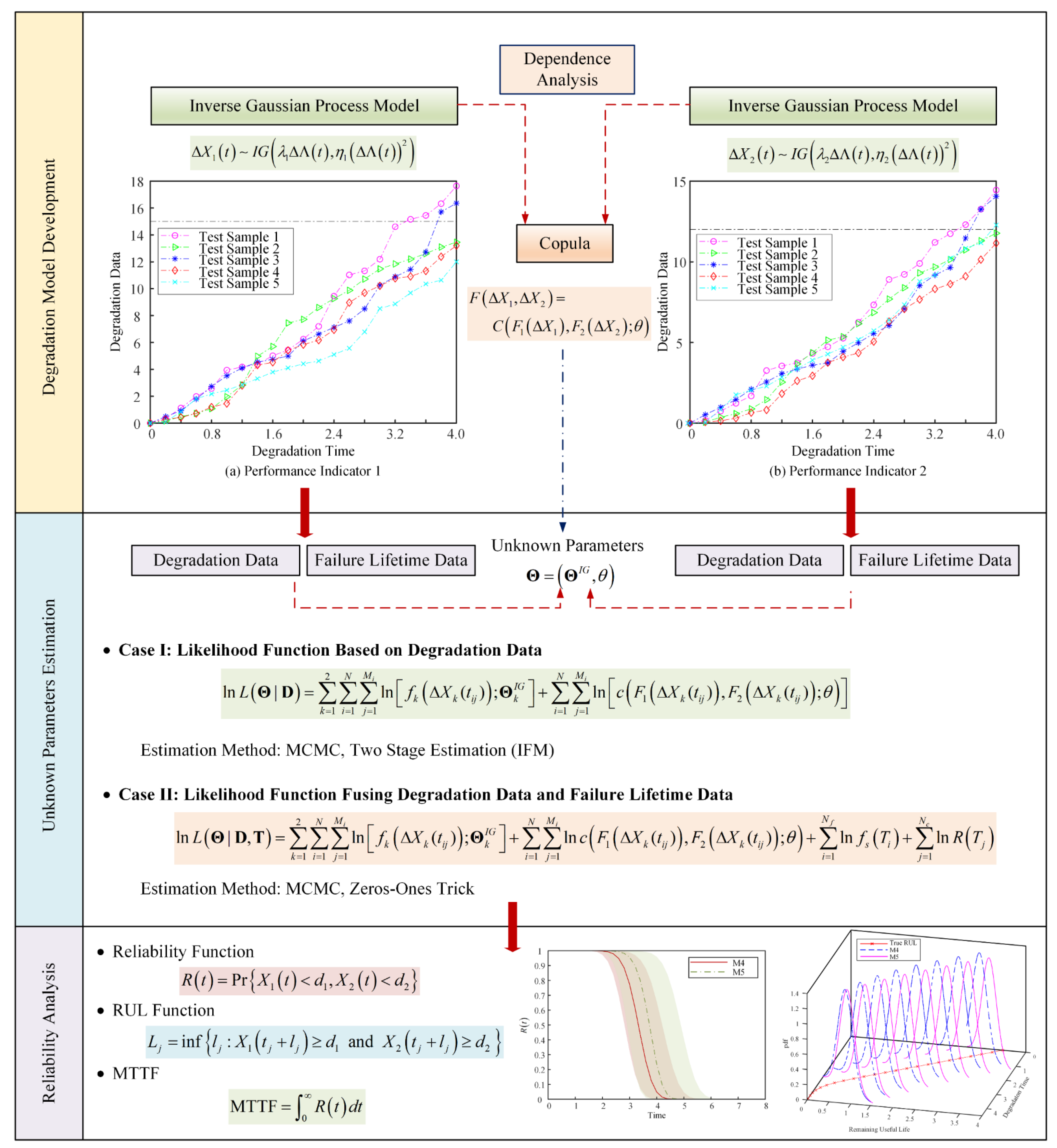
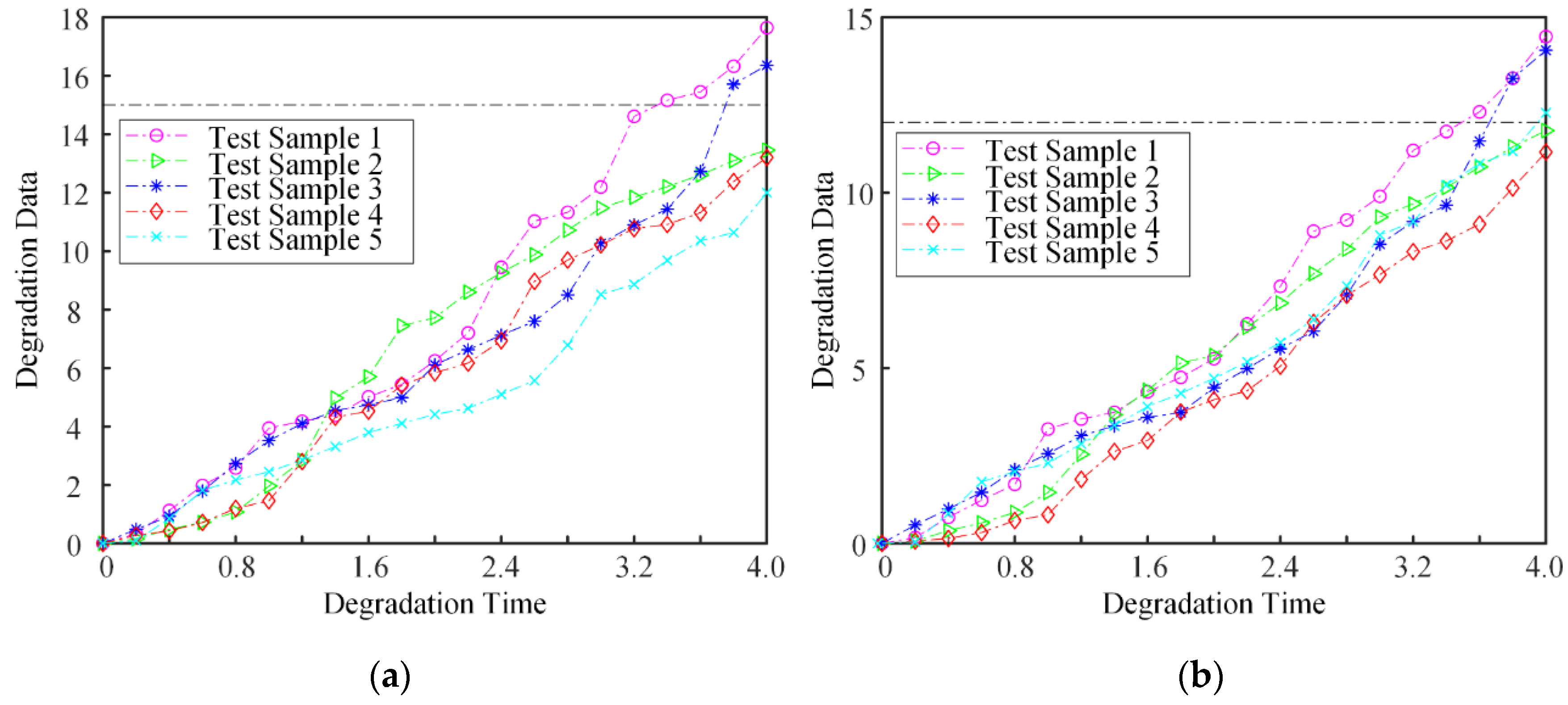
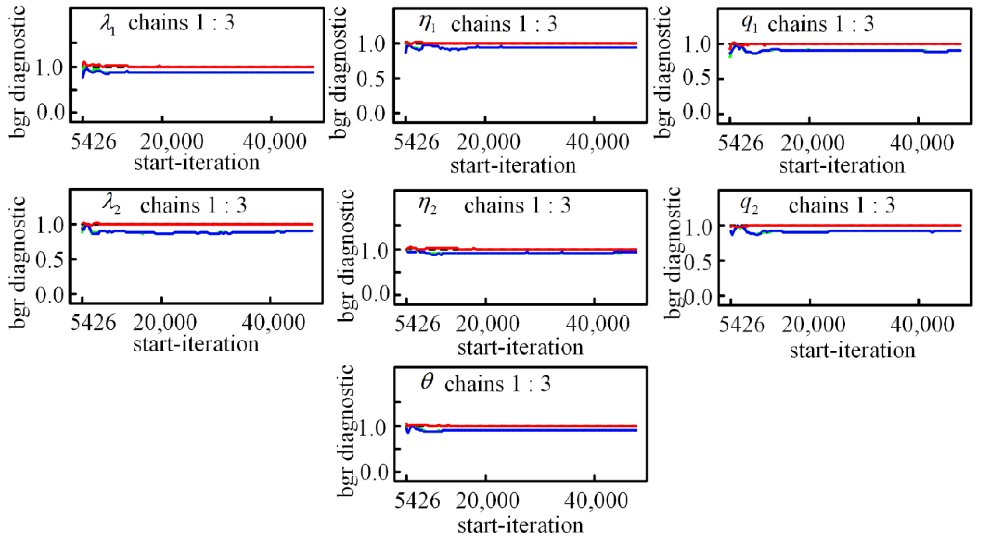
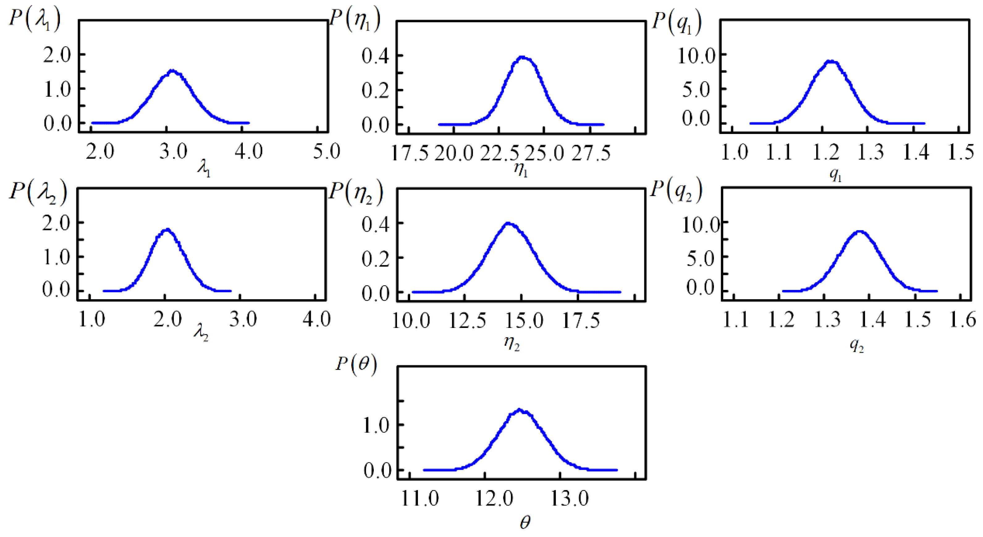
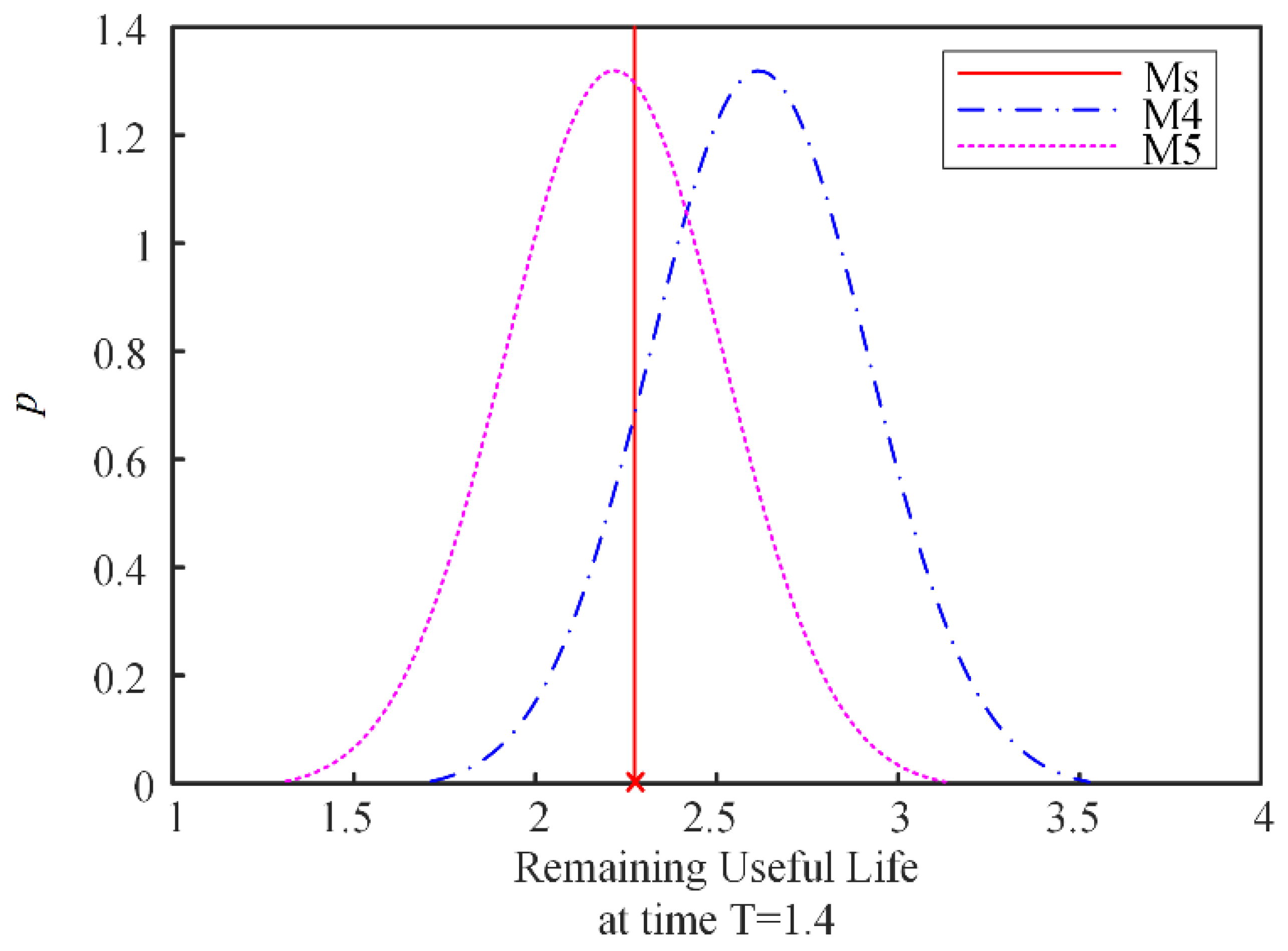
To solve this problem and improve the accuracy of the reliability evaluation and life prediction for lifecycle management, this study develops a reliability evaluation method by integrating likelihood functions with both degradation data and failure lifetime data considering two dependent performance indicators. First, the degradation trajectories of the two performance indicators of the components are both described by the IG process, and copula functions are used to describe the dependency relationship between the two performance indicators. Different from the existing bivariate copula reliability models, both the degradation data and failure lifetime data are integrated in order to improve the accuracy of the reliability estimation and remaining useful life (RUL) prediction. The zeros-ones trick and Bayesian Markov chain Monte Carlo (MCMC) method are used to estimate the unknown parameters. The Akaike information criterion (AIC) and BIC are used to select the best copula function linking two marginal distributions of the two performance indicators. Finally, the reliability estimation and RUL prediction are performed based on the proposed model and it is validated by the simulation study and mechanical seal degradation experiments.

The rest of this paper is organized as follows. In Section 2, the reliability estimation model based on the IG process and copula function is presented. Section 3 shows the likelihood functions built for two cases, where the first one only considers degradation data and the second one considers both degradation data and failure lifetime data. Parameter estimation procedures are performed based on different likelihood functions. In Section 4, a simulation study is described to illustrate the accuracy of the proposed model. 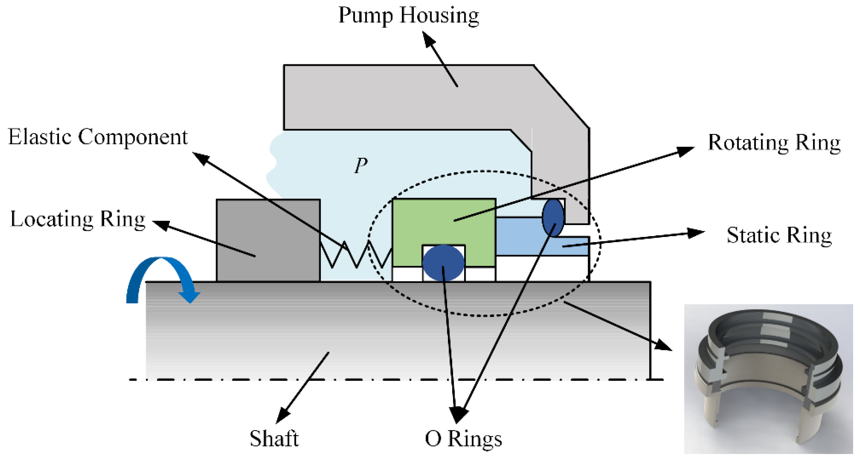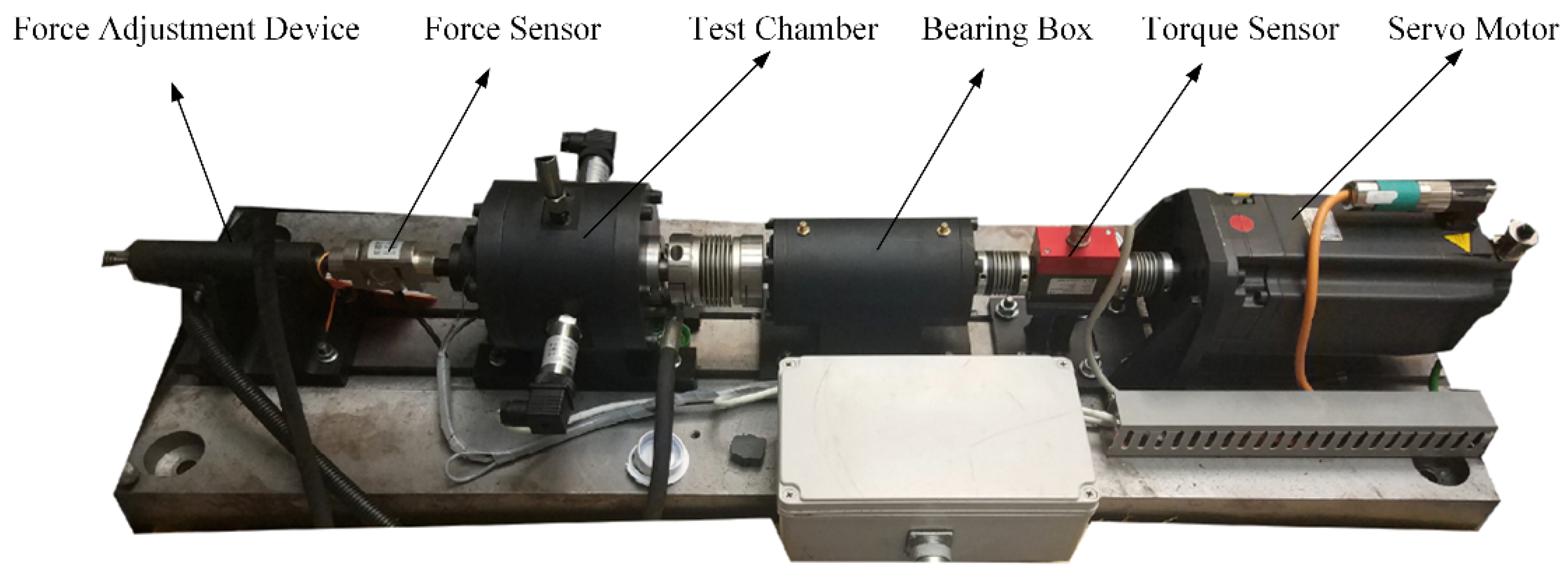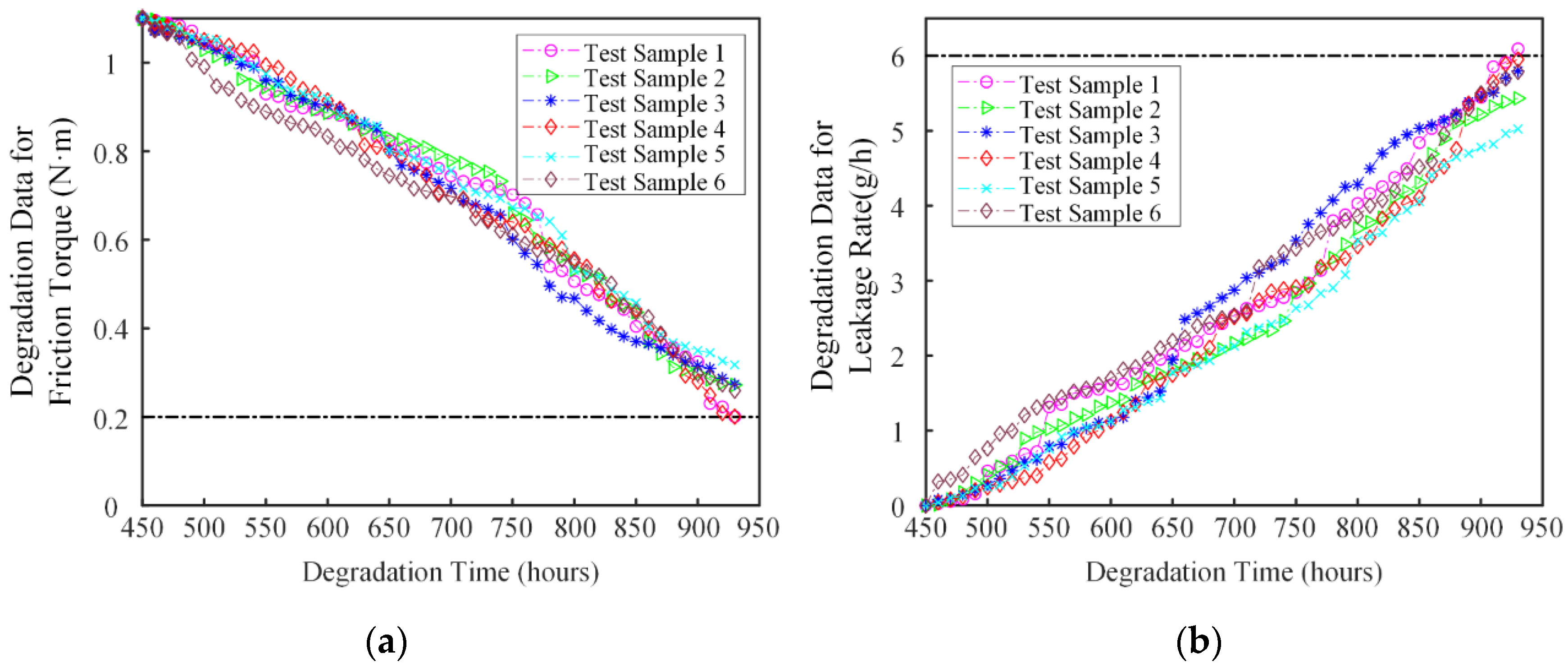In Section 5, the degradation data and failure lifetime data from mechanical seal are used to validate the proposed model. In Section 6, the overall conclusions of this study are summarized.

2. Model Development

2.1. The IG Process Model

IG process is a monotonically increasing process and it has been widely applied in the monotonic degradation process for mechanical components [36,37]. In our study, two degradation performance indicators are assumed to be modeled by the IG process. The IG process $\left\{X\left(t\right),t\ge 0\right\}$ has the following properties:

(1)

the initial value $X\left(0\right)\equiv 0$ with probability one;

(2)

the degradation increments are independent for separate time intervals.

(3)

the degradation increment $\Delta X\left(t\right)=X\left(t+\Delta t\right)-X\left(t\right)$ follows the IG distribution:

$$\Delta X\left(t\right)\sim IG\left(\lambda \Delta \mathsf{\Lambda }\left(t\right),\eta {\left(\Delta \mathsf{\Lambda }\left(t\right)\right)}^2\right)$$

(1)

where $\lambda ,\eta >0$, $\mathsf{\Lambda }\left(t\right)$ is the monotonic time scale function representing the degradation trajectory, and $\Delta \mathsf{\Lambda }\left(t\right)=\mathsf{\Lambda }\left(t+\Delta t\right)-\mathsf{\Lambda }\left(t\right)$. It can be expressed as a power-law function, exponential function, obtained by the failure mechanism model or fitted by the degradation data [38,39]. In particular, $\mathsf{\Lambda }\left(t\right)=t^q$ is commonly used. When $q=1$, it means the degradation trajectory is linear. When $q>1$, it means that the degradation trajectory is concave. When $q<1$, it means that the degradation trajectory is convex. Since $\mathsf{\Lambda }\left(t\right)=t^q$ can describe different types of degradation paths, we will adopt it without the loss of generality.

The cumulative distribution function (CDF) and probability destination function (PDF) of $\Delta X\left(t\right)$. $\Delta X\left(t\right)$ can be obtained by:

$$F\left(\Delta X\left(t\right)\right)=\mathsf{\Phi }\left(\sqrt{\frac{\eta {\left(\Delta \mathsf{\Lambda }\left(t\right)\right)}^2}{\Delta X\left(t\right)}}\left(\frac{\Delta X\left(t\right)}{\lambda \Delta \mathsf{\Lambda }(t)}-1\right)\right)+\exp \left(\frac{2\eta }{\lambda }\Delta \mathsf{\Lambda }(t)\right)\mathsf{\Phi }\left(-\sqrt{\frac{\eta {\left(\Delta \mathsf{\Lambda }\left(t\right)\right)}^2}{\Delta X\left(t\right)}}\left(\frac{\Delta X\left(t\right)}{\lambda \Delta \mathsf{\Lambda }(t)}+1\right)\right)$$

(2)

$$f\left(\Delta X(t)\right)=\sqrt{\frac{\eta {\left(\Delta \mathsf{\Lambda }\left(t\right)\right)}^2}{2\pi {\left(\Delta X(t)\right)}^3}}\exp \left\{-\frac{\eta {\left(\Delta X(t)-\lambda \Delta \mathsf{\Lambda }(t)\right)}^2}{2{\lambda }^2\Delta X(t)}\right\}$$

(3)

where $\mathsf{\Phi }(\cdot )$ is the standard normal CDF.

The failure time $T$ denotes the time at which the degradation path first reaches a predefined threshold $d$, and it can be expressed as:

$$T=\inf \left\{t:X\left(t\right)>d\right\}$$

(4)

Considering that $X\left(t\right)~IG\left(\lambda \mathsf{\Lambda }\left(t\right),\eta {\left(\mathsf{\Lambda }\left(t\right)\right)}^2\right)$, the CDF and PDF of $T$ can be obtained by

$$\begin{array}{ll}{F}_T\left(t\right)& =\mathrm{Pr}\left\{T<t\right\}=\mathrm{Pr}\left\{X\left(t\right)>d\right\}\\ & =\mathsf{\Phi }\left(\sqrt{\frac{\eta }{d}}\left(\mathsf{\Lambda }\left(t\right)-\frac{d}{\lambda }\right)\right)-\exp \left(\frac{2\eta }{\lambda }\mathsf{\Lambda }\left(t\right)\right)\mathsf{\Phi }\left(-\sqrt{\frac{\eta }{d}}\left(\mathsf{\Lambda }\left(t\right)+\frac{d}{\lambda }\right)\right)\end{array}$$

(5)

$$f_T\left(t\right)=\left\{\begin{array}{l}\sqrt{\frac{\eta }{d}}\mathsf{\Phi }\left(\sqrt{\frac{\eta }{d}}\left(\mathsf{\Lambda }\left(t\right)-\frac{d}{\lambda }\right)\right)-\frac{2\eta }{\lambda }\exp \left(\frac{2\eta }{\lambda }\mathsf{\Lambda }\left(t\right)\right)\mathsf{\Phi }\left(-\sqrt{\frac{\eta }{d}}\left(\mathsf{\Lambda }\left(t\right)+\frac{d}{\lambda }\right)\right)\\ +\sqrt{\frac{\eta }{d}}\exp \left(\frac{2\eta }{\lambda }\mathsf{\Lambda }\left(t\right)\right)\mathsf{\Phi }\left(-\sqrt{\frac{\eta }{d}}\left(\mathsf{\Lambda }\left(t\right)+\frac{d}{\lambda }\right)\right)\end{array}\right\}\frac{d\mathsf{\Lambda }\left(t\right)}{dt}$$

(6)

If $\eta \mathsf{\Lambda }\left(t\right)$ is large, i.e., when $t$ is large enough, $X\left(t\right)$ is approximately normally distributed with mean $\lambda \mathsf{\Lambda }\left(t\right)$ and variance $\frac{{\lambda }^3\mathsf{\Lambda }\left(t\right)}{\eta }$ [40]. The CDF and PDF of the failure time $T$ can be approximately expressed as:

$$F_T^{*}\left(t\right)=1-\mathsf{\Phi }\left(\frac{d-\lambda \mathsf{\Lambda }\left(t\right)}{\sqrt{\frac{{\lambda }^3}{\eta }\mathsf{\Lambda }\left(t\right)}}\right)$$

(7)

$$f_T^{*}\left(t\right)=\sqrt{\frac{\eta \mathsf{\Lambda }{\left(t\right)}^2}{2\pi d^3}}\exp \left[-\frac{\eta {\left(d-\lambda \mathsf{\Lambda }\left(t\right)\right)}^2}{2{\lambda }^{2}d}\right]$$

(8)

The RUL $L_j$$\left(j=1,2,\cdots ,M\right)$ denotes the time $t_j$ that the component can operate until it fails. It also means that if there is $X\left(t_j\right)<d$, the component continues functioning before time $t_j$. $M$ is the total measurement times. The RUL can be expressed as:

$$L_j=\inf \left\{l_j:X\left(t_j+l_j\right)\ge d\right\}$$

(9)

Based on the concept of failure time $T$, RUL $L_j$ at time $t_j$ can be considered as the failure time of the IG process $\left\{X^{\prime }\left(l_j\right),l_j>0\right\}$ crossing the threshold $d-X\left(t_j\right)$, where $X^{\prime }\left(l_j\right)=X\left(l_j+t_j\right)-X\left(t_j\right)$. Based on Equations (7) and (8), the CDF and PDF of the RUL can be, respectively, expressed as:

$$F_{L_j}^{*}\left(l_j\right)=1-\mathsf{\Phi }\left(\frac{d-X\left(t_j\right)-\lambda \mathsf{\Lambda }\left(l_j\right)}{\sqrt{\frac{{\lambda }^3}{\eta }\mathsf{\Lambda }\left(l_j\right)}}\right)$$

(10)

$$f_{L_j}^{*}\left(l_j\right)=\sqrt{\frac{\eta \mathsf{\Lambda }{\left(l_j\right)}^2}{2\pi {\left(d-X\left(t_j\right)\right)}^3}}\exp \left[-\frac{\eta {\left(d-\lambda \mathsf{\Lambda }\left(l_j\right)\right)}^2}{2{\lambda }^2\left(d-X\left(t_j\right)\right)}\right]$$

(11)

The IG process-based degradation model for each performance degradation indicator will be used as marginal input function in copulas. The following sections will show how to analyze the dependent relationship between two performance indicators using copulas.

2.2. Copula Theory and Bivariate Degradation Model

The bivariate copula function is used to construct the joint function of two degradation performance indicators taking their dependency into account. According to Sklar’s theory [41], a bivariate copula function can be expressed as:

$$F\left(\Delta X_1,\Delta X_2\right)=C\left(F_1\left(\Delta X_1\right),F_2\left(\Delta X_2\right);\theta \right)$$

(12)

where $F_1\left(\Delta X_1\right)$ and $F_2\left(\Delta X_2\right)$ are the marginal distributions that are uniform on $\left[0,1\right]$, and $\theta$ is the parameter in the copula function to evaluate the dependency strength of the two performance indicators.

The density function can be expressed as:

$$\begin{array}{ll}f\left(\Delta X_1,\Delta X_2\right)& =c\left(F_1\left(\Delta X_1\right),F_2\left(\Delta X_2\right);\theta \right)\cdot f\left(\Delta X_1\right)\cdot f\left(\Delta X_2\right)\\ & =\frac{\partial C\left(F_1\left(\Delta X_1\right),F_2\left(\Delta X_2\right);\theta \right)}{\partial F_1\left(\Delta X_1\right)\partial F_2\left(\Delta X_2\right)}\cdot f\left(\Delta X_1\right)\cdot f\left(\Delta X_2\right)\end{array}$$

(13)

Assuming that $u=F_1\left(\Delta X_1\right)$, $v=F_2\left(\Delta X_2\right)$, the bivariate copula can be considered as the mapping from ${\left[0,1\right]}^2$ to $\left[0,1\right]$ Five copula functions commonly used in the reliability estimation are shown in

Table 1. Copula functions.

Copula	$\mathit{C}\left(\mathit{u},\mathit{v}|\mathit{\theta }\right)$	$\mathbf{The} \mathbf{Domain} \mathbf{of} \mathit{\theta }$
Gaussian	${\displaystyle \underset{-\infty }{\overset{{\varphi }^{-1}\left(u\right)}{\int }}{\displaystyle \underset{-\infty }{\overset{{\varphi }^{-1}\left(v\right)}{\int }}\frac{1}{2\pi \sqrt{1-{\theta }^2}}\exp \left(\frac{2\theta s\omega -s^2-{\omega }^2}{2\left(1-{\theta }^2\right)}\right)dsd\omega }}$	$\left[-1,1\right]$
Clayton	${\left(u^{-\theta }+v^{-\theta }-1\right)}^{-\frac{1}{\theta }}$	$[-1,+\infty )|\left\{0\right\}$
Frank	$-\frac{1}{\theta }\ln \left(1+\frac{\left(e^{-\theta u}-1\right)\left(e^{-\theta v}-1\right)}{e^{-\theta }-1}\right)$	$\mathsf{R}|\left\{0\right\}$
Gumbel	$\exp \left\{-{\left[{\left(-\ln u\right)}^{\theta }+{\left(-\ln v\right)}^{\theta }\right]}^{\frac{1}{\theta }}\right\}$	$[1,+\infty )$
FGM	$uv+\theta uv\left(1-u\right)\left(1-v\right)$	$\left[-1,1\right]$

. The Gaussian copula is an elliptical copula function, which can describe the symmetry dependence relationship between two performance indicators. The Clayton, Frank and Gumbel copulas are typical Archimedean copulas. There is only one parameter governing the degree of dependence in Archimedean copulas, which makes them very flexible for reliability modeling. The Farlie–Gumbel–Morgenstern (FGM) is based on generalizations of the FGM copula.

Assuming that the component fails when either of the two performance indicators $X_1\left(t\right)$ and $X_2\left(t\right)$ cross the threshold $d_1$ and $d_2$, respectively, the reliability function considering two performance indicators can be given as follows:

$$R\left(t\right)=\mathrm{Pr}\left\{X_1\left(t\right)<d_1,X_2\left(t\right)<d_2\right\}$$

(14)

The RUL $L_j$$\left(j=1,2,\cdots ,M\right)$ of the mechanical component considering two performance indicators can be expressed as:

$$L_j=\inf \left\{l_j:X_1\left(t_j+l_j\right)\ge d_1\hspace{0.17em}\hspace{0.17em}\hspace{0.17em}\mathrm{and}\hspace{0.17em}\hspace{0.17em}\hspace{0.17em}{X}_2\left(t_j+l_j\right)\ge d_2\hspace{0.17em}\right\}$$

(15)

If two performance indicators are dependent, and the dependency structure is described by copula functions, Equation (14) can be expressed as [42,43]:

$$R\left(t\right)=C\left(R_1\left(t\right),R_2\left(t\right)\right)$$

(16)

Furthermore, the PDF function can be obtained by:

$$\begin{array}{ll}{f}_s\left(t\right)& =-\frac{\partial R\left(t\right)}{\partial t}\\ & \hspace{0.17em}=-\left[\frac{\partial C\left(R_1\left(t\right),R_2\left(t\right)\right)}{\partial R_1\left(t\right)}\cdot \frac{\partial R_1\left(t\right)}{\partial t}+\frac{\partial C\left(R_1\left(t\right),R_2\left(t\right)\right)}{\partial R_2\left(t\right)}\cdot \frac{\partial R_2\left(t\right)}{\partial t}\right]\\ & ={\displaystyle \sum _{k=1}^2}\frac{\partial C\left(R_1\left(t\right),R_2\left(t\right)\right)}{\partial R_k\left(t\right)}\cdot f_k\left(t\right)\end{array}$$

(17)

Regarding the different copula functions, the $f_s\left(t\right)$ function is different.

The mean time to failure (MTTF) of the mechanical component can be expressed as:

$$\mathrm{MTTF}={\displaystyle {\int }_0^{\infty }R\left(t\right)dt}$$

(18)

The AIC and BIC are used in our study to choose a suitable copula function to describe the dependent relationship between two performance indicators. Both the AIC and BIC deal with the balance between the goodness of fit of the model and the model complexity. They can avoid the risk of overfitting or underfitting problems during model selection. The AIC and BIC can be, respectively, given by:

$$\mathrm{AIC}=-2\ln L+2k$$

(19)

$$\mathrm{BIC}=-2\ln L+k\ln n$$

(20)

where $L$ denotes the likelihood function of the model, $k$ denotes the number of parameters in the model, and $n$ denotes the number of observations or the sample size.

Based on discussion above, we complete the bivariate-dependent reliability analysis model for mechanical components using IG process model and copulas. However, there are unknown parameters which need to be estimated. In addition, the estimation of unknown parameters will affect the accuracy of reliability and RUL analysis. In the following sections, the estimation of unknown parameters fusing degradation data and failure lifetime data will be introduced.

3. Parameter Estimation Fusing Degradation Data and Lifetime Data

3.1. Motivation

Degradation data provide the reliability information for mechanical component during the whole degradation process, and failure lifetime data provide the reliability information from a time-scale perspective. The IG process can describe the degradation process based on degradation data and failure time expression based on IG process given predefined threshold can describe the time-related reliability information. To make full use of degradation data and lifetime data, we integrate the likelihood functions for two types of reliability information under Bayesian information fusion framework. Previous studies have shown the effectiveness of reliability information fusion framework [30,31]. However, to the best of our knowledge, few studies focus on the consideration of both dependent multiple performance indicators and reliability information fusion. As we have discussed above, copula functions link degradation performance indicators considering dependent relationships among them. It is meaningful to combine both degradation data and failure lifetime data with multiple performance indicators’ reliability information to obtain accurate reliability estimation. The posterior distributions of unknown parameters are obtained by the integration likelihood function using the Bayesian MCMC method. We will show the basic assumptions, parameter settings and the whole information fusion framework in detail in the following sections.

Assuming that there are $N$ test samples in our test and $M_i\left(i=1,2,\cdots ,N\right)$ measurements during the predefined test time. The number of failed samples is $N_f$, and the number of censored samples is $N_c$. There is $N=N_f+N_c$, evidently. Let $X_k\left(t_{ij}\right)$ denote the degradation data for the $k$$\left(k=1,2\right)$ th performance indicator of the $i$$\left(i=1,2,\cdots ,N\right)$ th sample at the $j\left(j=1,2,\cdots ,M_i\right)$ th measurement. Then, the degradation increment $\Delta X_k\left(t_{ij}\right)=X_k\left(t_{ij}\right)-X_k\left(t_{i,j-1}\right)$. Let $\mathsf{\Theta }=\left({\mathsf{\Theta }}_k^{IG},\theta \right)$ denote all the unknown parameters in the degradation model, where ${\mathsf{\Theta }}_k^{IG}=\left({\lambda }_k,{\eta }_k,q_k\right)$ denotes the unknown parameters in the IG process model and $\theta$ denotes the dependence structure parameter in the copula function. Let $\mathbf{T}=\left(T_1,T_2,\cdots ,T_N\right)$ denote the failure time data or censoring time data for each test sample. Let $\mathbf{D}=\left({\mathbf{D}}_1,{\mathbf{D}}_2\right)$ denote the degradation data, where ${\mathbf{D}}_1$ denotes the degradation data for performance indicator 1 and ${\mathbf{D}}_2$ denotes the degradation data for performance indicator 2. The likelihood function based on degradation data is shown in Section 3.2, and the likelihood function based on two types of data, namely degradation data and failure lifetime data, is shown in Section 3.3.

3.2. Likelihood Function Based on Degradation Data

The likelihood function is constructed by the IG process model using available degradation data. We develop the likelihood function from the following three aspects:

(1)

Considering one performance indicator

If only one degradation performance indicator is considered, the log-likelihood function based on the degradation data of one performance indicator can be given by Equation (22).

$$\ln L\left(\mathsf{\Theta }|\mathsf{D}\right)={\displaystyle \sum _{i=1}^N{\displaystyle \sum _{j=1}^{M_i}\ln \left[f\left(\Delta X\left(t_{ij}\right)\right);{\mathsf{\Theta }}^{IG}\right]}}$$

(21)

Considering that the degradation process of the performance indicator is described by the IG process, then Equation (21) can be expressed as:

$$\ln L\left(\mathsf{\Theta }|\mathsf{D}\right)={\displaystyle \sum _{i=1}^N{\displaystyle \sum _{j=1}^{M_i}\left\{\frac{1}{2}\ln \eta +\ln \Delta \mathsf{\Lambda }\left(t_{ij}\right)-\frac{1}{2}\ln 2\pi -\frac{3}{2}\ln \Delta X\left(t_{ij}\right)-\frac{\eta {\left(\Delta X\left(t_{ij}\right)-\lambda \Delta \mathsf{\Lambda }\left(t_{ij}\right)\right)}^2}{2{\lambda }^2\Delta X\left(t_{ij}\right)}\right\}}}$$

(22)

(2)

Considering two independent performance indicators

If two independent performance indicators are considered, the log-likelihood function based on the degradation data of both performance indicators can be given by Equation (24).

$$\ln L\left(\mathsf{\Theta }|\mathsf{D}\right)={\displaystyle \sum _{k=1}^2{\displaystyle \sum _{i=1}^N{\displaystyle \sum _{j=1}^{M_i}\ln \left[f_k\left(\Delta X_k(t_{ij})\right);{\mathsf{\Theta }}_k^{IG}\right]}}}$$

(23)

(3)

Considering two dependent performance indicators

If two dependent performance indicators are considered and the dependency structure is described by the copula function, the log-likelihood function based on the degradation data of both performance indicators can be given by Equation (25).

$$\ln L\left(\mathsf{\Theta }|\mathsf{D}\right)={\displaystyle \sum _{k=1}^2{\displaystyle \sum _{i=1}^N{\displaystyle \sum _{j=1}^{M_i}\ln \left[f_k\left(\Delta X_k(t_{ij})\right);{\mathsf{\Theta }}_k^{IG}\right]}}}+{\displaystyle \sum _{i=1}^N{\displaystyle \sum _{j=1}^{M_i}\ln \left[c\left(F_1\left(\Delta X_k(t_{ij})\right),F_2\left(\Delta X_k(t_{ij})\right);\theta \right)\right]}}$$

(24)

3.3. Likelihood Function Fusing Degradation Data and Failure Lifetime Data

As we have discussed above, it is reasonable to integrate both degradation data and failure lifetime data to obtain accurate reliability estimation. The likelihood function based on degradation data is developed by the IG process model, and the likelihood function based on failure lifetime data is developed by the failure lifetime expression based on IG process model. Similarly, we also present the likelihood function fusing degradation data and failure lifetime data from the following aspects:

(1)

Considering one performance indicator

If only one performance indicator is considered, the log-likelihood function based on both the degradation data and failure lifetime data of one performance indicator can be given by Equation (26).

$$\ln L\left({\mathsf{\Theta }}^{IG}|\mathsf{D},\mathsf{T}\right)={\displaystyle \sum _{i=1}^N{\displaystyle \sum _{j=1}^{M_i}\ln \left[f\left(\Delta X(t_{ij})\right);{\mathsf{\Theta }}^{IG}\right]}}+{\displaystyle \sum _{i=1}^{N_f}\ln f\left(T_i\right)}+{\displaystyle \sum _{j=1}^{N_c}\ln R\left(T_j\right)}$$

(25)

If the degradation process of each performance indicator is described by the IG process, then Equation (25) can be expressed as:

$$\begin{array}{ll}\ln L\left({\mathsf{\Theta }}^{IG}|\mathsf{D},\mathsf{T}\right)& ={\displaystyle \sum _{i=1}^N{\displaystyle \sum _{j=1}^{M_i}\left\{\frac{1}{2}\ln \eta +\ln \Delta \mathsf{\Lambda }\left(t_{ij}\right)-\frac{1}{2}\ln 2\pi -\frac{3}{2}\ln \Delta X\left(t_{ij}\right)-\frac{\eta {\left(\Delta X\left(t_{ij}\right)-\lambda \Delta \mathsf{\Lambda }\left(t_{ij}\right)\right)}^2}{2{\lambda }^2\Delta X\left(t_{ij}\right)}\right\}}}\\ & +{\displaystyle \sum _{i=1}^{N_f}\ln \left\{\sqrt{\frac{\eta \mathsf{\Lambda }{\left(T_i\right)}^2}{2\pi d^3}}\exp \left[-\frac{\eta {\left(d-\lambda \mathsf{\Lambda }\left(T_i\right)\right)}^2}{2{\lambda }^{2}d}\right]\right\}}+{\displaystyle \sum _{j=1}^{N_c}}\ln \left\{\mathsf{\Phi }\left(\frac{d-\lambda \mathsf{\Lambda }\left(T_j\right)}{\sqrt{\frac{{\lambda }^3}{\eta }\mathsf{\Lambda }\left(T_j\right)}}\right)\right\}\end{array}$$

(26)

(2)

Considering two independent performance indicators

If two independent performance indicators are considered, the log-likelihood function based on both the degradation data and failure lifetime data of the two performance indicators can be given by Equation (28).

$$\begin{array}{ll}\ln L\left({\mathsf{\Theta }}^{IG}|\mathsf{D},\mathsf{T}\right)=& {\displaystyle \sum _{k=1}^2{\displaystyle \sum _{i=1}^N{\displaystyle \sum _{j=1}^{M_i}\ln \left[f_k\left(\Delta X_k(t_{ij})\right);{\mathsf{\Theta }}_k^{IG}\right]}}}+{\displaystyle \sum _{i=1}^{N_f}\ln \left[f_1\left(t\right)+f_2\left(t\right)\right]}\\ & +{\displaystyle \sum _{j=1}^{N_c}}\left[\ln R_1\left(t\right)+\ln R_2\left(t\right)\right]\end{array}$$

(27)

(3)

Considering two dependent performance indicators

If two dependent performance indicators are considered and the dependency structure is described by the copula function, the log-likelihood function based on both the degradation data and failure lifetime data of two performance indicators can be given by Equation (29).

$$\begin{array}{ll}\ln L\left(\mathsf{\Theta }|\mathsf{D},\mathsf{T}\right)=& {\displaystyle \sum _{k=1}^2{\displaystyle \sum _{i=1}^N{\displaystyle \sum _{j=1}^{M_i}\ln \left[f_k\left(\Delta X_k(t_{ij})\right);{\mathsf{\Theta }}_k^{IG}\right]}}}+{\displaystyle \sum _{i=1}^N{\displaystyle \sum _{j=1}^{M_i}\ln c\left(F_1\left(\Delta X_k(t_{ij})\right),F_2\left(\Delta X_k(t_{ij})\right);\theta \right)}}\\ & +{\displaystyle \sum _{i=1}^{N_f}\ln f_s\left(T_i\right)}+{\displaystyle \sum _{j=1}^{N_c}\ln R\left(T_j\right)}\end{array}$$

(28)

In Section 3.2 and Section 3.3, the likelihood functions based on degradation data and two types of data are constructed, respectively. In the following section, the estimation methods of unknown parameters based on likelihood functions will be shown.

3.4. Unknown Parameter Estimation Methods

Two unknown parameter estimation methods are widely used, namely the maximum likelihood estimation (MLE) method and Bayesian MCMC method.

(1)

The MLE method

The MLE method is widely used in parameter estimation. The aim of MLE is to find the values of unknown parameters that maximize the likelihood function or log-likelihood function over the parameter space based on the observed data $\mathsf{Y}$. Taking the derivative of the log-likelihood function and setting it to 0, the estimation results can be obtained by $\frac{\partial \ln L\left(\mathsf{\Theta }|\mathsf{Y}\right)}{\partial \mathsf{\Theta }}=0$. If there is no closed-form solution to the first order derivative of the log-likelihood function, the MLE can be found by numerical methods.

(2)

The Bayesian MCMC method

The Bayesian MCMC method is used to estimate the unknown parameters in the model based on the likelihood function or log-likelihood function. The Bayesian MCMC method constructs a Markov chain with the corresponding prior information and generates a sample of the posterior distribution by recording the states from the chain. Enough steps need to be performed to obtain the posterior distribution which is closer to the actual posterior distribution. In this study, the whole Bayesian MCMC process is performed in the OpenBUGS software using the Gibbs sampling algorithm. The Bayesian estimation of unknown parameters can be expressed by

$$\pi \left(\mathsf{\Theta }|\mathsf{Y}\right)\propto \ln L\left(\mathsf{\Theta }|\mathsf{Y}\right)\cdot \pi \left(\mathsf{\Theta }\right)$$

(29)

where $\pi \left(\mathsf{\Theta }\right)$ and $\pi \left(\mathsf{\Theta }|\mathsf{Y}\right)$ denote the prior distribution and posterior distribution of unknown parameters $\mathsf{\Theta }$, respectively. Prior distributions describe the uncertainty about the unknown parameters in the model. A prior distribution might be a non-informative prior distribution or an informative prior distribution depending on the real applications. The non-informative prior distribution provides the general information about the unknown parameters in the model. If available information about the parameters in the model has been obtained, the informative prior distribution might be under consideration.

The Gelman–Rubin ratio is used to evaluate the MCMC convergence by analyzing the difference among Markov chains. The convergence is checked by comparing the between-chain and within-chain variances for each unknown parameter.

Based on the different types of likelihood functions given above, different strategies are performed to separately estimate the unknown parameters.

• Regarding the likelihood functions (21) and (23), the Bayesian MCMC method is also used to estimate the unknown parameters in the likelihood function. Because the estimation results for one performance indicator have no effect on the estimation results for the other performance indicator, the unknown parameters for each performance indicator can be estimated separately. In addition, Wang et al. [44] has reported the explicit estimation method and results for the IG process.
• As for the likelihood function (24), two stage estimation strategies, which are called the inference functions for the margins (IFM) method, are used to separately estimate the unknown parameters in the IG process and copula function. The likelihood corresponding to the IG process $\ln L^{IG}\left({\mathsf{\Theta }}_k^{IG}|\mathsf{D}\right)$ is estimated first. The margin distributions of the two performance indicators are calculated based on the estimation results, and then used to estimate the unknown parameter in the copula function based on the likelihood function. Details of this procedure have been previously reported [19].

$$\ln L^{IG}\left({\mathsf{\Theta }}_k^{IG}|\mathsf{D}\right)={\displaystyle \sum _{k=1}^2{\displaystyle \sum _{i=1}^N{\displaystyle \sum _{j=1}^{M_i}\ln \left[f_k\left(\Delta X_k(t_{ij})\right);{\mathsf{\Theta }}_k^{IG}\right]}}}$$

(30)

$$\ln L^c\left(\theta |\mathsf{D}\right)={\displaystyle \sum _{i=1}^N{\displaystyle \sum _{j=1}^{M_i}\ln \left[c\left(F_1\left(\Delta X_k(t_{ij})\right),F_2\left(\Delta X_k(t_{ij})\right);\theta \right)\right]}}$$

(31)

Regarding the likelihood functions (25), (27) and (28), the zeros-ones trick is used to estimate unknown parameters since two different types of reliability information cannot be estimated together. The zeros-ones trick can be used to remodel the likelihood function fusing multiple sources of data using the Bernoulli distribution. That means we treat both lifetime data and degradation data as Bernoulli data in the transformed integration likelihood function. Taking the log-likelihood function Equation (28) as an example, it can be transformed as:

$$l\left(\mathsf{\Theta }|\mathsf{D},\mathsf{T}\right)={\displaystyle \prod _{i=1}^{n+N_f+N_c}\exp \left(l_i\right)}={\displaystyle \prod _{i=1}^{n+N_f+N_c}{\left(\exp \left(l_i\right)\right)}^1{\left(1-\exp \left(l_i\right)\right)}^0}={\displaystyle \prod _{i=1}^{n+N_f+N_c}{f}_B\left(1;\exp \left(l_i\right),1\right)}$$

(32)

where $n={\displaystyle \sum _{i=1}^N{M}_i}$ denotes the number of degradation data samples; $N_f$ denotes the number of failed samples; $N_c$ denotes the number of censored samples; $f_B\left(1;\exp \left(l_i\right),1\right)$ denotes the binomial probability function with success probability $\exp \left(l_i\right)$ and $N=1$. $l_i$ denotes the transformed likelihood function which can be given by:

$$l_i=\{\begin{array}{l}{\displaystyle \sum _{k=1}^2{\displaystyle \sum _{i=1}^N{\displaystyle \sum _{j=1}^{M_i}\ln \left[f_k\left(\Delta X_k(t_{ij})\right);{\mathsf{\Theta }}_k^{IG}\right]}}}+{\displaystyle \sum _{i=1}^N{\displaystyle \sum _{j=1}^{M_i}\ln c\left(F_1\left(\Delta X_k(t_{ij})\right),F_2\left(\Delta X_k(t_{ij})\right);\theta \right),1\le i\le n}}\hfill \\ {\displaystyle \sum _{i=1}^{n_f}\ln f_s\left(T_i\right),n+1\le i\le n+n_f}\hfill \\ {\displaystyle \sum _{i=1}^{n_c}\ln R\left(T_i\right),n+n_f+1\le i\le n+n_f+n_c}\hfill \end{array}$$

(33)

Therefore, the likelihood function in the model can be regarded as the product of the densities of new pseudorandom variables with all observed values that are equally set as one. The new random variables follow the Bernoulli distribution with success probability $\exp \left(l_i\right)$. To ensure that the probability is lower than one, $\exp \left(-C\right)$ is multiplied to each likelihood term, where $C$ is a positive large number. Then, the likelihood function (33) can be given by:

$$l_i\left(\mathsf{\Theta }|\mathsf{D},\mathsf{T}\right)={\displaystyle \prod _{i=1}^{n+n_f+n_c}{\left(\exp \left(l_i-C\right)\right)}^1{\left(1-\exp \left(l_i-C\right)\right)}^0}={\displaystyle \prod _{i=1}^{n+n_f+n_c}{f}_B\left(1;\exp \left(l_i-C\right),1\right)}$$

(34)

Due to the calculation complexity of those likelihood functions, the second estimation method, i.e., the Bayesian MCMC method, is performed to estimate the unknown parameters. In this study, the MLE estimation results ${\hat{\mathsf{\Theta }}}^{IG}=\left(\widehat{\lambda },\widehat{\eta },\widehat{q}\right)$ based on the IG process model and copula function can be obtained as discussed above, and the prior distribution $\pi \left(\mathsf{\Theta }\right)$ of unknown parameters $\mathsf{\Theta }$ could be chosen as the informative distribution. Informative prior distributions in reliability estimation under a Bayesian framework have been used in several studies [45,46]. Liu et al. [47] used the different priors for parameters in the stochastic model, which is also applied in our study. As for the parameters $\theta$ in the copula function, normal distributions are selected as prior distributions.

After all the unknown parameters are obtained, the RUL, reliability estimation value and MTTF can be calculated. We also present a flow chart to show the whole reliability analysis procedure, as shown in Figure 1.

4. Simulation Study

In this section, a simulation study is conducted to verify the accuracy of the proposed model.

4.1. Data Generation

The degradation of two performance indicators is described by the IG process with parameters ${\lambda }_1=3$, ${\eta }_1=24$, $q_1=1.2$ and ${\lambda }_2=2$, ${\eta }_2=15$, $q_2=1.4$. The failure threshold for each performance indicator is $d_1=15$ and $d_2=12$, respectively. The time interval is assumed to be $\Delta t=0.2$. The dependence structure is described by the Frank copula, and the dependent parameter $\theta =12$. A total of 21 simulation samples with random degradation data and failure lifetime data fit for the proposed model are generated by the Monte Carlo method. The degradation path for each degradation performance indicator and corresponding failure lifetime for five of them are shown in Figure 2.

The random data generation procedure is as follows:

Step 1. Set the initial degradation value: $X_1\left(0\right)=0$ and $X_2\left(0\right)=0$.

Step 2. Generate the degradation increment for each performance indicator:

(i)

Generate the random number ${\mathsf{R}}_1,{\mathsf{R}}_2$, ${\mathsf{R}}_1,{\mathsf{R}}_2\in {\left[0,1\right]}^{21\times 20}$.

(ii)

Let ${\mathsf{R}}_1$ be the marginal distribution for performance indicator 1 (PI1), and ${\mathsf{R}}_2$ be the conditional distribution for both performance indicators, i.e., $F_1\left(\Delta X_1\left(t_{ij}\right)\right)=r_{1ij}$ and $F_{2|1}\left(x_2|x_1\right)=r_{2ij}$.

(iii)

The marginal distribution for performance indicator 2 (PI2) can be obtained by $F_2\left(\Delta X_2\left(t_{ij}\right)\right)=-\frac{1}{\theta }\left(1-\frac{1-\exp \left(-\theta \right)}{\left(r_{2ij}^{-1}-1\right)\cdot \exp \left(-\theta \cdot r_{1ij}\right)+1}\right)$.

(iv)

The degradation increment can be obtained by $F_1\left(\Delta X_1\left(t_{ij}\right)\right)$ and $F_2\left(\Delta X_2\left(t_{ij}\right)\right)$ through the inverse CDF function.

Step 3. Compute the degradation data and failure time data.

(i)

The degradation data $X_k\left(t_{ij}\right)=X_k\left(t_{i,j-1}\right)+\Delta X_k\left(t_{ij}\right)\hspace{0.17em}$$\left(k=1,2;i=1,\cdots ,21;j=1,\cdots ,M;M=20\right)$. If $X_k\left(t_{ij}\right)\ge d_k$, set the failure time $T_{ik}$ and terminate the simulation process.

(ii)

The failure time of each test sample: $T_i=\min \left(T_{i1},T_{i2}\right)(i=1,\cdots ,21)$.

For comparison, we list five models in our study. These models have been investigated in previous studies and the results turned out to be very good in some applications [31,42,48]. Model 5 (M5) is the one proposed in this study, as discussed before, and the results obtained with the other four models, from Model 1 (M1) to Model 4 (M4), are compared with those obtained with M5.

• Model 1 (M1): Only considers PI1 and unknown parameters are estimated using the degradation data (The likelihood function can be expressed as Equation (21)).
• Model 2 (M2): Only considers PI1 and unknown parameters are estimated using both the degradation data and failure lifetime data (The likelihood function can be expressed as Equation (25) and the zeros-ones trick is applied to transform the likelihood function).
• Model 3 (M3): Considers two independent performance indicators and unknown parameters are estimated using the degradation data (The likelihood function can be expressed as Equation (23)).
• Model 4 (M4): Considers two dependent performance indicators and unknown parameters are estimated using the degradation data (The likelihood function can be expressed as Equation (24)).
• Model 5 (M5): Considers two dependent performance indicators and unknown parameters are estimated using both the degradation data and failure lifetime data (The likelihood function can be expressed as Equation (28) and the zeros-ones trick is applied to transform the likelihood function).

4.2. Parameter Estimation

The parameter estimation process is based on the discussion in Section 3.4. The unknown parameters are estimated by the Bayesian MCMC method using the OpenBUGS software. The MLE method results are also used to determine the prior distributions in the Bayesian MCMC procedure. The first 5000 samples are burn in samples. The Brooks–Gleman–Rubin (BGR) ratio is used to assess the convergence of Markov chains. In order to perform the subsequent reliability estimation and RUL estimation, 50,000 converged samples are obtained from the posterior distribution of each unknown parameter in different models. The converged samples are used to determine the mean value as well as the 2.5% and 97.5% quantile value for each parameter.

The AIC and BIC are used to choose the best copula function to describe the dependence structures of the two performance indicators. The AIC and BIC values, which are shown in

Table 2. AIC and BIC values for different copula functions.

Copula	AIC	BIC
Gaussian	351.7132	379.9950
Clayton	357.5338	385.8156
Frank	298.1526	326.4344
Gumbel	332.3988	360.6805
FGM	302.4929	330.7747

, reveal that the Frank copula has the lowest AIC and BIC values, indicating that the Frank copula is the best copula function to describe the dependence structure, and M5 could be the best model to fit the simulated data. This is consistent with what we initially assumed. Thus, M5 is used to conduct the reliability and RUL estimation in the following sections.

The parameter estimation results are shown in

Table 3. Parameter estimation results.

Model	Parameter	Estimation Results
		Median	2.5pc	97.5pc
M1	${\lambda }_1$	2.732	2.1	3.504
	${\eta }_1$	20.9	11.19	28.75
	$q_1$	1.199	1.087	1.337
M2	${\lambda }_1$	2.859	2.246	3.614
	${\eta }_1$	23.82	14.37	32.46
	$q_1$	1.282	1.163	1.395
M3	${\lambda }_1$	2.732	2.1	3.504
	${\eta }_1$	20.9	11.19	28.75
	$q_1$	1.199	1.087	1.337
	${\lambda }_2$	1.575	1.249	1.957
	${\eta }_2$	12.24	8.094	17.37
	$q_2$	1.476	1.35	1.609
M4	${\lambda }_1$	2.732	2.1	3.504
	${\eta }_1$	20.9	11.19	28.75
	$q_1$	1.199	1.087	1.337
	${\lambda }_2$	1.575	1.249	1.957
	${\eta }_2$	12.24	8.094	17.37
	$q_2$	1.476	1.35	1.609
	$\theta$	12.76	10.46	13.94
M5	${\lambda }_1$	3.1	2.965	3.842
	${\eta }_1$	23.87	22.24	25.5
	$q_1$	1.218	1.345	1.491
	${\lambda }_2$	2.026	1.666	2.399
	${\eta }_2$	14.52	12.836	16.22
	$q_2$	1.396	1.319	1.472
	$\theta$	12.49	11.98	13.0

. As for M4 and M5, Table 3 only shows the estimation results of the parameter in the Frank copula. The BGR convergence results and posterior distribution for parameters in M5 are shown in Figure 3 and Figure 4, which reveal that the MCMC became stable and converged after 5426 iterations.

4.3. Reliability Estimaton and RUL Prediction

In Section 4.2, the unknown parameters in five models (M1~M5) were obtained. The reliability estimation and RUL prediction are performed based on our discussion in Section 2.1 and Section 2.2. The reliability plot for each model and the simulation model (Ms) displayed in Figure 5 reveal obvious differences in the reliability curve among each model. Only the curve of M5 is lower than that of the Ms, the curves of the other models are all higher than that of the Ms. M1 is the one with the largest deviations from the Ms. Choosing different models to fit the degradation data or failure lifetime data can produce different reliability estimation results.

The 95% confidence intervals for M4 and M5, shown in Figure 6, reveal that the confidence interval of M5 is narrower than that of M4, which indicates that M5 has higher prediction precision of the reliability estimation than M4. Therefore, models that consider two types of reliability information in the reliability estimation can achieve higher confidence compared with the models that only consider degradation data.

The kernel failure PDFs for M3, M4 and M5 at the time $t=1.4$ are shown in Figure 7. The true failure value for the Ms is shown by the red vertical line. It can be seen that the PDF curve of M4 is close to the true value, and the PDF curves of M3 and M4 both deviate from the true value, which demonstrates that M5 has higher prediction accuracy than the other bivariate models.

The MTTF estimation results for each model based on Equation (18), shown in

Table 4. MTTF comparison.

Model	MTTF	Relative Errors
Simulation	3.4737	/
M1	4.0724	17.24%
M2	3.5682	2.72%
M3	3.7082	6.75%
M4	3.8129	9.76%

, reveal that M5 has the lowest relative errors compared to other models.

Based on the above discussion, it can be concluded that considering two types of reliability data, namely degradation data and failure lifetime data, in the reliability estimation can improve the accuracy of estimation. Furthermore, it is necessary to consider two performance indicators in the reliability estimation process.

We used the leave-one-out method to verify the model proposed in this study, which has been applied in Guo et al. [32,33]. Twenty samples were used to perform parameter estimation and reliability estimation and the last sample was used to perform the RUL estimation and verify the estimation results. The RUL PDF curves at different observation time points for M4 and M5 are shown in Figure 8. For the purpose of comparing the differences between two models, the RUL PDF curves at $t=1.4$ for M4 and M5 are shown in Figure 9, where the red solid vertical line is the true RUL at $t=1.4$. These curves indicate that the PDF of M5 is around the true value of the RUL, which also indicates that the prediction accuracy of M5 is high. Thus, considering both the degradation data and failure lifetime data can lead to a more accurate prediction of the RUL.

5. Case Study

5.1. Introduction to Mechanical Seal

In this section, the proposed model is demonstrated using a real dataset with degradation data and failure lifetime data for mechanical seals. Mechanical seals can seal the pump shaft and they also allow the pump shaft to rotate, contain pressure, prevent leakage and exclude contamination. A schematic of mechanical seals is shown in Figure 10. Mechanical seals are widely used in the aviation industry. It is one of the most important mechanical components in an aviation pump system. Two performance indicators, namely friction torque and leakage rate, are commonly used to evaluate the performance of mechanical seals [49,50]. The distribution of the film between the rotating ring and static ring can be affected by the loading pressure or thermal effects [51]. It can also result in the performance degradation of the two performance indicators. Therefore, it is important to consider the bivariate-dependent relationship between friction torque and leakage rate when conducting reliability estimation.

The degradation test of the mechanical seals was conducted to monitor the two performance indicators of the mechanical seals, namely friction torque (PI1) and leakage rate (PI2), as shown in Figure 11. The operating conditions of the test are listed in

Table 5. Operating conditions of the degradation test.

Operating Conditions	Value
Rotation speed	5400 r/min
Temperature	Room temperature (23 °C)
Pressure in cylinder chamber	0.15 MPa

.

5.2. Model Application

The degradation paths of these two performance indicators are shown in Figure 12. The degradation data from 0 to 450 h are not considered due to almost negligible leakage rate. The degradation increment data are transformed into absolute values. Before performing the unknown parameters estimation, the degradation data need to be normalized. The time interval when conducting the reliability estimation is set to be $\Delta t=0.02$. Different time interval settings will affect the estimation of unknown parameters. However, it will not affect the reliability, MTTF and RUL estimation results. Similar to the simulation study, we also use six models that are commonly used in other studies to compare the goodness of fit [31,42,48], as shown below:

• Model 1 (M1): Only considers the performance indicator friction torque and unknown parameters estimated using the degradation data;
• Model 2 (M2): Only considers the performance indicator leakage rate and unknown parameters estimated using the degradation data;
• Model 3 (M3): Only considers the leakage rate and unknown parameters estimated by both the degradation data and failure lifetime data;
• Model 4 (M4): Considers the two independent performance indicators and unknown parameters estimated using the degradation data;
• Model 5 (M5): Considers the two dependent performance indicators and unknown parameters estimated using the degradation data;
• Model 6 (M6): Considers the two dependent performance indicators and unknown parameters estimated using the degradation data and failure lifetime data.

The six test seals’ degradation paths of two performance indicators and corresponding failure lifetime are shown in Figure 12.

Unknown parameters in different models are estimated according to the discussion in Section III. The parameter estimation results for the different models are shown in

Table 6. Parameter estimation results.

Model	Parameter	Estimation Results
		Median	2.5pc	97.5pc
M1	${\lambda }_1$	0.9261	0.8615	0.9995
	${\eta }_1$	56.47	49.98	63.03
	$q_1$	1.12	1.064	1.18
M2	${\lambda }_1$	6.009	5.621	6.434
	${\eta }_1$	446.0	395.4	498.4
	$q_1$	1.206	1.148	1.266
M3	${\lambda }_2$	6.129	5.716	6.533
	${\eta }_2$	436.74	386.49	487.12
	$q_2$	1.144	1.081	1.249
M4	${\lambda }_1$	0.9261	0.8615	0.9995
	${\eta }_1$	56.47	49.98	63.03
	$q_1$	1.12	1.064	1.18
	${\lambda }_2$	6.009	5.621	6.434
	${\eta }_2$	446.0	395.4	498.4
	$q_2$	1.206	1.148	1.266
M5	${\lambda }_1$	0.9261	0.8615	0.9995
	${\eta }_1$	56.47	49.98	63.03
	$q_1$	1.12	1.064	1.18
	${\lambda }_2$	6.009	5.621	6.434
	${\eta }_2$	446.0	395.4	498.4
	$q_2$	1.206	1.148	1.266
	$\theta$	27.01	24.27	29.86
M6	${\lambda }_1$	0.9312	0.7982	1.0682
	${\eta }_1$	57.44	55.50	59.38
	$q_1$	1.0930	0.9853	1.5190
	${\lambda }_2$	6.073	5.88	6.264
	${\eta }_2$	440.51	438.56	442.45
	$q_2$	1.160	1.043	1.279
	$\theta$	26.0	25.4	26.6

. These results reveal that the values of the degradation rate $\lambda$, time scale function $q$ and dependency parameter $\theta$ are affected when the failure lifetime data are considered. The degradation rate $\lambda$ affects the velocity of the degradation process and $q$ in the time scale function affects the shape of the degradation path. The dependency parameter $\theta$ affects the dependent strength between friction torque and leakage rate. All these parameters have an influence on the accuracy of the reliability estimation for a mechanical seal. The AIC and BIC values of different copulas describing the bivariate-dependent structures between two performance indicators are shown in

Table 7. The AIC and BIC values for different copula functions.

Copula	AIC	BIC
Gaussian	446.8185	476.0350
Clayton	616.6526	645.8691
Frank	292.9605	322.1770
Gumbel	417.9691	447.1856
FGM	564.4529	593.6694

. These results reveal that Frank copula has the lowest AIC and BIC values, which indicates that the Frank copula is the best to describe the bivariate-dependent relationship between the leakage rate and friction torque for mechanical seals.

Based on the above estimations, the reliability and RUL estimations can be obtained. The reliability curves for the six different models in Figure 13a–c show the partial magnification of the curves in the periods of 775–950 h and 900–1050 h, respectively. These results show that the dark red curve for M1 and green curve for M2 are higher than those for the other models, which indicates that only considering one performance indicator results in estimation deviations in the reliability estimation. The purple dashed curve for M4 is initially higher than the blue dashed curve for M5, and then decreases, which indicates that the bivariate-dependent relationship also affects the reliability estimation results. The blue dashed curve for M5 is higher than the pink curve for M6, which indicates that considering the failure lifetime data affects the accuracy of the reliability estimation. The corresponding failure probability density of M5 and M6, which are also shown in Figure 14, reveal that the PDF curve of M6 is much slimmer than that of M5, and this means that M6 is more precise than M5. The MTTF estimation results for these six models are shown in

Table 8. Comparisons of the MTTF for different reliability estimation models.

Model	MTTF (h)
M1	963.0
M2	981.1
M3	967.3
M4	912.5
M5	947.7
M6	942.9

, where the differences among those models are obvious. The MTTF given by the manufacturer is 944 h. M6 has the lowest estimation deviation. It also indicates that using both two types of reliability information can improve the reliability estimation accuracy.

Similarly, we also used the hold out method to compare these models mentioned above. The eleven seal samples under examination were used to conduct parameter estimation and reliability estimation, and the last one was used to verify the effectiveness of the proposed model. The RUL estimation values based on M5 and M6 for the twelfth test seal are shown in Figure 15, where the red line represents the actual RUL value and the blue dashed line and red line represent the PDF of the RUL for M5 and M6 at different measurement times, respectively. We can also find that the PDF curve of M6 is much slimmer than that of M5, and this means that M6 is more precise than M5. Therefore, it is necessary to fuse the degradation data and failure lifetime data when conducting reliability estimation.

6. Conclusions and Future Work

This study evaluated the reliability estimation model based on the IG process model and bivariate dependence analysis by copula functions, fusing two sources of reliability information, namely the degradation data and failure lifetime data. First, the IG process model for each performance indicator was established to describe the degradation process. The bivariate-dependent model was developed using copula functions to describe the dependent structures between two performance indicators. Then, the likelihood functions were constructed considering different types of reliability information, including only degradation data, only failure lifetime data and both degradation data and failure lifetime data. The MLE and Bayesian MCMC methods were used to estimate the unknown parameters in the degradation model considering the various types of likelihood functions. Ultimately, the reliability and RUL values for the mechanical components were obtained from the unknown parameter estimation results and Monte Carlo method. Comparative analysis of the simulation study and real case study showed the effectiveness of the proposed model.

The main contributions provided by this study are as follows:

(1)

The development of a reliability estimation model considering dependent degradation performance indicators using the IG process model and copula functions.

(2)

To fully use the reliability information obtained, the likelihood functions are constructed using the degradation data and failure lifetime data based on the developed reliability model. Since the likelihood function contains information from different sources, unknown parameters in the model are estimated by transforming the likelihood function using the zeros-ones trick.

Future research will be focused on the improvement of parameters for real-time updating based on the offline reliability information and online new reliability information. Combining the physical of failure model and data-driven model in dependent analysis with multiple performance indicators will also be considered in future studies.

References

1. Djebko, K.; Puppe, F.; Kayal, H. Model-Based Fault Detection and Diagnosis for Spacecraft with an Application for the SONATE Triple Cube Nano-Satellite. Aerospace 2019, 6, 105. [Google Scholar] [CrossRef] [Green Version]
2. Ezzeddine, W.; Schutz, J.; Rezg, N. Efficient Algorithm for a k-out-of-N System Reliability Modeling-Case Study: Pitot Sensors System for Aircraft Velocity. Aerospace 2017, 4, 43. [Google Scholar] [CrossRef] [Green Version]
3. Meeker, W.Q.; Escobar, L.A.; Pascual, F.G. Statistical Methods for Reliability Data; John Wiley & Sons: Hoboken, NJ, USA, 2022. [Google Scholar]
4. Freeman, L.J. A Cautionary Tale: Small Sample Size Concerns for Grouped Lifetime Data. Qual. Eng. 2011, 23, 134–141. [Google Scholar] [CrossRef]
5. Si, X.S.; Wang, W.B.; Hu, C.H.; Zhou, D.H. Remaining useful life estimation—A review on the statistical data driven approaches. Eur. J. Oper. Res. 2011, 213, 1–14. [Google Scholar] [CrossRef]
6. Zhang, C.; Zhang, Y.D.; Dui, H.Y.; Wang, S.P.; Tomovic, M.M. Importance measure-based maintenance strategy considering maintenance costs. Eksploat. Niezawodn. 2022, 24, 15–24. [Google Scholar] [CrossRef]
7. Zhang, Z.X.; Si, X.S.; Hu, C.H.; Lei, Y.G. Degradation data analysis and remaining useful life estimation: A review on Wiener-process-based methods. Eur. J. Oper. Res. 2018, 271, 775–796. [Google Scholar] [CrossRef]
8. Ye, Z.S.; Xie, M. Stochastic modelling and analysis of degradation for highly reliable products. Appl. Stoch. Models. Bus. Ind. 2015, 31, 16–32. [Google Scholar] [CrossRef]
9. Li, X.Y.; Chen, D.Y.; Wu, J.P.; Kang, R. 3-Dimensional general ADT modeling and analysis: Considering epistemic uncertainties in unit, time and stress dimension. Reliab. Eng. Syst. Saf. 2022, 225, 108577. [Google Scholar] [CrossRef]
10. Hasilová, K.; Vališ, D. Composite laminates reliability assessment using diffusion process backed up by perspective forms of non-parametric kernel estimators. Eng. Fail. Anal. 2022, 138, 106326. [Google Scholar] [CrossRef]
11. Fang, G.Q.; Pan, R.; Wang, Y.K. Inverse Gaussian processes with correlated random effects for multivariate degradation modeling. Eur. J. Oper. Res. 2022, 300, 1177–1193. [Google Scholar] [CrossRef]
12. Si, X.S.; Wang, W.B.; Hu, C.H.; Zhou, D.H. Estimating Remaining Useful Life With Three-Source Variability in Degradation Modeling. IEEE Trans. Reliab. 2014, 63, 167–190. [Google Scholar] [CrossRef]
13. Si, X.S.; Li, T.M.; Zhang, Q. A General Stochastic Degradation Modeling Approach for Prognostics of Degrading Systems With Surviving and Uncertain Measurements. IEEE Trans. Reliab. 2019, 68, 1080–1100. [Google Scholar] [CrossRef]
14. Li, X.Y.; Gao, P.F.; Sun, F.Q. Acceptance sampling plan of accelerated life testing for lognormal distribution under time-censoring. Chin. J. Aeronaut. 2015, 28, 814–821. [Google Scholar] [CrossRef] [Green Version]
15. Ferreira, L.A.; Silva, J.L. Parameter estimation for Weibull distribution with right censored data using EM algorithm. Eksploat. Niezawodn. 2017, 19, 310–315. [Google Scholar] [CrossRef]
16. Sarhan, A.M. Analysis of incomplete, censored data in competing risks models with generalized exponential distributions. IEEE Trans. Reliab. 2007, 56, 132–138. [Google Scholar] [CrossRef]
17. Chen, P.; Ye, Z.S. Random Effects Models for Aggregate Lifetime Data. IEEE Trans. Reliab. 2017, 66, 76–83. [Google Scholar] [CrossRef]
18. Hu, Z.; Du, X.P. A Sampling Approach to Extreme Value Distribution for Time-Dependent Reliability Analysis. J. Mech. Des. 2013, 135, 071003. [Google Scholar] [CrossRef]
19. Chen, R.T.; Zhang, C.; Wang, S.P.; Qian, Y.J. Reliability estimation of mechanical seals based on bivariate dependence analysis and considering model uncertainty. Chin. J. Aeronaut. 2021, 34, 554–572. [Google Scholar] [CrossRef]
20. Sun, F.Q.; Fu, F.Y.; Liao, H.T.; Xu, D. Analysis of multivariate dependent accelerated degradation data using a random-effect general Wiener process and D-vine Copula. Reliab. Eng. Syst. Saf. 2020, 204, 107168. [Google Scholar] [CrossRef]
21. Fang, G.Q.; Pan, R.; Hong, Y.L. Copula-based reliability analysis of degrading systems with dependent failures. Reliab. Eng. Syst. Saf. 2020, 193, 106618. [Google Scholar] [CrossRef]
22. Zeng, Z.G.; Chen, Y.X.; Zio, E.; Kang, R. A compositional method to model dependent failure behavior based on PoF models. Chin. J. Aeronaut. 2017, 30, 1729–1739. [Google Scholar] [CrossRef]
23. Saberzadeh, Z.; Razmkhah, M. Reliability of degrading complex systems with two dependent components per element. Reliab. Eng. Syst. Saf. 2022, 222, 108398. [Google Scholar] [CrossRef]
24. Andersen, J.F.; Andersen, A.R.; Kulahci, M.; Nielsen, B.F. A numerical study of Markov decision process algorithms for multi-component replacement problems. Eur. J. Oper. Res. 2022, 299, 898–909. [Google Scholar] [CrossRef]
25. Zhang, C.; Pan, L.F.; Wang, S.P.; Wang, X.J.; Tomovic, M.M. An accelerated life test model for solid lubricated bearings used in space based on time-varying dependence analysis of different failure modes. Acta Astronaut. 2018, 152, 352–359. [Google Scholar] [CrossRef]
26. Li, M.Y.; Liu, J.; Li, J.; Kim, B.U. Bayesian modeling of multi-state hierarchical systems with multi-level information aggregation. Reliab. Eng. Syst. Saf. 2014, 124, 158–164. [Google Scholar] [CrossRef]
27. Jackson, C.; Mosleh, A. Bayesian inference with overlapping data: Reliability estimation of multi-state on-demand continuous life metric systems with uncertain evidence. Reliab. Eng. Syst. Saf. 2016, 145, 124–135. [Google Scholar] [CrossRef]
28. Wang, L.Z.; Pan, R.; Li, X.Y.; Jiang, T.M. A Bayesian reliability evaluation method with integrated accelerated degradation testing and field information. Reliab. Eng. Syst. Saf. 2013, 112, 38–47. [Google Scholar] [CrossRef]
29. Pan, R. A Bayes Approach to Reliability Prediction Utilizing Data from Accelerated Life Tests and Field Failure Observations. Qual. Reliab. Eng. Int. 2009, 25, 229–240. [Google Scholar] [CrossRef]
30. Wang, L.Z.; Pan, R.; Wang, X.H.; Fan, W.H.; Xuan, J.Q. A Bayesian reliability evaluation method with different types of data from multiple sources. Reliab. Eng. Syst. Saf. 2017, 167, 128–135. [Google Scholar] [CrossRef]
31. Ma, Z.H.; Wang, S.P.; Ruiz, C.; Chao, Z.; Liao, H.T.; Pohl, E. Reliability estimation from two types of accelerated testing data considering measurement error. Reliab. Eng. Syst. Saf. 2020, 193, 106610. [Google Scholar] [CrossRef]
32. Guo, J.Y.; Li, Y.F.; Peng, W.W.; Huang, H.Z. Bayesian information fusion method for reliability analysis with failure-time data and degradation data. Qual. Reliab. Eng. Int. 2022, 38, 1944–1956. [Google Scholar] [CrossRef]
33. Guo, J.Y.; Huang, H.Z.; Peng, W.W.; Zhou, J. Bayesian information fusion for degradation analysis of deteriorating products with individual heterogeneity. Proc. Inst. Mech. Eng. Part O J. Risk Reliab. 2019, 233, 615–622. [Google Scholar] [CrossRef]
34. Wang, H.-W.; Teng, K.-N. Residual life prediction for highly reliable products with prior accelerated degradation data. Eksploat. Niezawodn. 2016, 18, 379–389. [Google Scholar] [CrossRef]
35. Tang, S.J.; Xu, X.D.; Yu, C.Q.; Sun, X.Y.; Fan, H.D.; Si, X.S. Remaining Useful Life Prediction With Fusing Failure Time Data and Field Degradation Data With Random Effects. IEEE Access 2020, 8, 11964–11978. [Google Scholar] [CrossRef]
36. Peng, C.-Y. Inverse Gaussian Processes With Random Effects and Explanatory Variables for Degradation Data. Technometrics 2015, 57, 100–111. [Google Scholar] [CrossRef]
37. Guo, J.B.; Wang, C.X.; Cabrera, J.; Elsayed, E.A. Improved inverse Gaussian process and bootstrap: Degradation and reliability metrics. Reliab. Eng. Syst. Saf. 2018, 178, 269–277. [Google Scholar] [CrossRef]
38. Peng, W.W.; Li, Y.F.; Yang, Y.J.; Mi, J.H.; Huang, H.Z. Bayesian Degradation Analysis With Inverse Gaussian Process Models Under Time-Varying Degradation Rates. IEEE Trans. Reliab. 2017, 66, 84–96. [Google Scholar] [CrossRef]
39. Ma, Z.H.; Wang, S.P.; Liao, H.T.; Zhang, C. Engineering-driven performance degradation analysis of hydraulic piston pump based on the inverse Gaussian process. Qual. Reliab. Eng. Int. 2019, 35, 2278–2296. [Google Scholar] [CrossRef]
40. Ye, Z.S.; Chen, N. The Inverse Gaussian Process as a Degradation Model. Technometrics 2014, 56, 302–311. [Google Scholar] [CrossRef]
41. Nelsen, R.B. An Introduction to Copulas; Springer Science & Business Media: Berlin/Heidelberg, Germany, 2007. [Google Scholar]
42. Peng, W.W.; Li, Y.F.; Yang, Y.J.; Zhu, S.P.; Huang, H.Z. Bivariate Analysis of Incomplete Degradation Observations Based on Inverse Gaussian Processes and Copulas. IEEE Trans. Reliab. 2016, 65, 624–639. [Google Scholar] [CrossRef]
43. Zhang, C.; Chen, R.T.; Bai, G.H.; Wang, S.P.; Tomovic, M.M. Reliability estimation of rotary lip seal in aircraft utility system based on time-varying dependence degradation model and its experimental validation. Chin. J. Aeronaut. 2020, 33, 2230–2241. [Google Scholar] [CrossRef]
44. Wang, X.; Xu, D.H. An Inverse Gaussian Process Model for Degradation Data. Technometrics 2010, 52, 188–197. [Google Scholar] [CrossRef]
45. Guikema, S.D. Formulating informative, data-based priors for failure probability estimation in reliability analysis. Reliab. Eng. Syst. Saf. 2007, 92, 490–502. [Google Scholar] [CrossRef]
46. Arora, S.; Mahajan, K.K.; Kumari, R. Bayes estimators for the reliability and hazard rate functions of Topp-Leone distribution using Type-II censored data. Commun. Stat. -Simul. Comput. 2021, 50, 2327–2344. [Google Scholar] [CrossRef]
47. Liu, L.; Li, X.Y.; Zio, E.; Kang, R.; Jiang, T.M. Model Uncertainty in Accelerated Degradation Testing Analysis. IEEE Trans. Reliab. 2017, 66, 603–615. [Google Scholar] [CrossRef] [Green Version]
48. Peng, W.W.; Li, Y.F.; Yang, Y.J.; Huang, H.Z.; Zuo, M.J. Inverse Gaussian process models for degradation analysis: A Bayesian perspective. Reliab. Eng. Syst. Saf. 2014, 130, 175–189. [Google Scholar] [CrossRef]
49. Brunetiere, N. An analytical approach of the thermoelastohydrodynamic behaviour of mechanical face seals operating in mixed lubrication. Proc. Inst. Mech. Eng. Part J J. Eng. Tribol. 2010, 224, 1221–1233. [Google Scholar] [CrossRef]
50. Brunetiere, N.; Apostolescu, A. A Simple Approach to the ThermoElastoHydroDynamic Behavior of Mechanical Face Seals. Tribol. Trans. 2009, 52, 243–255. [Google Scholar] [CrossRef]
51. Adjemout, M.; Brunetiere, N.; Bouyer, J. Friction and Temperature Reduction in a Mechanical Face Seal by a Surface Texturing: Comparison between TEHD Simulations and Experiments. Tribol. Trans. 2018, 61, 1084–1093. [Google Scholar] [CrossRef]
Figure 1. Flow chart for bivariate-dependent reliability analysis.
Aerospace 09 00392 g001
Figure 2. Degradation path for two performance indicators. (a) Degradation path for performance indicator 1; (b) Degradation path for performance indicator 2.
Aerospace 09 00392 g002
Figure 3. BGR convergence results for parameters in Model 5.
Aerospace 09 00392 g003
Figure 4. Posterior distributions for parameters in Model 5.
Aerospace 09 00392 g004
Figure 5. Reliability estimation results for different models.
Aerospace 09 00392 g005
Figure 6. Reliability confidence intervals for different models.
Aerospace 09 00392 g006
Figure 7. Failure probability distribution function for three different models.
Aerospace 09 00392 g007
Figure 8. RUL PDF for different models.
Aerospace 09 00392 g008
Figure 9. RUL PDF comparison.
Aerospace 09 00392 g009
Figure 10. Schematic of mechanical seals.
Aerospace 09 00392 g010
Figure 11. Degradation test rig used for the degradation test of mechanical seals.
Aerospace 09 00392 g011
Figure 12. Degradation paths of two performance indicators for mechanical seals. (a) Degradation path for friction torque; (b) Degradation path for leakage rate.
Aerospace 09 00392 g012
Figure 13. Reliability estimation results for mechanical seals (a) Reliability comparison for six different models; (b) Local enlargement in the period of 775–950 h; (c) Local enlargement in the period of 900–1050 h.
Aerospace 09 00392 g013
Figure 14. Failure probability distribution functions for three different models.
Aerospace 09 00392 g014
Figure 15. RUL PDF for different models.
Aerospace 09 00392 g015