
Concurrent Trajectory Optimization and Aircraft Design for the Air Cargo Challenge Competition


Abstract
:1. Introduction
2. Materials and Methods
2.1. Disciplinary Models
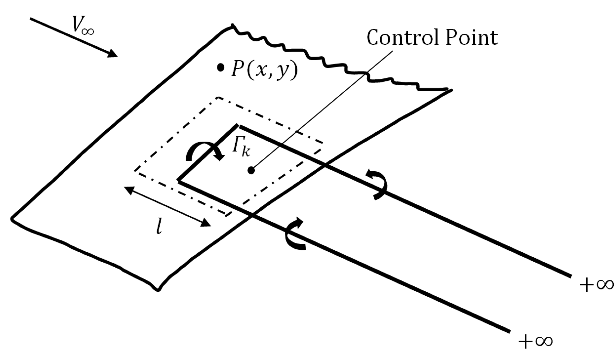
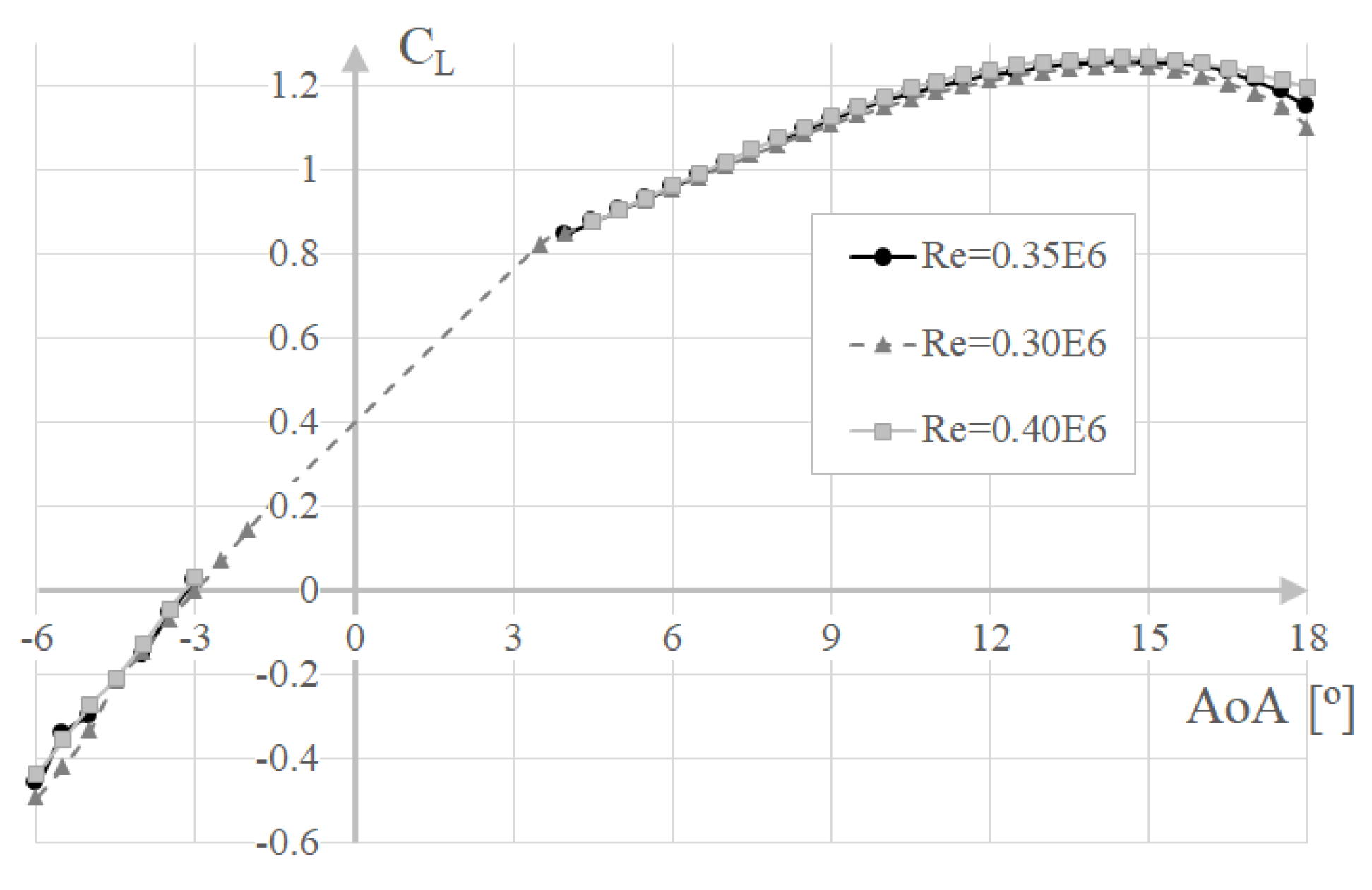
2.1.1. Aerodynamics
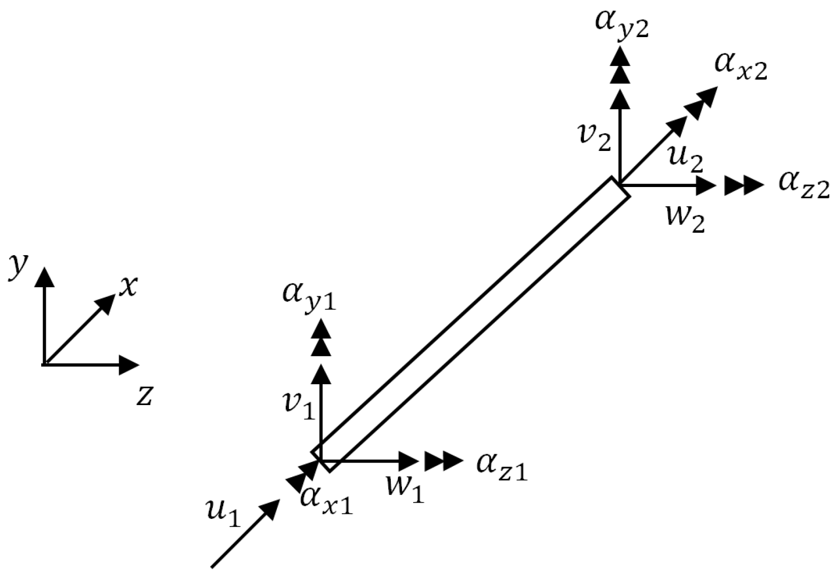
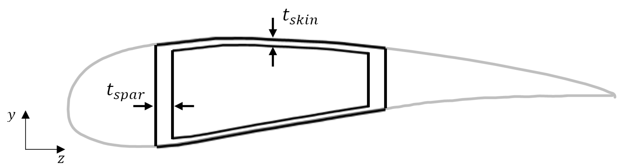
2.1.2. Structures
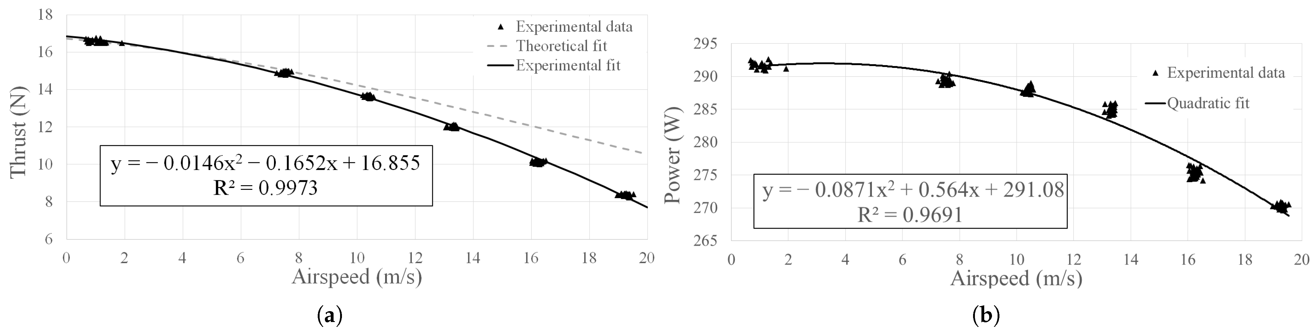
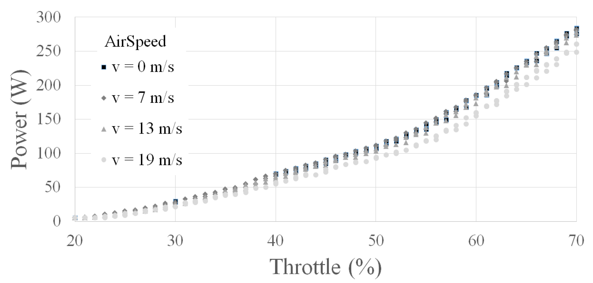
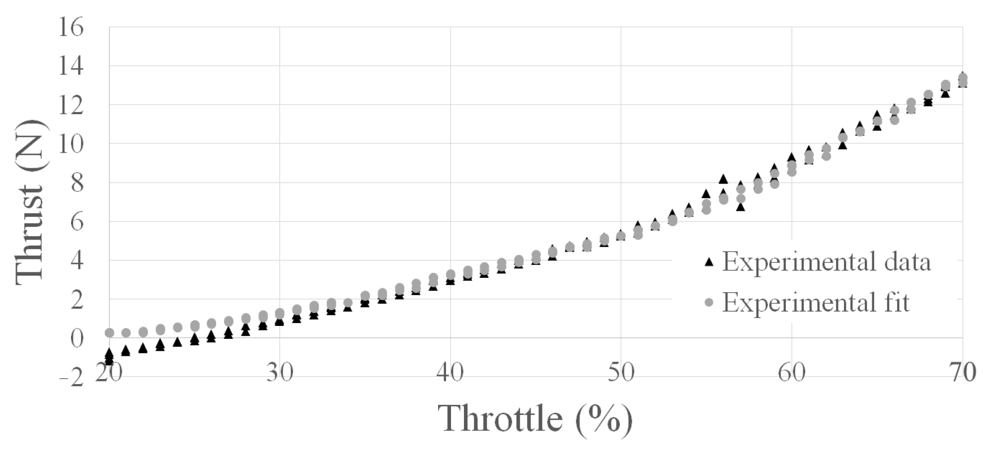
2.1.3. Propulsion
2.1.4. Trajectory Optimization Method
2.2. Competition Related Models
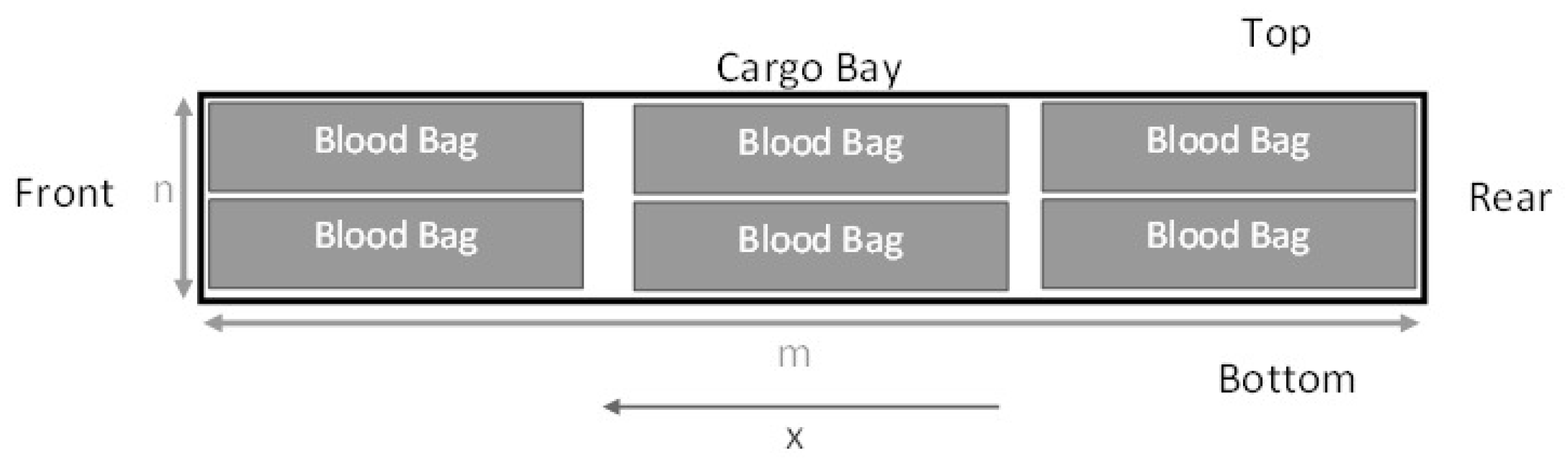
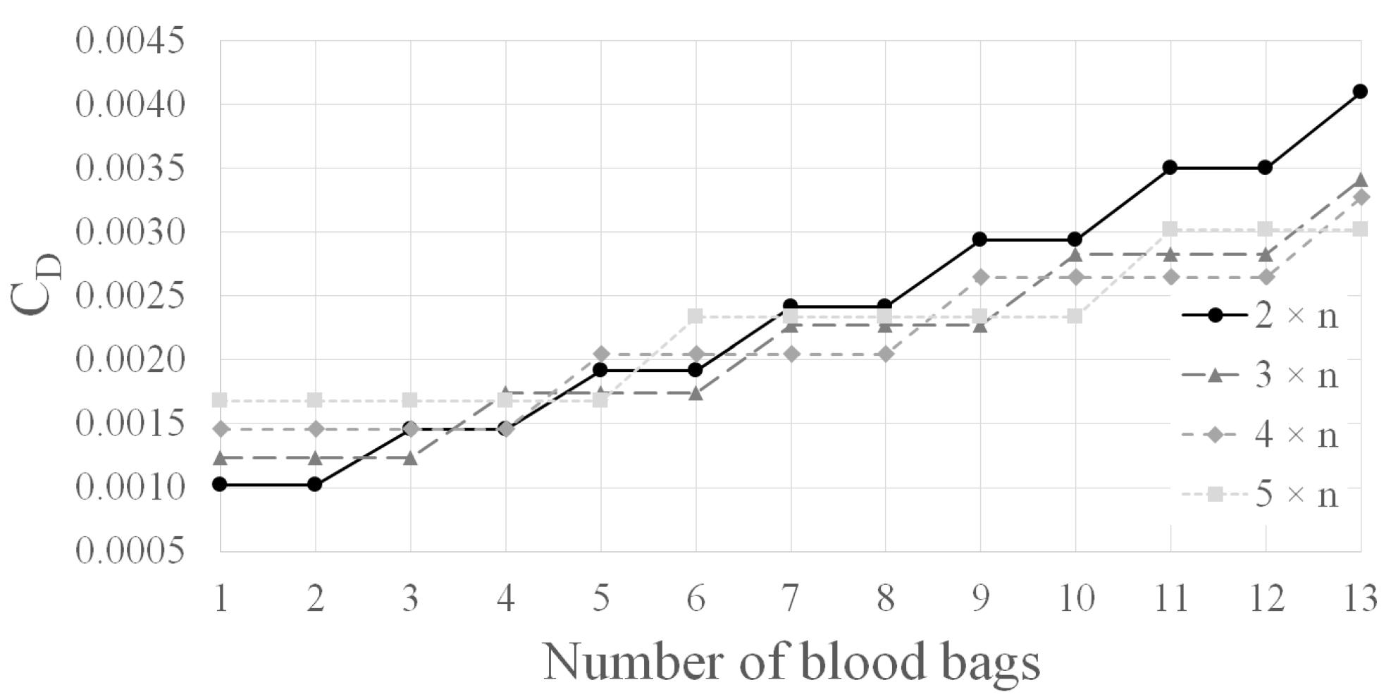
2.2.1. Cargo Bay Drag Model
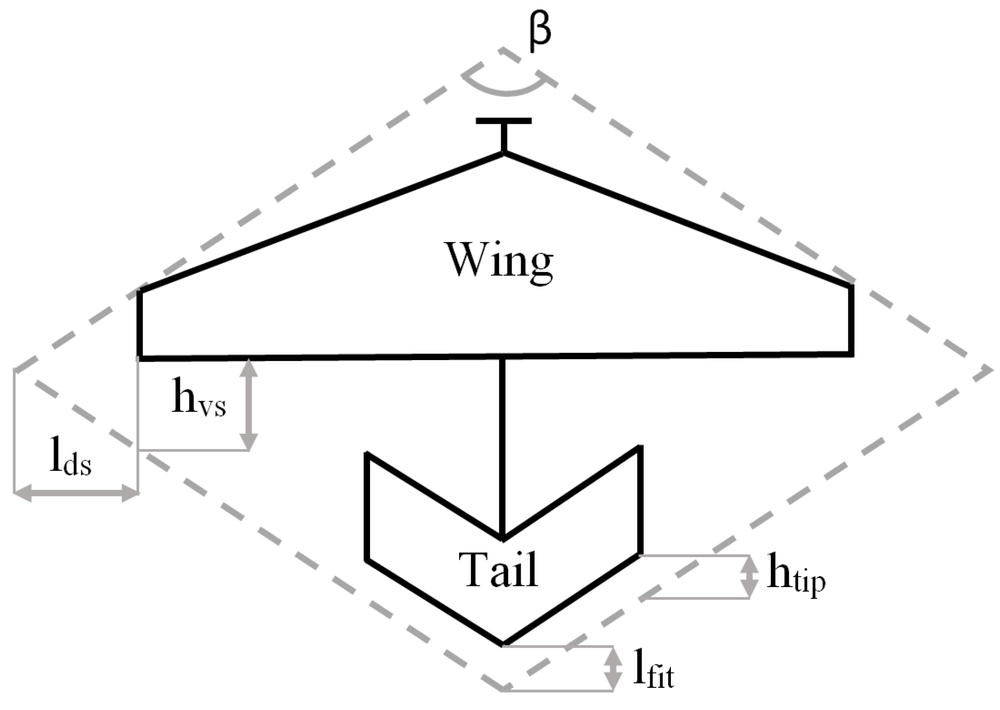
2.2.2. Rhombus Box Model
2.2.3. Trim and Stability Model
2.2.4. Take-Off Distance
2.3. Concurrent Design Framework
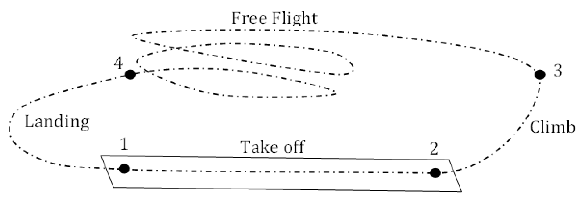
2.3.1. Flight Segments Integration and Competition Scoring
Take-Off Segment
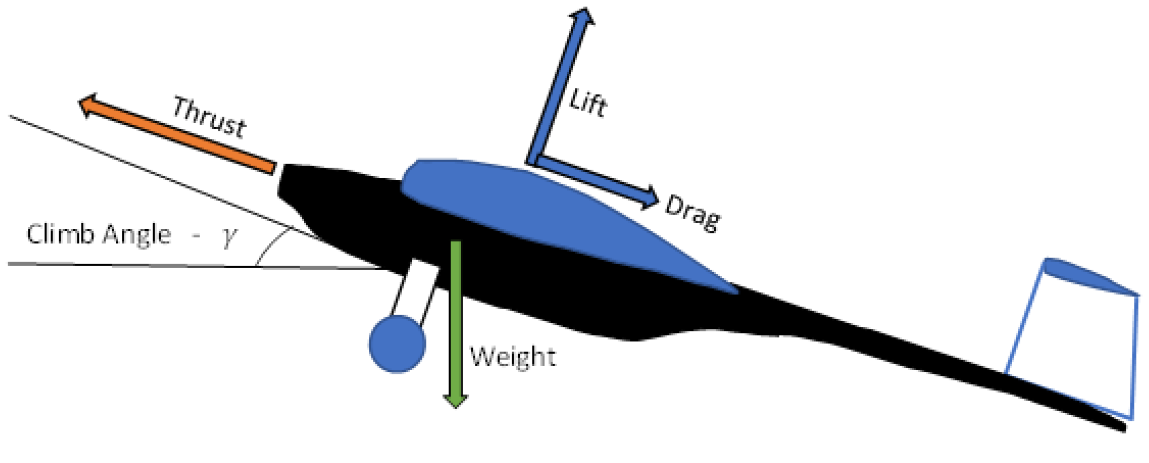
Climb Segment
Cruise Segment
Final Score
2.3.2. Problem Constraints
Box Size Constraints
Aerodynamic Constraints
Structural Constraints
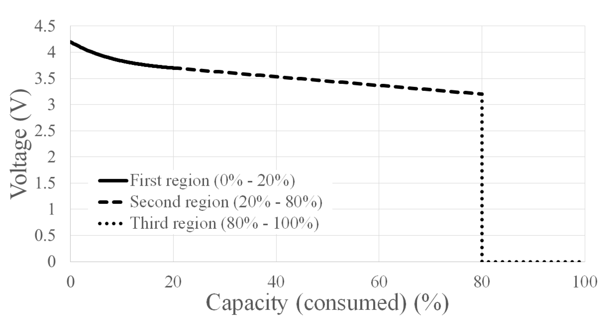
Energy Constraints
Payload Constraints
Trim and Stability Constraints
Trajectory Constraints
2.3.3. Aircraft and Trajectory Parameters
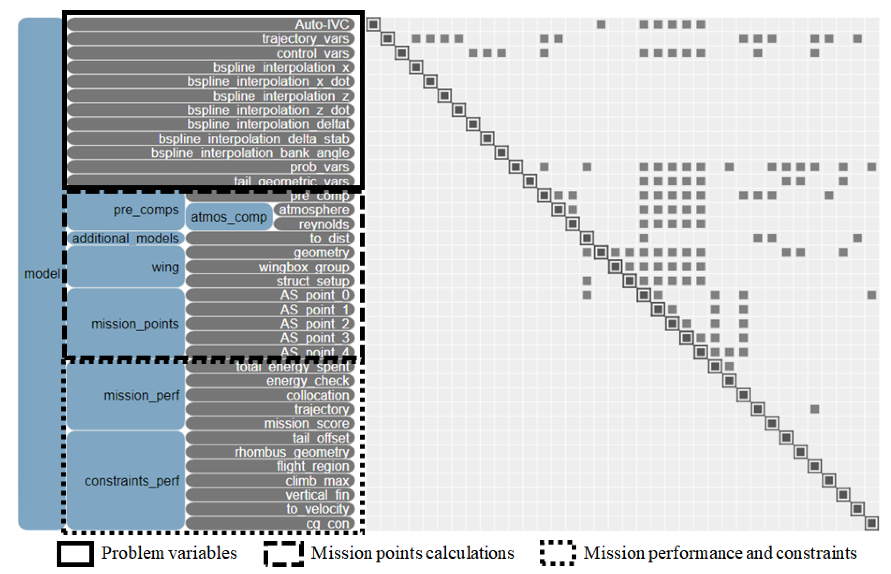
2.3.4. MDO Framework Architecture
Problem Variables
Mission Points
Mission Performance and Constraints
3. Results
3.1. Framework Parameters
3.2. Specialized Design Solutions
3.2.1. Payload Score Maximization
3.2.2. Climb Score Maximization
3.2.3. Distance Score Maximization
3.3. Optimal Design and Trajectory for Maximum Total Score
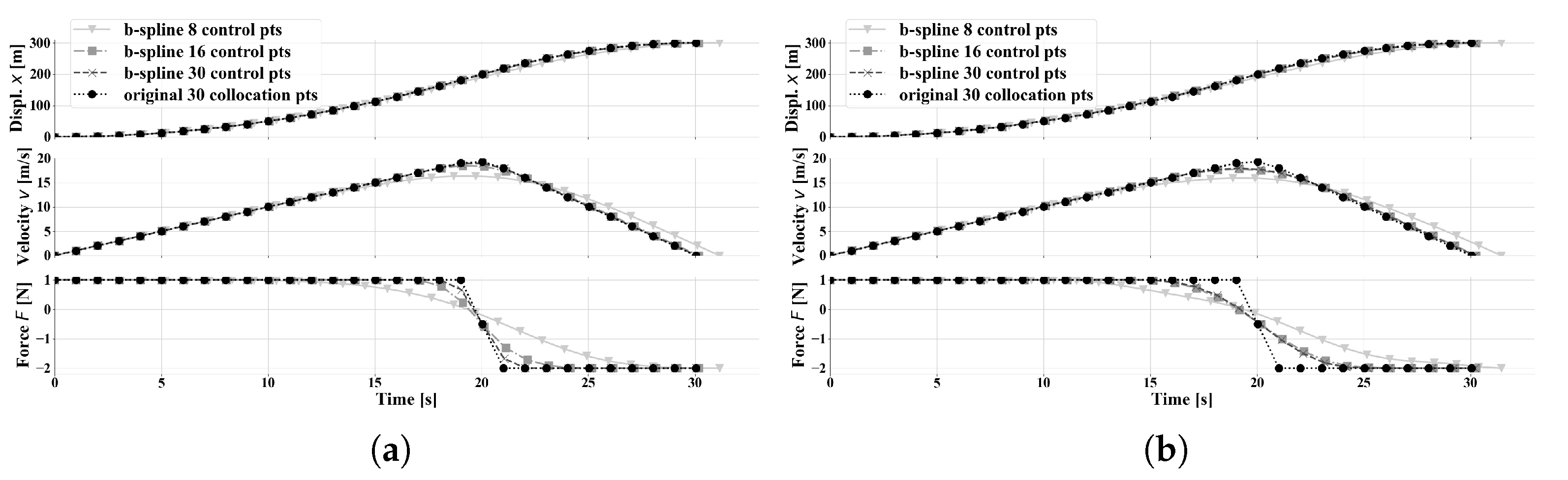
3.4. B-Spline Control Functions
4. Discussion
5. Conclusions
Author Contributions
Funding
Institutional Review Board Statement
Informed Consent Statement
Data Availability Statement
Conflicts of Interest
Abbreviations
| ACC | Air Cargo Challenge |
| CG | Center of Gravity |
| DOF | Degrees-of-Freedom |
| ESC | Electronic Speed Controller |
| FEM | Finite Element Model |
| KS | Kreisselmeier–Steinhauser |
| LiPo | Lithium-Polymer |
| MDA | Multidisciplinary Analysis |
| MDAO | Multidisciplinary Analysis and Design Optimization |
| MDF | Multidisciplinary Feasible |
| MDO | Multidisciplinary Design Optimization |
| NLBGS | Nonlinear Block Gauss-Seidel |
| VLM | Vortex Latice Method |
| XDSM | eXtended Design Structure Matrix |
References
- AkaModell München. Air Cargo Challenge 2022 Participation Handbook. Version 01.11. Available online: https://akamodell-muenchen.de/air-cargo-challenge-2022/regulations/ (accessed on 20 May 2022).
- Kontogiannis, S.G.; Mazarakos, D.; Kostopoulos, V. ATLAS IV wing aerodynamic design: From conceptual approach to detailed optimization. Aerosp. Sci. Technol. 2016, 56, 135–147. [Google Scholar] [CrossRef]
- Kovanis, A.P.; Skaperdas, V.; Ekaterinaris, J.A. Design and Analysis of a Light Cargo UAV Prototype. J. Aerosp. Eng. 2012, 25, 228–237. [Google Scholar] [CrossRef] [Green Version]
- Garcia, G.L.; Gamboa, P.V. Mass prediction models for air cargo challenge aircraft. Aeronaut. J. 2022, 126, 249–296. [Google Scholar] [CrossRef]
- Czyba, R.; Hecel, M.; Jabłoński, K.; Lemanowicz, M.; Płatek, K. Application of computer aided tools and methods for unmanned cargo aircraft design. In Proceedings of the IEEE 20th International Conference on Methods and Models in Automation and Robotics (MMAR), Miedzyzdroje, Poland, 24–27 August 2015. [Google Scholar] [CrossRef]
- Vrdoljak, M.; Prebeg, P.; Barać, M.I.; Andrić, M. Design and Human-in-the-loop Simulation of Radio Controlled Fixed Wing Aircraft. In Proceedings of the IEEE 5th International Conference on Smart and Sustainable Technologies (SpliTech), Split, Croatia, 23–26 September 2020. [Google Scholar] [CrossRef]
- Jameson, A.; Leoviriyakit, K.; Shankaran, S. Multi-Point Aero-Structural Optimization of Wings Including Planform Variations. In Proceedings of the 45th AIAA Aerospace Sciences Meeting, Reno, NV, USA, 8–11 January 2007. [Google Scholar] [CrossRef] [Green Version]
- Keidel, D.; Molinari, G.; Ermanni, P. Aero-structural optimization and analysis of a camber-morphing flying wing: Structural and wind tunnel testing. J. Intell. Mater. Syst. Struct. 2019, 30, 908–923. [Google Scholar] [CrossRef]
- Bons, N.P.; Martins, J.R.R.A. Aerostructural Design Exploration of a Wing in Transonic Flow. Aerospace 2020, 7, 118. [Google Scholar] [CrossRef]
- Salem, K.A.; Cipolla, V.; Palaia, G.; Binante, V.; Zanetti, D. A Physics-Based Multidisciplinary Approach for the Preliminary Design and Performance Analysis of a Medium Range Aircraft with Box-Wing Architecture. Aerospace 2021, 8, 292. [Google Scholar] [CrossRef]
- Raymer, D.P. Aicraft Design: A Conceptual Approach, 2nd ed.; American Institute of Aeronautics and Astronautics: Reston, VA, USA, 1992; ISBN 0-930403-51-7. [Google Scholar]
- You, C.; Zhang, R. 3D Trajectory Optimization in Rician Fading for UAV-Enabled Data Harvesting. IEEE Trans. Wirel. Commun. 2019, 18, 3192–3207. [Google Scholar] [CrossRef] [Green Version]
- Carabaza, S.; Scherer, J.; Rinner, B.; Lopez-Orozco, J.; Besada, E. UAV Trajectory Optimization for Minimum Time Search with Communication Constraints and Collision Avoidance. Eng. Appl. Artif. Intell. 2019, 85, 357–371. [Google Scholar] [CrossRef]
- Dobrokhodov, V.; Jones, K.; Walton, C.; Kaminer, I. Energy-Optimal Trajectory Planning of Hybrid Ultra-Long Endurance UAV in Time-Varying Energy Fields. In Proceedings of the AIAA Scitech 2020 Forum, Orlando, FL, USA, 6–10 January 2020. [Google Scholar] [CrossRef]
- Murrieta-Mendoza, A.; Romain, C.; Botez, R.M. 3D Cruise Trajectory Optimization Inspired by a Shortest Path Algorithm. Aerospace 2020, 7, 99. [Google Scholar] [CrossRef]
- Vitali, A.; Battipede, M.; Lerro, A. Multi-Objective and Multi-Phase 4D Trajectory Optimization for Climate Mitigation-Oriented Flight Planning. Aerospace 2021, 8, 395. [Google Scholar] [CrossRef]
- Martins, J.R.R.A.; Lambe, A. Multidisciplinary Design Optimization: A Survey of Architectures. AIAA J. 2013, 51, 2049–2075. [Google Scholar] [CrossRef] [Green Version]
- Burdette, D.; Martins, J.R.R.A. Design of a transonic wing with an adaptive morphing trailing edge via aerostructural optimization. Aerosp. Sci. Technol. 2018, 81, 192–203. [Google Scholar] [CrossRef]
- Brooks, T.R.; Martins, J.R.R.A.; Kennedy, G.J. High-fidelity Aerostructural Optimization of Tow-steered Composite Wings. J. Fluids Struct. 2019, 88, 122–147. [Google Scholar] [CrossRef]
- Chauhan, S.S.; Martins, J.R.R.A. Tilt-wing eVTOL takeoff trajectory optimization. J. Aircr. 2020, 57, 93–112. [Google Scholar] [CrossRef]
- Jasa, J.P.; Brelje, B.J.; Gray, J.S.; Mader, C.A.; Martins, J.R.R.A. Large-Scale Path-Dependent Optimization of Supersonic Aircraft. Aerospace 2020, 7, 152. [Google Scholar] [CrossRef]
- Jasa, J.P.; Hwang, J.T.; Martins, J.R.R.A. Open-source coupled aerostructural optimization using Python. Struct. Multidiscip. Optim. 2018, 57, 1815–1827. [Google Scholar] [CrossRef]
- Anderson, J. Fundamentals of Aerodynamics, 6th ed.; McGraw-Hill: New York, NY, USA, 2016; ISBN 978-1259129919. [Google Scholar]
- Zucco, G.; Oliveri, V.; Rouhi, M.; Telford, R.; Peeters, D.; Clancy, G.; McHale, C.; O’Higgins, R.; Young, T.; Weaver, P. Static Test of a Variable Stiffness Thermoplastic Composite Wingbox under Shear, Bending and Torsion. Aeronaut. J. 2019, 124, 635–666. [Google Scholar] [CrossRef]
- Chauhan, S.S.; Martins, J.R.R.A. Low-Fidelity Aerostructural Optimization of Aircraft Wings with a Simplified Wingbox Model Using OpenAeroStruct. In Proceedings of the 6th International Conference on Engineering Optimization, EngOpt 2018, Lisboa, Portugal, 17–19 September 2018; pp. 418–431. [Google Scholar] [CrossRef]
- Traub, L. Calculation of Constant Power Lithium Battery Discharge Curves. Batteries 2016, 2, 17. [Google Scholar] [CrossRef] [Green Version]
- Kelly, M. An Introduction to Trajectory Optimization: How to Do Your Own Direct Collocation. SIAM Rev. 2017, 59, 849–904. [Google Scholar] [CrossRef]
- Betts, J.T. Survey of Numerical Methods for Trajectory Optimization. J. Guid. Control. Dyn. 1998, 21, 193–207. [Google Scholar] [CrossRef]
- Morgado, F.; Marta, A.C.; Gil, P. Multi-stage rocket preliminary design and trajectory optimization using a multidisciplinary approach. Struct. Multidiscip. Optim. 2022, 65, 192. [Google Scholar] [CrossRef]
- Becerra, V.M. Practical Direct Collocation Methods for Computational Optimal Control. In Modeling and Optimization in Space Engineering; Springer: New York, NY, USA, 2013; Volume 73, pp. 33–60. [Google Scholar] [CrossRef]
- Liem, R.; Kenway, G.; Martins, J.R.R.A. Multimission Aircraft Fuel-Burn Minimization via Multipoint Aerostructural Optimization. AIAA J. 2015, 53, 104–122. [Google Scholar] [CrossRef] [Green Version]
- Kamien, M.I.; Schwartz, N.L. Dynamic Optimization, 2nd ed.; Advanced Textbooks in Economics; Elsevier: Amsterdam, The Netherlands, 1991; ISBN 0-444-01609-0. [Google Scholar]
- Gudmundson, S. General Aviation Aircraft Design: Applied Methods and Procedures; Elsevier: Amsterdam, The Netherlands, 2014; Volume 1, ISBN 9780123973085. [Google Scholar]
- Götten, F.; Havermann, M.; Braun, C.; Marino, M.; Bil, C. Improved Form Factor for Drag Estimation of Fuselages with Various Cross Sections. J. Aircr. 2021, 58, 549–561. [Google Scholar] [CrossRef]
- Hoerner, S.F. Fluid-dynamic Drag: Practical Information on Aerodynamic Drag and Hydrodynamic Resistance; Hoerner Fluid Dynamics: Brick Town, NJ, USA, 1965. [Google Scholar]
- Schlichting, H.; Gersten, K. Boundary-Layer Theory, 8th ed.; Springer: Berlin/Heidelberg, Germany, 2000; ISBN 978-3-642-85829-1. [Google Scholar]
- Deperrois, A. XFLR5. Available online: http://www.xflr5.tech/xflr5.htm (accessed on 20 May 2022).
- Kreisselmeier, G.; Steinhauser, R. Systematic Control Design by Optimizing a Vector Performance Index. IFAC Proc. Vol. 1979, 12, 113–117. [Google Scholar] [CrossRef]
- GoodFellow. Carbon/Epoxy Composite—Material Information. Available online: http://www.goodfellow.com/A/Carbon-Epoxy-Composite.html (accessed on 20 May 2022).
- Benaouali, A.; Kachel, S. Multidisciplinary design optimization of aircraft wing using commercial software integration. Aerosp. Sci. Technol. 2019, 92, 766–776. [Google Scholar] [CrossRef]
- Molinari, G.; Arrieta, A.F.; Ermanni, P. Aero-Structural Optimization of Three Dimensional Adaptive Wings with Embedded Smart Actuators. AIAA J. 2014, 52, 1940–1950. [Google Scholar] [CrossRef]
- Martins, J.R.R.A.; Ning, A. Engineering Design Optimization; Cambridge University Press: Cambridge, UK, 2022; ISBN 978-1108833417. [Google Scholar]
- Lambe, A.; Martins, J.R.R.A. Extensions to the Design Structure Matrix for the Description of Multidisciplinary Design, Analysis, and Optimization Processes. Struct. Multidiscip. Optim. 2012, 49, 273–284. [Google Scholar] [CrossRef]
- Gray, J.; Hwang, J.; Martins, J.R.R.A.; Moore, K.; Naylor, B. OpenMDAO: An open-source framework for multidisciplinary design, analysis, and optimization. Struct. Multidiscip. Optim. 2019, 59, 1075–1104. [Google Scholar] [CrossRef]
- Lewis, R.; Shubin, G.; Cramer, E.; Dennis, J.; Frank, P.; Michael, R.; Gregory, L.; Shubin, R. Problem Formulation for Multidisciplinary Optimization. SIAM J. Optim. 1997, 4, 754–776. [Google Scholar] [CrossRef]


| Control Points | Control B-Spline | State B-Splines + Control 16 Cp Spline | ||
|---|---|---|---|---|
| Func Evals | Obj | Func Evals | Obj | |
| 8 | 21 (−83.3%) | 31.0 (+3.7%) | 182 (+44.4%) | 31.4 (+5.2%) |
| 16 | 20 (−84.1%) | 30.0 (+0.5%) | 98 (−22.2%) | 30.3 (+1.3%) |
| 30 | 21 (−83.3%) | 29.9 (+0.2%) | 66 (−47.6%) | 30.2 (1.1%) |
| Variable | Meaning | Type | Control Points | Value/Bounds | |
|---|---|---|---|---|---|
| Box size | tail-wing distance | design | - | [] m | |
| rhombus box angle | design | - | [70, 140] | ||
| lat. diag. avail. space | constraint | - | >0 | ||
| vert. space avail. at tip | constraint | - | >0 | ||
| tail diag. avail. space | constraint | - | >0 | ||
| tail avail. space at tip | constraint | - | >0 | ||
| Wing | span | design | - | [1, 3] m | |
| dihedral angle | fixed design | - | 0 | ||
| sweep angle | design | - | [−5, 30] | ||
| lift coeff. at 0° AoA | constant | - | 0.4 | ||
| parasite drag coeff. | constant | - | 0.008 | ||
| 2D lift coeff. | constraint | - | <1.3 | ||
| max. thick.-to-chord | constant | - | 0.2533 | ||
| spar thickness | design | 2 | [0.15, 1] mm | ||
| skin thickness | design | 2 | [0.15, 1] mm | ||
| thickness-to-chord | design | 2 | [0.08, 0.12] | ||
| chord | design | 3 | [0.05, 0.4] m | ||
| twist | design | 3 | [−5, 5] | ||
| KS failure function | constraint | - | <0 | ||
| Tail | span | design | - | [0.1, 0.6] m | |
| dihedral angle | design | 1 | [20, 80] | ||
| sweep angle | design | - | [−3, 10] | ||
| lift coeff. at 0° AoA | constant | - | 0 | ||
| parasite drag coeff. | constant | - | 0.006 | ||
| 2D lift coeff. | constraint | - | 0.95 | ||
| max. thick.-to-chord | constant | - | 0.2953 | ||
| thickness | constant | 1 | 0.09 | ||
| tube thickness | design | 1 | [0.15, 0.5] mm | ||
| chord | design | 2 | [0.05, 0.25] m | ||
| twist | constant | 1 | 0 | ||
| KS failure function | constraint | - | <0 | ||
| tube intersection | constraint | - | <0 | ||
| Energy | battery capacity | design | - | [2, 10] A h | |
| specific energy | constant | - | 600,000 J kg | ||
| usable energy factor | constant | - | 60% | ||
| max. capacity | constraint | - | - | ||
| max. energy | constraint | - | - | ||
| Mass | wing/tailless struct. weight | constant | - | 1.0 kg | |
| empty CG | fixed design | - | [0, 0, 0] | ||
| battery weight | design | - | [0.2, 2] kg | ||
| payload weight | design | - | [0, 4] kg | ||
| payload CG | constraint | - | [−1 to 1, 0, 0] mm | ||
| Take-off | take-off lift coeff. | constant | - | 0.3 | |
| take-off drag coeff. | constant | - | 0.02 | ||
| max. lift coeff. | constant | - | 1.5 (with flaps) | ||
| track friction coeff. | constant | - | 0.07 | ||
| Stab. | pitching moment coeff. | constraint | - | [] | |
| tail volume coeff. | constraint | - | [0.04, 0.09] |
| Variable | Meaning | Type | Control Points | Value/Bounds | |
|---|---|---|---|---|---|
| Trajectory | x | horizontal displacement | design | n | [0, 10,000] m |
| z | vertical displacement | design | n | [0, 120] m | |
| horizontal velocity | design | n | [0, 25] m s | ||
| vertical velocity | design | n | [0, 18] m s | ||
| elapsed time | constant | - | 180 s | ||
| throttle | design | n | [0, 1] | ||
| stabilator angle | design | n | [−25, 25] | ||
| angle of attack | design | n | [−15, 15] | ||
| horiz. displacement defect | constraint | - | [] | ||
| vert. displacement defect | constraint | - | [] | ||
| horizontal force defect | constraint | - | [] | ||
| vertical force defect | constraint | - | [] |
| Objective | Payload | Climb | Distance | Total | Total Bspline | |
|---|---|---|---|---|---|---|
| Payload score | 692.3 | 76.9 | 0.0 | 846.2 | 1000.0 | |
| Climb score | 615.5 | 943.6 | 638.8 | 920.8 | 922.3 | |
| Distance score | 656.3 | 929.4 | 930.1 | 700.7 | 721.2 | |
| Total score | 2160.5 | 2144.9 | 1725.8 | 2714.4 | 2907.8 | |
| Payload bags | 9 () | 1 () | 0 () | 11 () | 13 () | |
| Height | [m] | 37.74 | 114.30 | 39.72 | 116.56 | 77.67 |
| Distance | [m] | 2829.4 | 4006.5 | 4019.4 | 3001.6 | 3097.4 |
| Wing area | [m] | 0.720 | 0.141 | 0.137 | 0.721 | 0.732 |
| Wing aspect ratio | 4.50 | 13.47 | 17.26 | 4.51 | 4.58 | |
| Wing taper ratio | 1.00 | 0.25 | 0.31 | 1.00 | 1.00 | |
| Tail area | [m] | 0.150 | 0.030 | 0.025 | 0.150 | 0.150 |
| Total weight | [kg] | 4.468 | 1.926 | 1.877 | 5.227 | 5.653 |
| Tail-wing distance | [m] | 0.601 | 0.600 | 0.601 | 0.601 | 0.601 |
| Rhombus box | [] | 103.7 | 112.4 | 122.9 | 105.8 | 111.8 |
| Wing span | [m] | 1.800 | 1.380 | 1.535 | 1.803 | 1.831 |
| Wing sweep | [] | 0.04 | 0.00 | 0.00 | 1.01 | 0.22 |
| Wing spar thickness | [mm] | (0.15,0.16) | (0.17,0.44) | (1.0,1.0) | (0.15,0.15) | (0.15,0.15) |
| Wing skin thickness | [mm] | (0.15,0.18) | (0.21,0.72) | (1.0,1.0) | (0.15,0.15) | (0.15,0.15) |
| Wing thick.-to-chord | [%] | (8.0,8.0) | (11.2,8.5) | (11.2,11.9) | (8.0,8.0) | (8.2,8.0) |
| Wing chord | [m] | 0.400 | 0.102 | 0.089 | 0.400 | 0.400 |
| Tail span | [m] | 0.600 | 0.393 | 0.419 | 0.600 | 0.600 |
| Tail dihedral | [] | 35.1 | 35.0 | 35.0 | 35.2 | 36.5 |
| Tail sweep | [] | −0.1 | 0.0 | 0.0 | −0.1 | −0.9 |
| Tail tube thickness | [mm] | 0.15 | 0.31 | 0.43 | 0.36 | 0.15 |
| Tail chord | [m] | 0.250 | 0.077 | 0.060 | 0.250 | 0.250 |
| Empty | [kg] | 1.472 | 1.362 | 1.497 | 1.466 | 1.453 |
| Battery capacity | [mA h] | 2779 | 2778 | 2778 | 2778 | 2778 |
| Battery mass | [kg] | 0.200 | 0.200 | 0.200 | 0.200 | 0.200 |
| Payload | [kg] | 2.996 | 0.364 | 0.180 | 3.561 | 4.000 |
| Iterations | 30 | 98 | 33 | 179 | 186 | |
| CPU time | [h] | 1.21 | 3.92 | 1.33 | 7.08 | 6.22 |
Publisher’s Note: MDPI stays neutral with regard to jurisdictional claims in published maps and institutional affiliations. |
© 2022 by the authors. Licensee MDPI, Basel, Switzerland. This article is an open access article distributed under the terms and conditions of the Creative Commons Attribution (CC BY) license (https://creativecommons.org/licenses/by/4.0/).
Share and Cite
Matos, N.M.B.; Marta, A.C. Concurrent Trajectory Optimization and Aircraft Design for the Air Cargo Challenge Competition. Aerospace 2022, 9, 378. https://doi.org/10.3390/aerospace9070378
Matos NMB, Marta AC. Concurrent Trajectory Optimization and Aircraft Design for the Air Cargo Challenge Competition. Aerospace. 2022; 9(7):378. https://doi.org/10.3390/aerospace9070378
Chicago/Turabian StyleMatos, Nuno M. B., and Andre C. Marta. 2022. "Concurrent Trajectory Optimization and Aircraft Design for the Air Cargo Challenge Competition" Aerospace 9, no. 7: 378. https://doi.org/10.3390/aerospace9070378