1. Introduction
The interest in developing Prognostics and Health Maintenance (PHM) applications is growing in some industries aiming to reduce maintenance costs and down time [
1]. In the aviation industry, the interest has also emerged due to the need for accomplishing strict safety and operational reliability policies [
2].
Taking advantage of the profusion of sensors present on modern aircraft, the collection and the analysis of Condition Monitoring (CM) data has been useful to develop data-driven models [
1,
3]. In consequence, maintenance processes are assisted by such models, which usually leverage the advantages of Artificial Intelligence (AI) and Machine Learning (ML). Particularly, Predictive Maintenance (PM) strategies have been used to determine the advent of a failure by applying Remaining Useful Life (RUL) concepts [
4,
5,
6,
7], i.e., methods that predict of the remaining time an equipment is estimated to be able to function without failing [
8].
In the development of data-driven RUL estimation models, data gathering is mainly focused on (1) getting run-to-failure data [
9], and (2) collecting many failure instances [
3]. While the first aims to collect data related to the transition from healthy to faulty states, the second aims to identify health degradation patterns.
Data transformations from time or frequency domains have often been used to discover trends that sensor signals usually conceal [
6,
10]. Such aircraft sensor signals are frequently non-stationary [
8,
11], i.e., time period and frequency are not constant [
12]. Hence, data transformation on both domains has been proposed [
7,
13,
14]. Unfortunately, there are cases in which the failure advent is generally unable to be observed directly from data. In such cases, the construction of physics-based Health Indicators (HIs) can play a significant role [
15,
16].
The construction of HIs has been considered an essential stage in PHM, mainly when outputs of a physics-based model are used as inputs for data-driven models. In literature, the integration of two different model types is referred to as the construction of hybrid approaches [
15]. When data-driven approaches use ML under a supervised learning approach, data labeling has been challenging because a degradation curve has to be proposed [
15,
17]. This process is usually known as the health stage division process and its main goal is to identify multiple health stages that could be identified along the equipment lifetime.
Among the main contributions of this work are: (1) the inclusion of physics-based models with data-driven models within a PHM program; (2) a Health Indicator construction approach based on time and frequency domains; (3) the identification of two degradation stages experienced by aircraft cooling units; and (4) the RUL estimation for those units.
This work mainly draws attention to the second contribution because it presents a time-frequency data transformation oriented for non-stationary signals. Concretely, our time-frequency HI construction approach based on the Hilbert spectrum [
18,
19] is used to accumulate the lowest frequency instances. Our experiments, conducted using data from the Cooling System (CS) of a wide body aircraft fleet [
1], suggest that the degradation of Cooling Units (CUs) may be related to the presence of periods with the lowest frequency instances. Our RUL estimations, inferred from a Neural Network (NN) based model have been more precise after prioritizing the health prognostics of the last flight hours.
This article is organized as follows.
Section 2 presents the literature review regarding RUL estimation approaches and time-frequency data transformation.
Section 3 describes the developing phases and the modules of the proposed PHM program that integrates physics-based and data-driven models.
Section 4 details the data gathered from a wide body aircraft fleet and the failure instances associated with the Cooling System. The development of the RUL predictor model is described into three sections: Health Indicator (HI) construction (
Section 5), Health Stage division (
Section 6) and RUL estimation (
Section 7). The RUL estimations obtained by using the proposed HI construction versus using raw data are compared in
Section 8. Finally, the conclusions and future lines of research are presented in
Section 9.
2. Literature Review and Background
2.1. RUL Prediction Approaches
Several studies have reviewed common RUL prediction approaches and classified them into various categories taking different emphases [
12,
20,
21,
22,
23,
24]. Considering the basic techniques and methodologies, the following four categories have been proposed in [
15]: physics-based, statistical-based, data-driven, and hybrid approaches.
Physics-based approaches describe the advent of a failure through mathematical models [
24]. Statistical-based estimate the RUL by establishing models based on empirical knowledge and present the RUL prediction as a conditional Probabilistic Density Function (PDF) [
22]. Data-driven approaches typically attempt to learn degradation patterns using Artificial Intelligence (AI)/Machine Learning (ML) techniques from run-to-failure data [
12,
21,
22,
25]. Finally, hybrid approaches aim to integrate the capabilities of two or more previous approaches [
15].
Given the availability of Condition Monitoring (CM) data, usually gathered from digital twin systems (e.g., data from the Commercial Modular Aero-Propulsion System Simulation (CMAPSS) [
8,
11]), industrial and academic researchers have extended the literature related to developing data-driven models.
Among the main reasons for adopting data-driven approaches is the fact that health degradation can be revealed from data, avoiding PHM practitioners the necessity to delve into the physics of the signals analyzed [
10], which is usually complex. That advantage has allowed researchers to be focused into performing adequate data transformations to learn the health degradation path through AI/ML techniques [
6]. Unfortunately, there are cases in which data transformations from time or frequency domains are not sufficient to develop data-driven models.
2.2. Time-Frequency Data Transformations
Data transformations from time or frequency domains, such are kurtosis, mean, peaks, and Fourier transform, among others, have been widely used in the presence of stationary signals [
6,
7]. Nevertheless, data transformations on a single domain have demonstrated limitations in the analysis of non-stationary signals and non-linear systems [
24].
When the degree of a time-frequency moment can be interpreted and moments can be useful to predict health states, obtaining the following moments is suggested: conditional spectral moment, conditional temporal moment and joint time-frequency moment [
3,
26]. Otherwise, time-frequency data transformations, such as, Short-time Fourier Transform (STFT) [
27], Wigner-Ville Distribution (WVD) [
14], Empirical Mode Decomposition (EMD) [
13] and Hilbert spectrum [
18] can be promising alternatives.
In time-frequency analysis, Fast Fourier (FF) transform has been widely used [
28]. In prognostics, STFT has been used to identify the advent of failures from the power spectrum. However, FF has physical meaning for linear systems, i.e., systems in which the change of the outputs is somehow proportional to the change of the inputs [
10,
13,
29].
As an alternative, WVD has been considered as the most prominent time-frequency representation since it satisfies an exceptionally large number of mathematical properties [
14]. Moreover, its applicability can be extended to multidimensional vectors. However, in the presence of large amounts of data, WVD is less powerful given that the computational cost can be high due to redundancies in the Fourier Transform (FT) computation [
30]. As an alternative, the time-frequency distribution, Hilbert spectrum, can be promising, since it is a distribution of signal amplitude that helps in distinguishing a mixture of moving signals [
18]. However, when the advent of a failure cannot be directly observed from time-frequency data transformation, even using AI/ML techniques, the need for developing hybrid approaches gains importance [
12,
15,
20].
3. Approach
The hybrid PHM program, proposed and implemented in this work, constructs HIs from a physics-based model and uses them as input signals of a data-driven model. Since the implementation of hybrid approaches is recommended when a single approach is not able to satisfactorily predict the RUL, the need of describing a general prognostics program gains interest. In
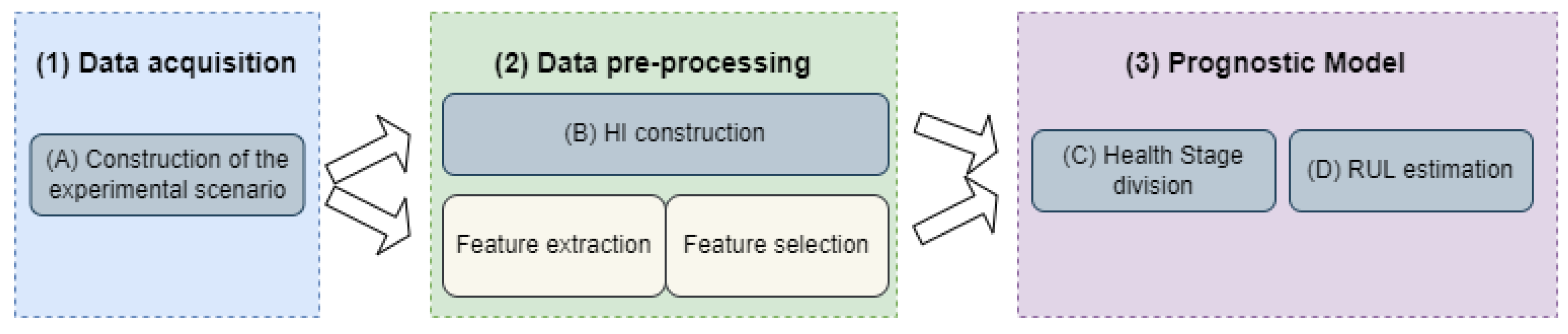
Figure 1, we illustrate the development stages and the modules for constructing physic-based and/or data-driven RUL predictors.
The backbone of our PHM program is composed of three prognostics stages presented in [
4]. Those main stages (dotted line boxes) are: (1) Data acquisition; (2) Data pre-processing; and, (3) Prognostic model phase. This prognostics process flow has been conceived to estimate the RUL by applying only data-driven approaches. For that reason, we adopted the PHM modules processes (gray boxes) presented in [
15] to construct hybrid approaches, namely:
data acquisition;
HI construction;
Health Stage division; and,
RUL estimation.
Our PHM program suggests adopting the data pre-processing modules (yellow boxes) when possible. In case the data-driven models do not achieve prognostics expectations, such is the case of the present work, the HI construction module can be adopted when health degradation is unable to be illustrated from data. In the listed modules, presented in the next sections, we performed the following technical processes, A to D, detailed in the following sections:
- A.
Data acquisition: refers mainly to constructing the experimental scenario. The main goal of this stage is to acquire run-to-failure data (
Section 4.1). This stage integrates data transformations (
Section 4.2), such as, data noise reduction, and data cleaning, before applying feature engineering techniques [
6]. In this technical process, handling imbalanced data (
Section 4.3) and defining training and testing samples (
Section 4.4) supports the prognostics model stage.
- B.
HI construction: refers to data transformations conducted by signal processing (
Section 5.1,
Section 5.2 and
Section 5.3) or AI/ML techniques [
15]. Feature engineering modules, such as, feature extraction, and feature selection, aim to extract and select the indicators that better describe the machinery degradation [
31,
32].
- C.
Health Stage division: considers different health stages, according to the varying degradation trends of HIs [
15]. Considering two health stages, the problem of finding the point that separates them is well known as
elbow point detection [
17].
- D.
RUL estimation: refers to the development of an AI/ML technique capable of predicting the RUL within health stages that present obvious degradation trends.
4. Experimental Scenario
This section refers to the tasks performed on the
Data acquisition stage. In this case, run-to-failure data was acquired from the Cooling System (CS) of a wide body aircraft fleet. The data was obtained from the project Real-Time Condition-based Maintenance for Adaptative Maintenance Planning-ReMAP of the European Union’s Horizon 2020 [
33].
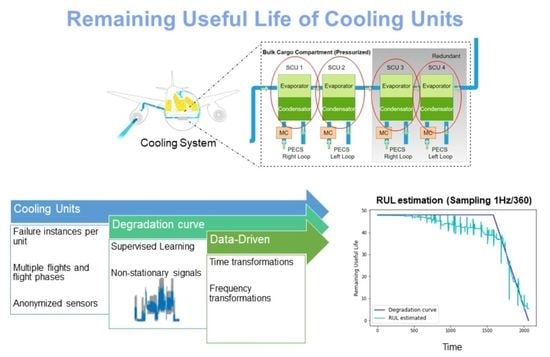
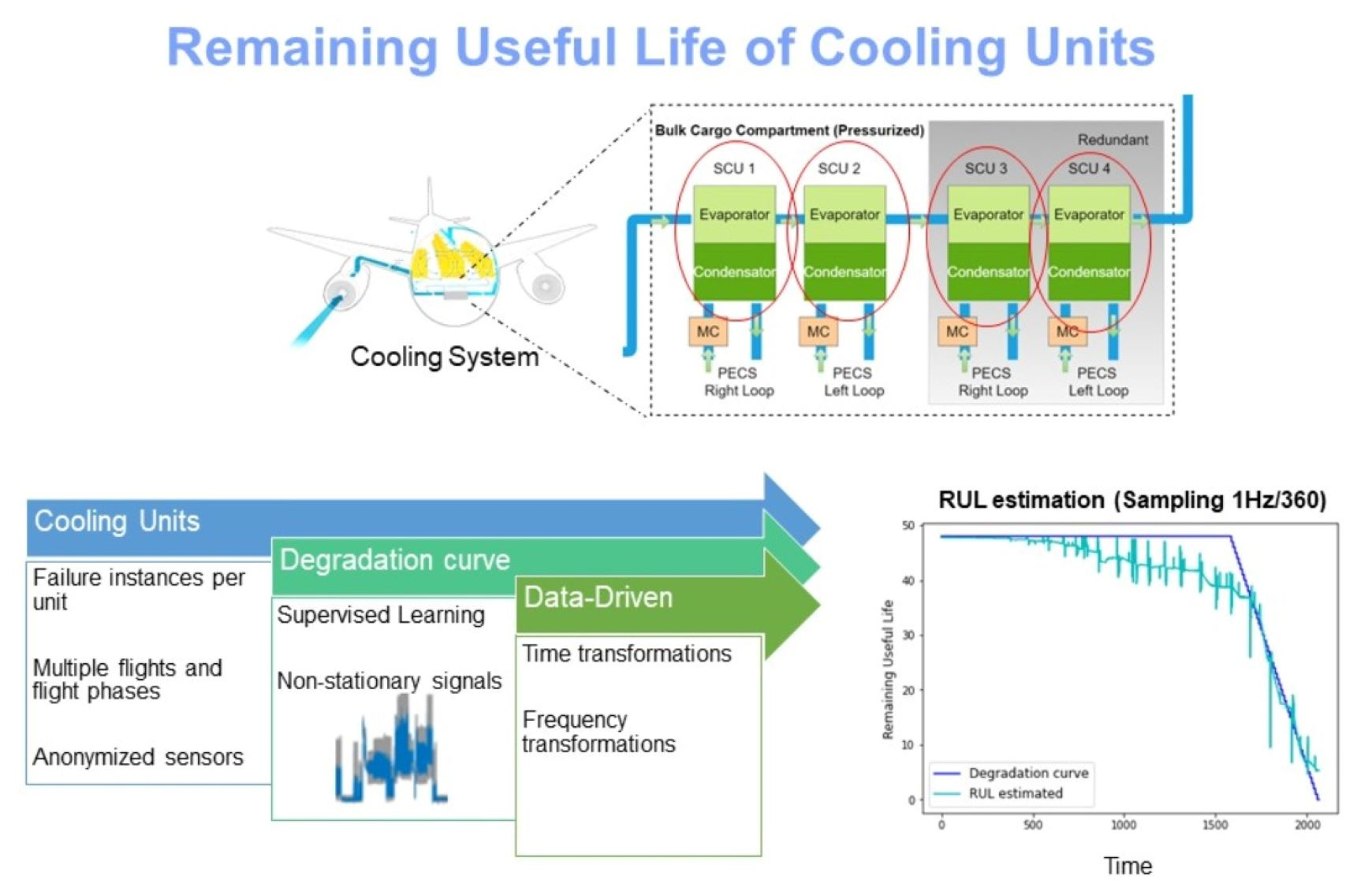
We consider using ReMAPs data to develop health prognostics of real aircraft systems and assist technicians in maintenance decision-making related to the CS. This cooling system senses the temperature of the wide body aircraft to maintain its operability. Specifically, the temperature is regulated by transporting liquid cooling through pumps, cooling units (CUs) and motor controllers.
As the Remaining Useful Life (RUL) concept was adopted to predict the amount of time left before an aircraft system fails [
8], we considered measuring the time in terms of remaining flight hours. Flight hours as an unit of time has been used in aerospace studies [
2,
34,
35]. Particularly, we are interested in predicting the RUL of CUs because the personal staff have documented the failure instances of these units.
For the ReMAP project, CSs of 17 different aircraft were monitored along 14 different flight phases using a sample rate of 1 Hz. During 29 months, data from 18,295 flights were collected, gathering 26.4 GB of data. Among sensor data, the personal staff has also documented maintenance interventions of three types of failures, namely: Flight Deck Events (FDE), Aircraft Technical Log (ATL) and Predictive Maintenance (PM) provided by technicians.
Only PM failures were used to monitor the health status because FDE and ATL failures were not confirmed by maintenance technicians. Despite 40 PM failures on CUs having occurred, only the analysis of 21 failures was considered because 2 failures were labeled as “dubious”, 10 were labeled as “likely”, while the remaining 7 did not present sensor data or presented constant measurements on sensors.
The CS of a single aircraft is monitored through 36 sensors located at four equivalent CUs. Therefore, each CU is monitored by analyzing 9 sensor signals. Among these signals, informative fields such as flight ID, departure data time, flight phase, row number, altitude and airspeed were also considered to monitor the CU health status along the different flights phases.
4.1. Construction of Run-to-Failure Data
The retrieved data does not provide run-to-failure data by default; CS data has to be ordered first. The flight ID, departure data time, flight phase and row number fields are used to order the data. To get run-to-failure data, we assume that technicians intervened CUs just when their useful life ended. That is, the failure threshold was defined as the last operating measurement before a maintenance intervention.
Under this assumption, we can get a run-to failure trajectory per aircraft CU. To get the different trajectories, we get the flights (flight ID), a previous maintenance intervention of each aircraft tail, and then sort the sensor measurements by row number. For easy understanding, each run-to-failure trajectory has been linked to the associated failure (failure ID). In
Table 1, the aircraft tail, the number of measurements and the number of flight hours for each trajectory are detailed. Note that the 21 trajectories presented are sorted by flight hours.
4.2. Noise Reduction and Data Cleaning
Cooling Units are monitored by 9 equivalent sensors. However, 3 of them presented a lot of infinite and NaN measurements, hampering their analysis. The fields, which where discarded from the first CU, correspond to xtooix*, wqybtv* and ytauwt*. Equivalent sensors where removed from the remaining CUs.
After data discarding, there were identified sensors that usually presented outliers in all the CUs. The outliers were removed by applying a Linear Interpolation with a threshold factor (), configuration that was applied to sensors yucqij* and wqgsfv* sensors, and their equivalent ones in the remaining CUs. We adopted this threshold factor to clean those sensor signals because the non-noisy values were located below the . So, after generalizing this global threshold, the same procedure was conducted to equivalent sensors of the remaining units.
4.3. Handling Imbalanced Data
Data from the Cooling System is unbalanced respecting to their 14 flight phases, presenting most of the instances in the 8th phase. For that reason, those initial phases have aggregated into the following ones, namely: start (), climb (3–7), cruise (8), descent (9–13) and finish (14).
The alteration between flight phases over time enables the analysis of the degradation of CUs. Nevertheless, the period in which the RUL has meaning needs to be defined through a degradation function
f. To do that, we considered the
EndOfLife time or or maximum useful life time when technicians intervened in a determined CU. Then, according to Equation (
1), we counted back the flight hours (
t) that a determined aircraft experienced to simulate a constant degradation. At this stage, the degradation function is defined as follows:
where floor and ceil operators restrict to RUL
.
4.4. Training and Testing Data
From the 28 trajectories of the CS data, some of them presented the maintenance intervention within the first 30 h while others surpassed the 100 h. Since we are interested in analyzing the degradation in periods with more than 48 flight hours, we selected the first 14 trajectories (above the double horizontal line) described in
Table 1.
For the next stages, we considered the following trajectories:
Training
Testing
Criteria used to define training and testing trajectories corresponds to the F-test because this parametric method tests two population variances. In our case, we test the variance of flight hours of training and testing samples by analysing the
F value obtained as follows:
when the similarity of variances is commonly assumed in literature when
. Using this selection criterion, we also ensure that training and testing trajectories present a similar length of health stages. This similarity gains interest in the
Health Stage division process, mainly because health stages have to be separated by a determined point (e.g., the
elbow point, when two health stages are identified [
17]).
5. Health Indicators Construction
Commonly, in the
Data pre-processing stage, PHM practitioners may identify the following problems: (1) data is composed of non-stationary signals [
13,
19] or (2) signals represent nonlinear processes [
19,
28]. In the presence of linear or stationary signals, the degradation of equipment may be easily extracted from features of time or frequency domains [
3,
28,
36]. However, when the analysis of a single domain is not enough, both domains must be analyzed together [
3]. In the case where health degradation is not grasped by data-transformations, the construction of Health Indicators (HIs) from physics-based approaches has been suggested [
12,
15].
5.1. Short-Time Fourier Transform (STFT)
Historically, STFT, expressed in Equation (
2), has been one of the most used time-frequency representations of time signals [
27]. Although the Fourier transform has physical sense under the presence of linear systems and stationary signals [
10,
13]. Since the basic idea of STFT is a moving window
Fourier Transform centered at
t, where
represents the time index, the time domain moving window over the signal generates a 2D time-frequency distribution
called spectrogram.
Selecting an adequate
w implies an extra effort, mainly because choosing from Hamming, Hanning, Kaiser-Bessel and Gaussian moving windows depend on the application problem [
37].
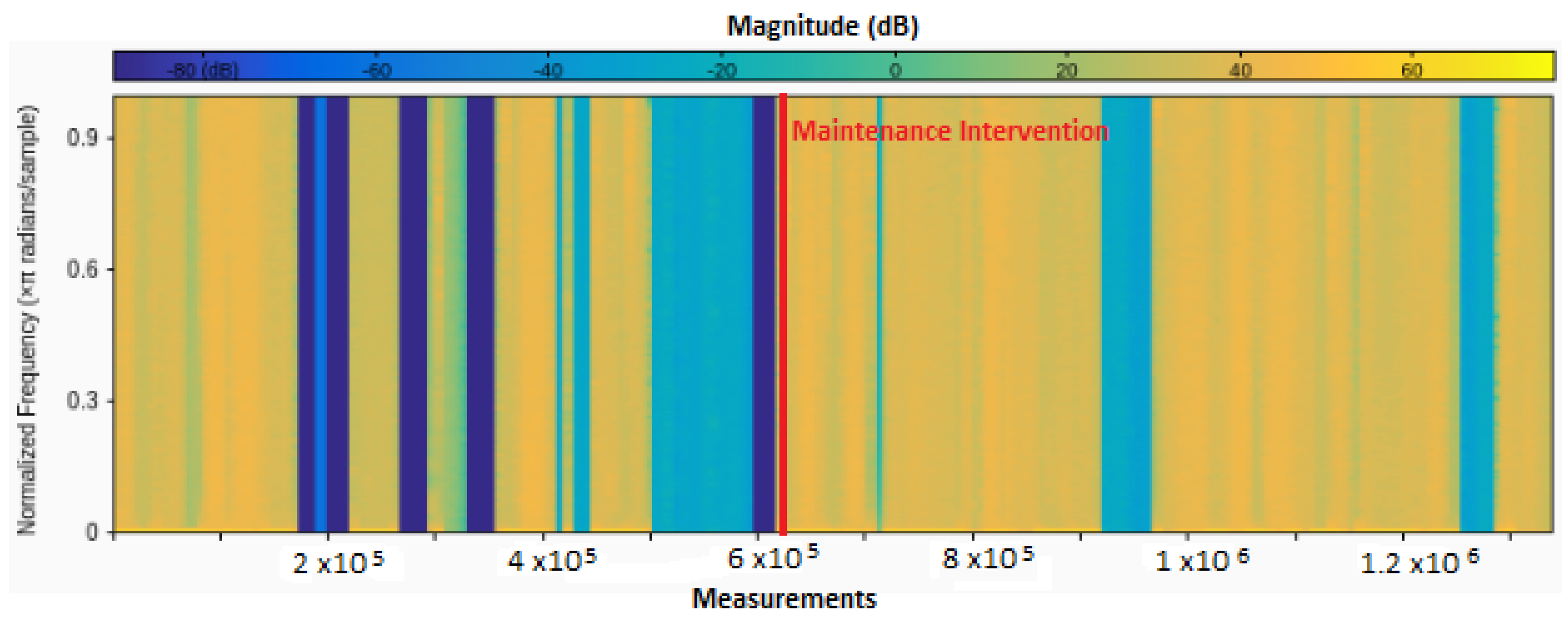
In our experimental scenario, we applied a STFT to each sensor signal with a Hann window of size 128 and 50% of overlapping. After that, we found that some periods with the fewer magnitude frequencies appeared could be related with CUs degradation. In
Figure 2, in which the SFTF of sensor
wqgsfv* corresponding to the
is illustrated, we observed that some of these (blue) periods appeared just before a maintenance intervention (vertical red line).
5.2. Hilbert Spectrum
After noticing that degradation of CUs may be related to the presence of periods with fewer magnitude frequencies, we were interested in using a time-frequency representation capable to catch those periods.
The Hilbert spectrum, defined by Equation (
3), is a time-frequency distribution of signal amplitude that helps in distinguishing a mixture of moving signals [
18]. The given spectrum is computed by: (1) mathematically decomposing a signal into Intrinsic Mode Functions (IMF); and (2) applying the Hilbert transform to compute the instantaneous frequency of each component by obtaining
(the derivative of the phase
w.r.t the time
t) [
13]. After performing the Hilbert transform on
n IMF signals, the Hilbert spectrum is obtained. In practice, the Hilbert-Huang transform (HHT) has been widely used to obtain
[
13]:
where
represents the real part of terms within brackets and both
and
are constants.
This transform uses the Empirical Model Decomposition (EMD) to get the IMF signals, for then, apply the Hilbert transform to each signal. Despite the implementation of the EMD depends on how IMFs are defined and the stop criterion used to find them [
19], the implemented through a sifting process is composed of the following steps:
Identify all the local extrema of the input signal .
Separately connect all the maxima and minima with natural cubic spline lines to form the upper, , and lower, , envelopes.
Compute the mean of the envelopes as .
Find a tentative IMF as the difference between the and , .
Check if satisfy the IMF definition and stoppage criterion.
If does not satisfy the definition, repeat steps [1–5] many times til it satisfies the definition.
If does satisfy the definition, assign the tentative IMF as an IMF component, .
Repeat steps [1–7] on the residue, , as the data.
Stop when the residue contains no more than one extremum.
5.3. Physics Model-Based Approach
Our proposed approach, based on Hilbert spectrum modeling, aims to emphasize the periods in which sensor signals experience the lowest frequencies. Our approach constructs a single HI form each sensor signal
of a determined CU. In [
38], this procedure aims to capture the physics of the failure.
In the construction of the Hilbert spectrum, the accumulation of periods with similar frequencies is proposed by using IMFs. We are interested on the first IMF because it identifies and decomposes the finest component of the shortest period at each instant [
27].
To perform the EMD, the following definition of Intrinsic Mode Function was adopted:
IMF:any function having the same numbers (or at most differing by one) of zero-crossings and extrema, and also having symmetric envelopes defined by local maxima and minima, respectively [
19].
To get the first IMF
, the following mathematical operations are performed:
where indices refer an iteration
k of each EMD step. In our case, the EMD applied to get the first IMF
. In this implementation,
k iterations are performed while the difference
or while
does not satisfy the IMF definition. In this implementation,
, defined by Equation (4), is defined by the Cauchy type criterion [
13].
Once
is obtained from a single
time series, the
signal that corresponds to the evolution of health conditions is defined in Equation (5):
Given that the application of the integral operator implies obtaining large values, we performed a Z-score normalization process to the signal. The same normalization procedure was applied to the altitude, the airspeed and the flight phase to use them as inputs for the following technical processes.
6. Health Stage Division
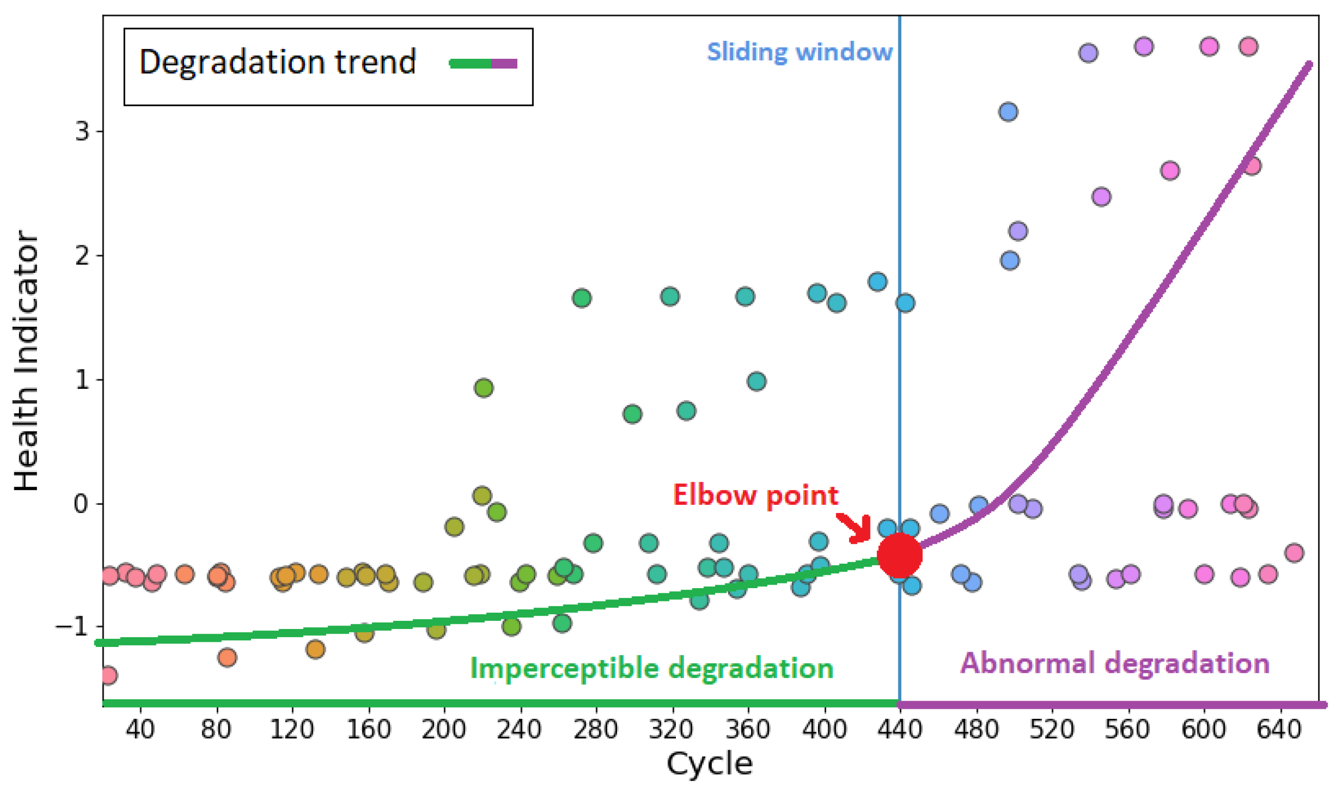
Once Health Indicators were obtained, we considered using two health stages proposed in [
11,
17,
34]. That consideration, illustrated in
Figure 3, implies that CUs experience an imperceptible degradation before experiencing a abnormal degradation [
8,
11]. In that sense, the following piecewise function, defined by Equation (
6), was formulated to identify the point (
elbow point) that separates both degradation stages by conducting a binary classification. In Equation (
6), a measurement labeled with 0 means that it corresponds to the imperceptible degradation, otherwise, it corresponds to the abnormal degradation stage.
Although statistical procedures such as t-test have been applied to identify the
elbow point (red point), we adopted ML algorithms used in [
17], since they have provided an accurate distinction between health degradation stages. Note that the lengths of imperceptible and abnormal degradation stages can have a large number of combinations, as in
Figure 3. For that reason, a sliding window (blue vertical line) technique has been adopted to identify the best partition.
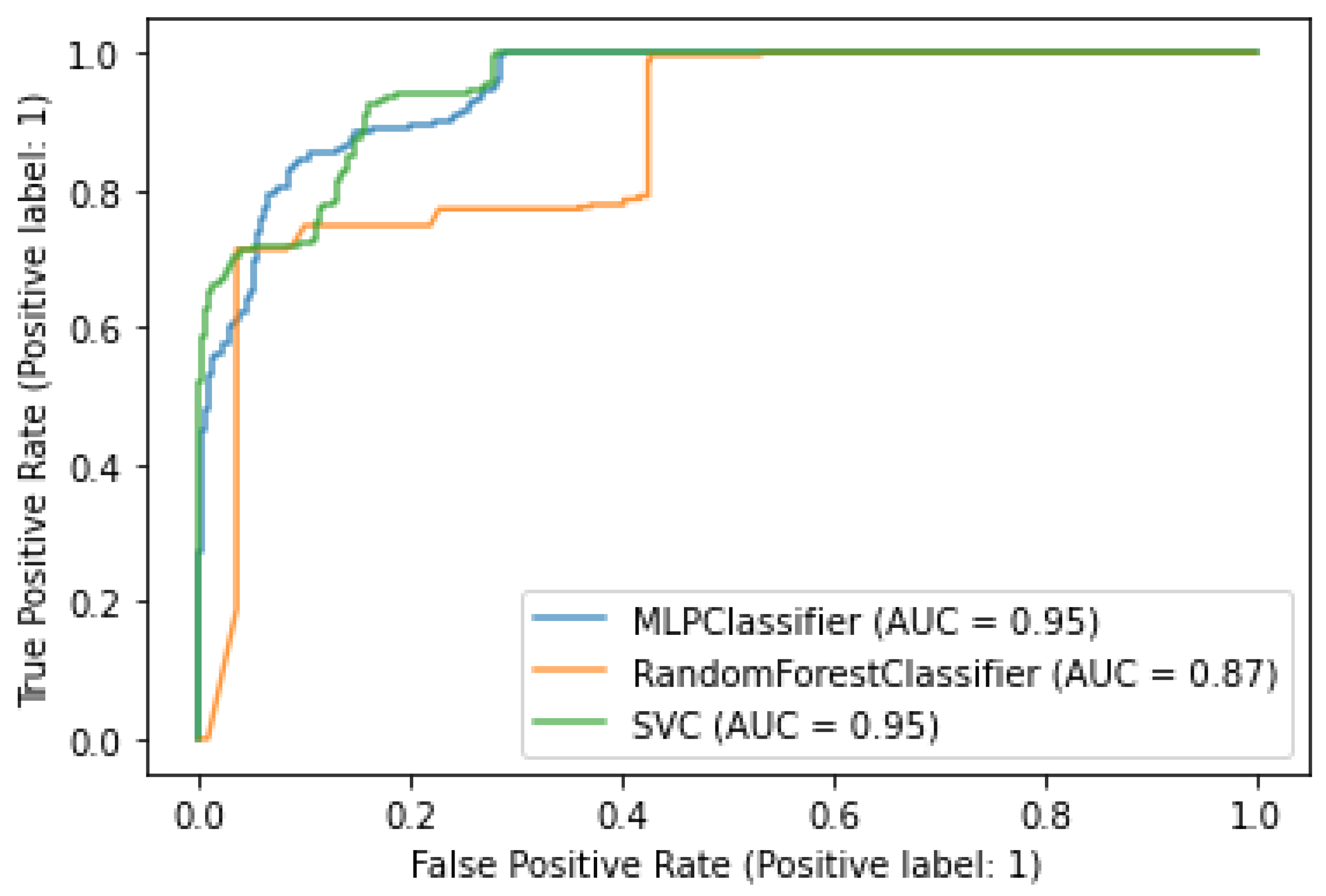
Because in [
17], the classification health stages has obtained promising results using CMAPSS data and the following algorithms: Multi-Later Perceptron (MLP), Random Forest Classifier (RFC) and Support Vector Classifier (SVC), we used them to distinguish the two health stages (0: imperceptible and 1: abnormal). The underlined configuration settings for these algorithms were selected by evaluating the hyperparameters detailed in
Table 2.
Once hyperparameter tuning was conducted by fixing the elbow point into the last 48 flight hours, the parameters in bold were selected when models presented the higher classification performance. In
Figure 4, we observe that those hyperparameters were selected when the classifiers obtained the higher values for the Area Under the Curve (AUC).
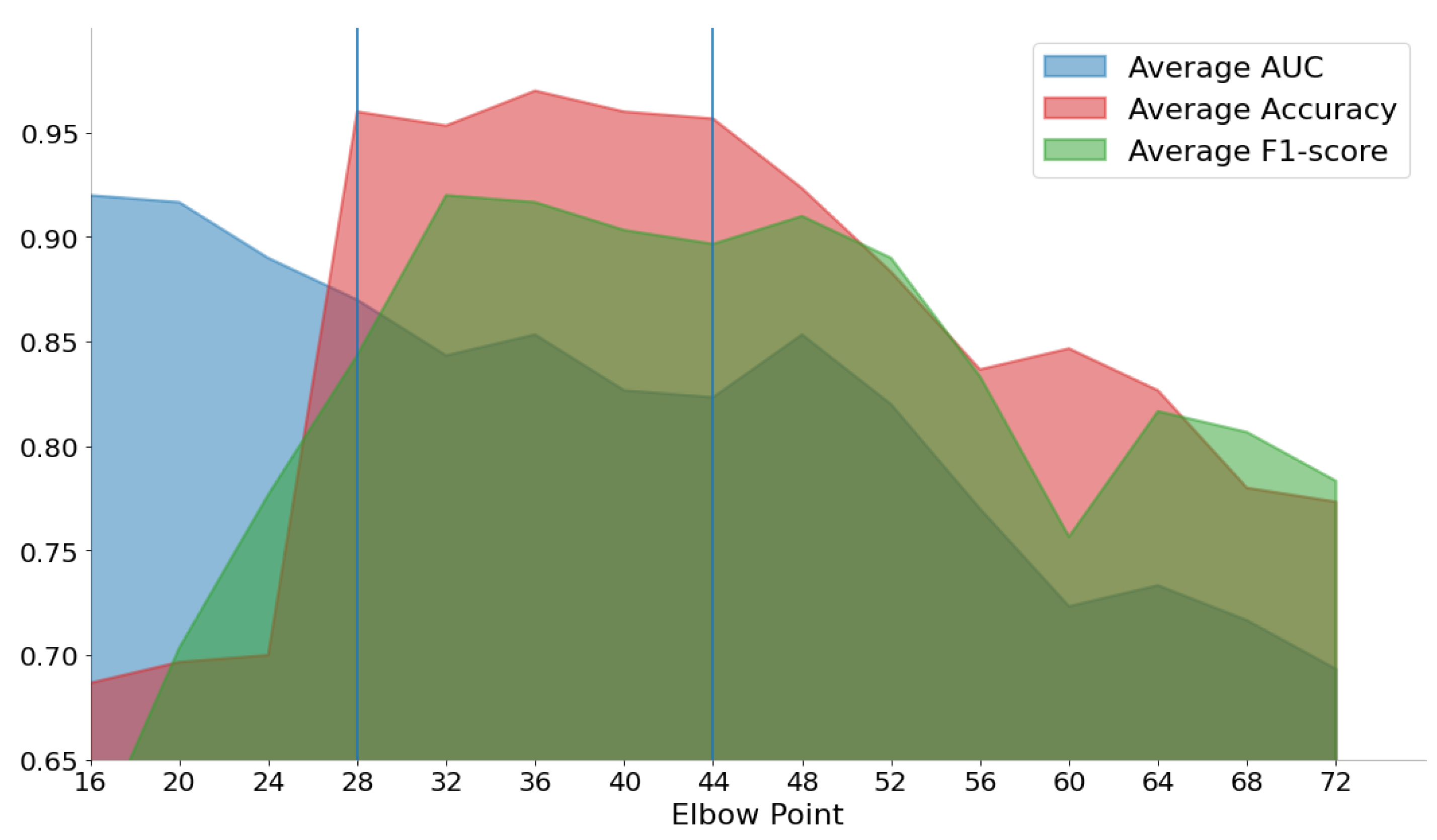
To identify the point that better separates the health stages, we used a window of 4 flight hours. In
Table 3, we observed that the elbow point took values from 16 to 72 with a step size of 4. After comparing the classification performance of models trained with different elbow point, we identified the best classifications when that point is configured between the last 28 and 44 flight hours.
Since we are comparing the performance of groups of three classifiers (RFC, SVC and MLP), we averaged their accuracy, F1-score and AUC to used it as comparison criterion. We used the average Accuracy as a selection criterion to highlight the period in which classification takes the best performances. In
Figure 5, in which the average of classification metrics is illustrated for different elbow point values, we see that the best classifications were achieved when that point takes a value from 44 to the last 28 flight hours.
7. RUL Estimation
Predictive maintenance aims to estimate the equipment lifetime, usually since it started to be monitored. Detecting an abnormal degradation stage when a aircraft achieves its 44 last operating hours gives technicians time to minimize Aircraft On Ground (AOG) times. The worst-case could be detecting the abnormal degradation when the system is very close to failing. According to our piecewise degradation function, defined by Equation (
7), large values for the elbow point are preferred in our case. While the imperceptible degradation stage takes a RUL equal to the elbow point, the abnormal degradation stage takes a RUL similar to Equation (
1), where the floor and ceiling operators are limited to RUL
. To use this signal as input for the ML algorithm, its range was also reduced using the Z-score normalization process.
A multi-layer perceptron algorithm demonstrated to be useful to estimate the RUL. From the list of hyperparameters detailed in
Table 4, the options in bold were demonstrated to reduce the estimation error.
The loss function used to train the model and evaluate its achieved performance corresponds to the Root Mean Squared Error (RMSE) metric:
where,
m is the number of measurements, RUL is the ground truth for the measure
i and
is the remaining useful life inferred. Given that the sampling rate of 1 Hz in data collection implies the analysis of a large
m, we considered evaluating four downsampling rate configurations, namely:
Hz,
Hz,
Hz and
Hz.
Our experiments demonstrate that a down sampling rate of Hz is able to significantly reduce the time on the training process and the estimation error. We conclude that after obtaining 10 models by fixing the elbow point at 44, and then, calculating the mean and the standard deviation for the RMSE. The best performance was achiever by the down sampling rate Hz, which obtained a RMSE of 9.99 ± 1.29, while the other down sampling rates presented significant larger performances.
Implementing an early stopping strategy to prevent overfitting and reduce the training time, we were able to train the RUL prediction model in less than 2 min. That strategy considered training the model with a maximum of 580 epochs and evaluating the minimization on the loss function at 10 epochs.
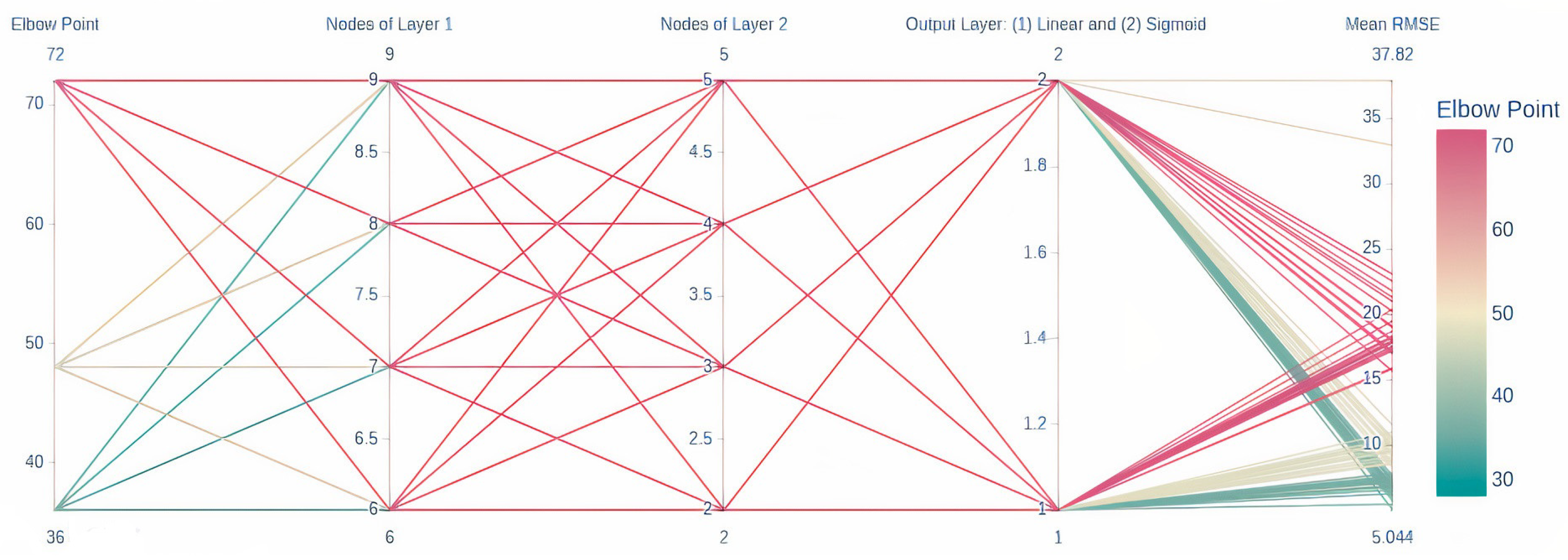
After configuring the early stopping strategy and defining an adequate down sampling rate, we evaluated the influence of the elbow point, the number of nodes of hidden layers and the activation function used in the output layer. In
Figure 6, we can observe that the elbow point and the activation function (0: sigmoid and 1: linear) really compromise the estimation error. For each combination of the factors analyzed, 10 models were obtained to evaluate them by comparing confidence intervals.
We considered evaluating three values for the elbow point, namely: 72, 48, and 36. Those values correspond to the assumptions that the variance of failures may be predicted 3, 2 and 1.5 operating days before experiencing a critical failure. In
Figure 6, we can observe that RUL predictions are accurate when elbow point is set into the last operating flight hours. Predicting the health status into a large failure degradation implies increasing the estimation error. However, there are cases in which early predictions are preferred.
Observing the influence of the activation function of the output layer, we are able to notice that the linear activation function on the output layer aims to present accurate results. At the other hand, observing the influence of number of nodes of the layers, we were able to identify the more accurate predictions when the first and second hidden layers have 7 and 4 nodes, respectively.
8. Results and Discussion
The PHM program described in
Section 3 has illustrated the construction path of physics-based and data-driven approaches. In case of data transformations from time or frequency domains not being appropriate to identify health degradation patterns directly from data, our PHM program suggests constructing physics-based Health Indicators and using them as inputs of data-driven approaches.
To evaluate the performance gaining by construction the time-frequency HIs with the proposed approach, we decided to train RUL estimators using raw data and using the HIs. In
Table 5, we observe the performance obtained with three different elbow points. Recall that the health stage division allowed the construction of a piece-wise degradation, in which the RUL lineally decrease into the last flight hours. The elbow points presented in
Table 5 correspond to the points that better divided the proposed two health stages.
To choose the better elbow point, we calculated the mean and the standard deviation of the RMSE after getting 10 RUL predictors per point. All the models were trained using the same downsampling rate, degradation function, Z-score normalization, MLP hyperparameters and early stopping settings, but differing in input data. Results presented fewer prediction errors by setting a linear degradation within the last 48 flight hours.
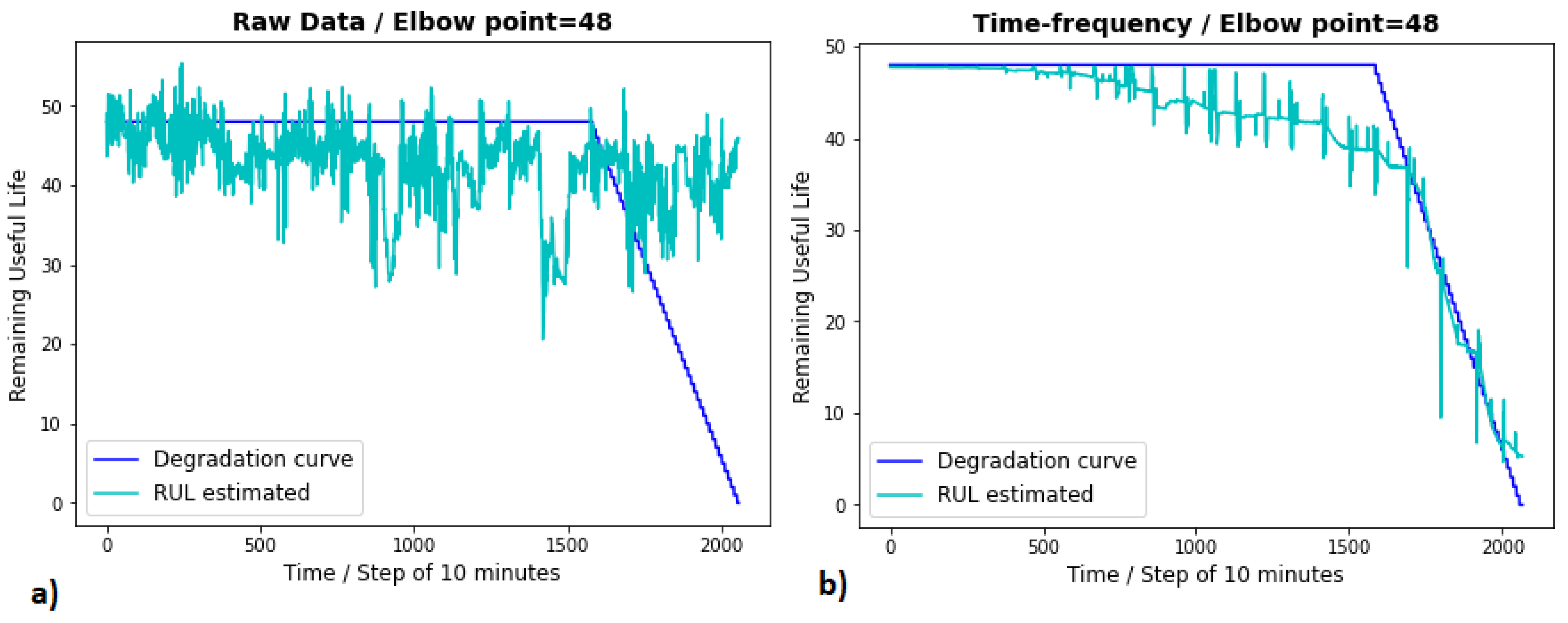
In
Figure 7, the RUL estimation of the first CU of the aircraft
enwslczm is compared by using different input, namely: (a) raw data and (b) HIs constructed from the time-frequency domain. In (a), we can observe that the RUL estimated curve (light blue curve) oscillates around the value defined in the imperceptible health stage (blue curve). However, fails in predicting the RUL in the abnormal health stage. On the other hand, in (b), the HI construction seems to solve that problem because the RUL estimated curve (light blue curve) follows a similar tendency into the last flight hours.
Comparing the results of applying HI construction versus using raw data trained with an elbow point of 48, we notice that (b) improved the predictions of (b). While the raw data approach obtained a RMSE of , the HI construction obtained a RMSE of . These performance gains are mainly related to RUL estimations on the abnormal degradation stage, where the estimations of (b) are closer to the proposed degradation curve than (a).
9. Conclusions and Future Work
The Health Indicators constructed from the time-frequency domain were demonstrated to be useful to describe the degradation of the cooling units of the wide body aircraft. The construction of HIs was not only useful to predict the Remaining Useful Life of aerial subsystems, but was also useful to identify two health stages of CUs, namely: an imperceptible degradation stage and a abnormal degradation stage.
After estimating the RUL of aerial systems, we believe that our HI construction approach could be used when machinery degradation may be related to the presence of periods with the lowest power spectrum. In general, we believe that our work can be easily replicated. While our HI construction approach applies the well-known Empirical Mode Decomposition (EMD) method used to obtain Intrinsic Mode Functions (IMFs), our prognostics program should be adopted in the presence of stationary and non-stationary signals. Before reusing our approach in other PHM applications, we recall that is important to evaluate the development of physics-based and data-driven models separately. The development of hybrid approaches is recommended when individual approaches do not satisfy the PMH practitioner’s expectations. In the near future, we are interested in providing our estimations to aerospace maintenance technicians in order to evaluate the potential of our approach in practice.
Author Contributions
Conceptualization, R.L.R., C.S. and B.R.; methodology, R.L.R.; software, R.L.R.; validation, R.L.R., C.S. and B.R.; formal analysis, C.S.; investigation, R.L.R.; resources, R.L.R., C.S. and B.R.; data curation, R.L.R.; writing—original draft preparation, R.L.R.; writing—review and editing, R.L.R., C.S. and B.R.; visualization, R.L.R.; supervision, C.S. and B.R. All authors have read and agreed to the published version of the manuscript.
Funding
This work was partially supported by: (1) The Portuguese Foundation for Science and Technology (FCT) under the project grant SFRH/BD/07344/2020, and (2) The European Union’s Horizon 2020 research and innovation programme under the project No 769288 untitled “Real-Time Condition-based Maintenance for Adaptive Maintenance Planning-ReMAP”.
Acknowledgments
The data analyzed in this paper is part of the ReMAP project.
Conflicts of Interest
The authors declare no conflict of interest.
Abbreviations
The following abbreviations are used in this manuscript:
| AI | Artificial Intelligence |
| CBM | Condition-Based Maintenance |
| CM | Condition Monitoring |
| CS | Cooling System |
| CU | Cooling Unit |
| EMD | Empirical Mode Decomposition |
| FF | Fast-Fourier |
| HI | Health Indicator |
| IMF | Intrinsic Mode Function |
| ML | Machine Learning |
| MLP | Multi-Layer Perceptron |
| PHM | Prognostics and Health Maintenance |
| PM | Predictive Maintenance |
| RFC | Random Forest Classifier |
| RUL | Remaining Useful Life |
| STFT | Short-Time Fourier Transform |
| SVC | Support Vector Classifier |
| WVD | Wigner-Ville Distribution |
References
- Basora, L.; Bry, P.; Olive, X.; Freeman, F. Aircraft Fleet Health Monitoring with Anomaly Detection Techniques. Aerospace 2021, 8, 103. [Google Scholar] [CrossRef]
- Chen, X.; Yu, J.; Tang, D.; Wang, Y. Remaining useful life prognostic estimation for aircraft subsystems or components: A review. In Proceedings of the 10th International Conference on Electronic Measurement and Instruments, Chengdu, China, 16–19 August 2011. [Google Scholar]
- Adhikari, P.; Rao, H.G.; Buderath, M. Machine Learning based Data Driven Diagnostics & Prognostics Framework for Aircraft Predictive Maintenance. In Proceedings of the 10th International Symposium on NDT in Aerospace, Dresden, Germany, 24–26 October 2018. [Google Scholar]
- Javed, K.; Gouriveau, R.; Zemouri, R.; Zerhouni, N. Features Selection Procedure for Prognostics: An Approach Based on Predictability. IFAC Proc. Vol. 2012, 45, 25–30. [Google Scholar] [CrossRef] [Green Version]
- Patrick, R.; Smith, M.; Zhang, B.; Byington, C.; Vachtsevanos, G.; Del Rosario, R. Diagnostic enhancements for air vehicle HUMS to increase prognostic system effectiveness. In Proceedings of the 2009 IEEE Aerospace Conference, Big Sky, MT, USA, 7–14 March 2009. [Google Scholar]
- Atamuradov, V.; Medjaher, K.; Dersin, P.; Lamoureux, B. Prognostics and Health Management for Maintenance Practitioners-Review, Implementation and Tools Evaluation. Int. J. Progn. Health Manag. 2017, 12, 31–62. [Google Scholar] [CrossRef]
- Biggio, L.; Kastanis, I. Prognostics and Health Management of Industrial Assets: Current Progress and Road Ahead. Front. Artif. Intell. 2020, 3, 88. [Google Scholar] [CrossRef] [PubMed]
- Saxena, A.; Celaya, J.; Balaban, E.; Goebel, K.; Saha, B.; Saha, S.; Schwabacher, M. Metrics for evaluating performance of prognostic techniques. In Proceedings of the International Conference on Prognostics and Health Management, Denver, CO, USA, 6–9 October 2008. [Google Scholar]
- Jones, D.; Snider, C.; Nassehi, A.; Yon, J.; Hicks, B. Characterising the Digital Twin: A systematic literature review. CIRP J. Manuf. Sci. Technol. 2020, 29, 36–52. [Google Scholar] [CrossRef]
- Titchmarsh, E.C. Introduction to the Theory of Fourier Integrals; Oxford University Press: Oxford, UK, 1938; Volume 141, p. 183. [Google Scholar]
- Arias C., M.; Kulkarni, C.; Goebel, K.; Fink, O. Aircraft Engine Run-to-Failure Dataset under Real Flight Conditions for Prognostics and Diagnostics. Data 2021, 6, 5. [Google Scholar] [CrossRef]
- Kan, M.S.; Tan, A.C.C.; Mathew, J. A review on prognostic techniques for non-stationary and non-linear rotating systems. Eur. J. Oper. Res. 2015, 62–63, 1–20. [Google Scholar] [CrossRef]
- Huang, N.E.; Zheng, S.; Steven, R.; Manli, C.W.; Hsing, H.S.; Quanan, Z.; Nai-Chyuan, Y.; Chi, C.T.; Liu, H.H. The Empirical Mode Decomposition and the Hilbert Spectrum for Nonlinear and Non-Stationary Time Series Analysis. Proc. R. Soc. London Ser. A Math. Phys. Eng. Sci. 1971, 03, 903–995. [Google Scholar] [CrossRef]
- Matz, G.; Hlawatsch, F. Wigner distributions (nearly) everywhere: Time-frequency analysis of signals, systems, random processes, signal spaces, and frames. Signal Process. 2003, 83, 1355–1378. [Google Scholar] [CrossRef]
- Lei, Y.; Li, N.; Guo, L.; Li, N.; Yan, T.; Lin, J. Machinery health prognostics: A systematic review from data acquisition to RUL prediction. Mech. Syst. Signal Process. 2018, 104, 799–834. [Google Scholar] [CrossRef]
- Azevedo, D.; Cardoso, A.; Ribeiro, B. Estimation of Health Indicators using Advanced Analytics for Prediction of Aircraft Systems Remaining Useful Lifetime. Int. J. Progn. Health Manag. 2020, 5, 1–10. [Google Scholar]
- Baptista, M.L.; Henriques, E.M.P.; Goebel, K. More effective prognostics with elbow point detection and deep learning. Mech. Syst. Signal Process. 2021, 146, 106987. [Google Scholar] [CrossRef]
- David, H. Grundzüge einer allgemeinen Theorie der linearen Integralgleichungen. In Integralgleichungen und Gleichungen mit unendlich vielen Unbekannten; Vieweg + Teubner Verlag, Ed.; Publishing House: Wiesbaden, Germany, 1989; pp. 8–171. [Google Scholar]
- Wang, G.; Chen, X.; Qiao, F.; Wu, Z.; Huang, N.E. On Intrinsic Mode Function. Adv. Adapt. Data Anal. 2011, 2, 277–293. [Google Scholar] [CrossRef]
- Jardine, A.K.S.; Lin, D.; Banjevi, D. A review on machinery diagnostics and prognostics implementing condition-based maintenance. Mech. Syst. Signal Process. 2006, 20, 1483–1510. [Google Scholar] [CrossRef]
- Sikorskaab, J.Z.; Hodkiewiczb, M.; Ma, L. Prognostic modelling options for remaining useful life estimation by industry. Mech. Syst. Signal Process. 2011, 25, 1803–1836. [Google Scholar] [CrossRef]
- Si, X.S.; Wang, W.; Hua, C.H.; Zhou, D.H. Remaining useful life estimation—A review on the statistical data driven approaches. Eur. J. Oper. Res. 2011, 16, 1–14. [Google Scholar] [CrossRef]
- Basora, L.; Olive, J.; Dubot, T. Recent Advances in Anomaly Detection Methods Applied to Aviation. Aerospace 2019, 6, 117. [Google Scholar] [CrossRef] [Green Version]
- Heng, A.; Zhang, S.; Tan, C.C.A.; Mathew, J. Rotating machinery prognostics: State of the art, challenges and opportunities. Mech. Syst. Signal Process. 2009, 23, 724–739. [Google Scholar] [CrossRef]
- Bieber, M.; Verhagen, W.J.C.; Santos, B.F. An Adaptive Framework for Remaining Useful Life Predictions of Aircraft Systems. Int. J. Progn. Health Manag. 2021, 6, 60–70. [Google Scholar]
- Tracer, B.; Loughlin, P.J. What are the time-frequency moments of a signal? In Proceedings of the International Conference on Acoustics, Speech, and Signal Processing Conference Proceedings, Atlanta, GA, USA, 9 May 1996. [Google Scholar]
- Seif, H.; Duff, L.; Guy, P.; Laurent, S.; Rachid, G.; Ghozlen, H.B.M. Hilbert-Huang Transform versus Fourier Based Analysis for Diffused Ultrasonic Waves Structural Health Monitoring in Polymer Based Composite Materials. PU-S05: Structural Health Monitoring. 2012, 1, 2417–2422. [Google Scholar]
- Zhang, B.; Zhang, L.; Xu, J. Degradation Feature Selection for Remaining Useful Life Prediction of Rolling Element Bearings. Qual. Reliab. Eng. Int. 2015, 32, 547–554. [Google Scholar] [CrossRef]
- Scott, A.C. Nonlinear Biology; Springer: Berlin/Heidelberg, Germany, 2007; pp. 181–276. [Google Scholar]
- Cao, J.-L.; Chen, G.-H. Introduction to the Theory of Fourier Integrals. Shanghai Univ. 2003, 7, 265–269. [Google Scholar] [CrossRef]
- Khalil, S.; Khalil, T.; Nasreen, S. A Survey Of Feature Selection And Feature Extraction Techniques In Machine Learning. In Proceedings of the Science and Information Conference, London, UK, 27–29 August 2014. [Google Scholar]
- Hu, Z.; Baoa, Y.; Xionga, T.; Chiongb, R. Hybrid filter–wrapper feature selection for short-term load forecasting. Eng. Appl. Artif. Intell. 2015, 40, 17–27. [Google Scholar] [CrossRef]
- H2020 Remap. Available online: https://h2020-remap.eu/ (accessed on 3 March 2022).
- Llasag Rosero, R.; Silva, C.; Ribeiro, B. Remaining Useful Life Estimation in Aircraft Components with Federated Learning. Int. J. Progn. Health Manag. 2020, 5, 1–9. [Google Scholar]
- Li, X.; Ding, Q.; Sun, J.Q. Remaining Useful Life Estimation in Prognostics Using Deep Convolution Neural Networks. Reliab. Eng. Syst. Saf. 2018, 172, 88. [Google Scholar] [CrossRef] [Green Version]
- Nguyen, T.P.K.; Amor, K.; Medjaher, K.; Picot, A.; Maussion, P.; Tobon, D.; Chauchat, B.; Cheron, R. Analysis and comparison of multiple features for fault detection and prognostic in ball bearings. Int. J. Progn. Health Manag. 2018, 4, 1. [Google Scholar]
- Kehtarnavaz Nasser, L. DSP System Design: Cochlear Implant Simulator. In Digital Signal Processing System Design, 2nd ed.; Academic Press: Burlington, VT, USA, 2008; pp. 303–320. Available online: https://www.sciencedirect.com/book/9780123744906/digital-signal-processing-system-design (accessed on 3 March 2022).
- Hu, C.; Youn, B.D.; Wang, P.; Joung, T.Y. Ensemble of data-driven prognostic algorithms for robust prediction of remaining useful life. Reliab. Eng. Syst. Saf. 2012, 103, 120–135. [Google Scholar] [CrossRef] [Green Version]
| Publisher’s Note: MDPI stays neutral with regard to jurisdictional claims in published maps and institutional affiliations. |
© 2022 by the authors. Licensee MDPI, Basel, Switzerland. This article is an open access article distributed under the terms and conditions of the Creative Commons Attribution (CC BY) license (https://creativecommons.org/licenses/by/4.0/).


