1. Introduction
With the rapid development of the civil aviation industry, air transport demand continues to grow rapidly. However, limited airspace resources and the slow progress of air traffic control technologies cannot meet the rapidly increasing demand for transportation, resulting in increasingly crowded airspace. Airspace congestion can lead to a series of problems, such as flow control, flight delays (increased potential flight conflicts, reduced flight safety), and longer flight times (increase pollutant emissions). In the face of airspace congestion, identifying air traffic congestion is the premise and foundation of air traffic management [
1].
Currently, the air traffic management mode adopts an operation mode based on the air traffic control sector (ATCS). The airspace divides into multiple sectors with relatively fixed boundaries. Air traffic controller management is responsible for the orderly transfer of aircraft into and out of the sector and guides the aircraft to fly safely within the controlled sector [
2,
3]. This paper aims to identify the degree of ATCS congestion, which has strategic and tactical significance. Strategically, recognizing the historical congestion of a sector can provide a basis for decision-making on sector consolidation and addition. Tactically, real-time recognition of each sector’s congestion allows controllers to dynamically grasp the congestion status of the sector and neighboring sectors, which allows them to more effectively guide the aircraft through this sector and reasonably hand it over to adjacent sectors.
ATCS congestion recognition is also known as complexity assessment [
4,
5]. Many researchers have studied sector congestion recognition and improved methods using two aspects: evaluation indicators and evaluation methods. In terms of the construction of congestion evaluation indicators, current research mainly considers the reasons for congestion, the workload of controllers, and the characteristics of congestion. To construct indicators from the perspective of congestion causes, we mainly consider the imbalance between traffic demand and traffic capacity. Wanke et al. [
6] quantified the uncertainty of predicted flow level and airspace capacity, and then solved the probabilistic model of traffic demand prediction. At the same time, they obtained a monitor for predicting the probability of a congestion alarm. Subsequently, Mulgund et al. [
7] applied a genetic algorithm to airspace structure management in 2006, easing the degree of air traffic congestion through two solutions: reprogramming of flight tracks and flight delays on the ground. Sood et al. [
8] went a step further. They developed adaptive genetic algorithms based on weather factors and traffic predictions to balance multiple metrics, which was different from traditional viewing genetic algorithms, and simulated its results.
Since the controller manages each sector, the controller’s workload directly reflects the sector’s congestion. Some studies have constructed congestion metrics from the controller’s workload perspective. Djokic et al. [
9] proposed the conjecture that there might be a connection between the communication load and the controller’s load according to the execution process of the controller’s work. They proved the conjecture through principal component analysis of many parameters related to aircraft, followed by step-by-step multiple regression analysis. Van Paassen et al. [
10] established an airspace complexity indicator system and evaluated the complexity based on the characteristic quantity in the process of aircraft conflict relief. On the other hand, input-output flow is also an important indicator to reflect the degree of congestion. Lee et al. [
11] constructed an input-output system framework to analyze the airspace and expressed the airspace complexity in a given traffic situation using a complex graph. Then, on the original basis, the disturbance to the closed system was considered, that is, the change of airspace complexity when the system enters the aircraft, and how the air traffic controllers respond to it. Additionally, Laudeman et al. [
12] proposed the concept of spatial dynamic density. Based on the existing assessment methods of traffic density, combined with traffic complexity, the indicator of traffic complexity was determined, and a dynamic density equation was constructed to measure the workload of traffic controllers. Kopardekar et al. [
13], based on their predecessors, researched the city of Cleveland and constructed a measurement matrix of dynamic density, they then used code reduction and analysis tools to simulate the aircraft in the sector in real-time, thereby simulating the load of the controller. In addition, some researchers have combined the selection of evaluation indicators with machine learning. Chatterji and Sridhar [
14] divided the constructed evaluation indicators of air traffic complexity into ten sets for neural network training to select the best set for evaluating controller workload performance.
In addition to the characterization of congestion behaviors from the causes and controller’s workload, researchers have also constructed congestion indicators from the characteristics of congestion. Delahaye and Puechmorel [
15] divided the air traffic congestion indicator into two parts based on the complexity indicator constructed by predecessors. One is the aircraft geometry attribute; the other uses the expression of air traffic flow as a dynamic system to obtain the complexity measurement index through topological entropy. Further, Delahaye et al. [
16] carried out the nonlinear expansion of the linear dynamic system, calculated its related Lyapunov index, and obtained the complexity, which can be used to identify the high (or low) complexity regions on the map. Lee et al. [
17], based on the nonlinear dynamic system, incorporated the uncertainty of flight trajectory into the spatial dynamical system’s construction process and improved the original system.
Another challenging issue is assessing the level of congestion. The present research can be divided into the threshold discrimination method, comprehensive weighting method, cluster analysis method, and machine learning method. Early studies were mainly based on threshold discrimination, comprehensive weighting, and cluster analysis. Bilimoria and Lee [
18] proposed an automatic cluster recognition method that uses the cluster quality indicator obtained from the threshold distance of aircraft to identify the crowding situation in the high-dynamic region. Surakitbanharn et al. [
19] proposed a linear weighting method to integrate congestion evaluation indicators. Because of the nonlinear relationship between the congestion indicators, the model precision was reduced by linear weighting. Brinton and Pledgie [
20] used the collection characteristics of aircraft action trajectories for clustering, constructed complexity indicators from the perspective of dynamic density, calculated airspace complexity, and partitioned its airspace. Nguyen [
21] segmented the aircraft trajectory, used a deterministic annealing algorithm for linear clustering, classified it according to time, and finally output the clustering result. Based on the complex network theory, Wang et al. [
22] divided the aviation network into 2D and 3D, established a two-layer and multi-level dynamic network model, and divided the complexity into three categories by using a clustering algorithm to discuss the change frequency of traffic conditions.
In recent years, machine learning methods have attracted researchers’ attention. Gianazza [
23] used principal component analysis to extract six key factors from 28 complexity indicators and used BPNN (Back Propagation neural network) to evaluate the crowding level of sectors. Xi et al. [
24] proposed an integrated learning model based on the complexity of air traffic in the region, considering that the cost of sample labeling is too high, which leads to the problem that the labeled samples are insufficient for training. Jiang et al. [
4] put forward a method for identifying sector congestion based on the independent component analysis. A sector congestion indicator system was established based on complex network theory. The independent component analysis method was used to analyze the main components of all discriminative indicators and extracted by detection. The main element of the indicator is the abnormal value of the actual sector operation to determine whether the sector’s operating status is abnormal.
The machine learning method mentioned above can achieve excellent results, but the prerequisite is based on having enough labeled samples. However, sample marking must be done by experienced controllers, requiring a lot of time and energy. Even if we obtain a large number of labeled samples, mainstream recognition methods, such as support vector machines (SVM) or shallow neural network models, cannot effectively capture the nonlinear relationship between overall congestion level and individual congestion evaluation indicators. Additionally, the traditional congestion indicators, such as the distance, density, and conflict times, are the results of the regulation of controllers. They cannot truly reflect the self-organizing behavior of aircraft. Due to the difference in the structure for each ATCS, the congestion characteristics vary from ATCS to ATCS. Therefore, it is necessary to construct indicators to measure congestion behavior from the mechanism of formation, thereby guaranteeing that the same indicator behaves consistently at the same congestion level in various ATCSs and is independent of spatial structure. So, the congestion recognition model is more general and suitable for the current mainstream ATCSs with fixed routes and the free route airspace partly used in Europe.
However, at present, most methods mainly use static structure and dynamic operation characteristics to characterize congestion, which leads to poor generalization and operability. In essence, ATCS is a complex network system composed of aircraft. The nodes in the network are aircraft, and the connections in the network are the interrelationships between aircraft. Thus, this paper transforms the problem of ATCS congestion recognition into the complexity of the aircraft state network system from the perspective of complexity theory. We propose the deep active learning (DAL) method for ATCS congestion recognition, which can achieve a relatively high recognition rate with the smallest labeled samples. The main contributions of this paper are as follows: (a) An aircraft state network is built from the perspective of complexity theory. Some complexity indicators are selected to characterize congestion according to the relationship between the aircraft status network and the actual operation of the control; (b) This paper adopts an iterative semi-supervised deep learning architecture, learns features from a small number of labeled samples and a large number of unlabeled samples through a sparse autoencoder, and builds a deep neural network model by stacking to improve the congestion recognition rate; (c) Least confidence, marginal sampling, and information entropy are introduced as metrics of sample selection. This method can choose samples that are significantly different from the features of the labeled sample set to reduce data redundancy and the cost of manually labeling.
The organization of this paper is as follows: In
Section 2, the problem of ATCS recognition is elaborated;
Section 3 proposes a deep active learning method to identify the degree of ATCS congestion, including how to use a sparse autoencoder to train hidden layer features, how to select representative samples from unlabeled samples, and the description of implementation steps. In
Section 4, the effectiveness and superiority of the model are verified through experiments. Finally,
Section 5 concludes this paper.
2. Problem Formulation and Method Overview
ATCS congestion recognition aims to classify the overall congestion of a sector according to multiple congestion characteristics. Suppose there are
evaluation indicators for sector congestion. Classify sector congestion level into
category, and the category label set is
, where
is the label for the
i-th class of congestion. Let
and
denote a feature vector composed of
indicator values and the congestion level at time
t. Identifying the sector congestion level can be regarded as a classification problem, that is, by training the classification model
, the feature vector
is mapped to the corresponding congestion level
:
As can be seen from (1), the problem of sector congestion recognition involves the construction of a suitable feature vector and a classification model . In response to this problem, there are three main challenges:
(a) Congestion evaluation indicators should be able to indirectly reflect the workload of the controller and have universal applicability and operability. Since sector congestion is ultimately reflected in the controller’s workload, if the congestion evaluation index cannot indirectly reflect the controller’s workload, the constructed index will not help improve the ability to identify congestion. To improve the generalization and practicability of the subsequent recognition model, the crowding index must have excellent crowding feature characterization capabilities and be easy to obtain from the monitoring information system.
(b) The congestion recognition model has the ability to characterize a large amount of training data. In general, the more training data, the better the model’s performance. However, shallow learning models (such as BPNN and SVM) have limited ability to capture features from data, and it is easy to saturate in performance. Entering more data does not improve model performance [
23,
24]. In contrast, for deep learning models, the more data involved in training, the more they can achieve their potential.
(c) The sample labeling strategy can reduce the redundancy of the labeled sample set. Usually, training a high-precision congestion recognition classifier requires a large number of labeled samples. The sector congestion level needs to be manually marked by an experienced controller, which is expensive. For example, every 10 s, sector status information will update. If one month of data is needed to train the classification model, the total number of samples is 259,200, which is labeled by a controller, six samples per minute, and 8 h of work a day, then it will take three months to mark them. In addition, if the data is not distinguished, some classes will be redundant, and some will be insufficiently labeled.
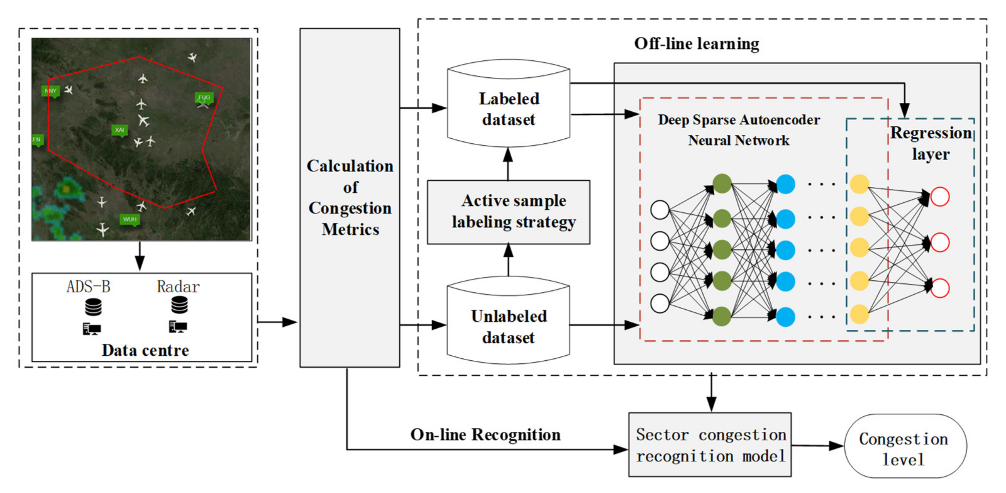
In response to the above three challenges, we transform sector congestion recognition into the complexity evaluation of aircraft state networks. This paper proposes a new sector congestion recognition architecture, as shown in
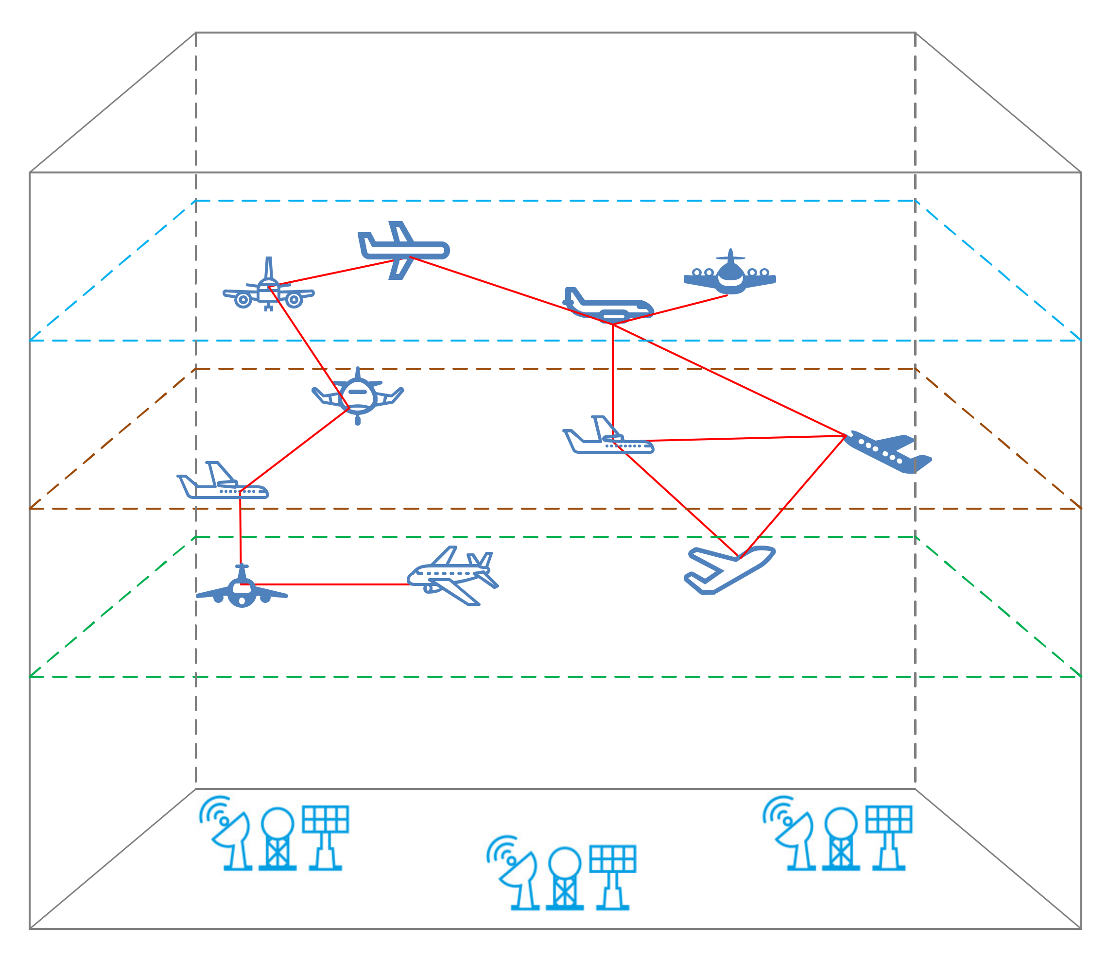
Figure 1. We first build a network with aircraft as nodes based on the aircraft’s dynamic trajectory and select appropriate complexity indicators to characterize sector congestion according to the aircraft’s self-organizing characteristics. The congestion indicators built in this way are not limited by the sector structure and are more universal. It is worth noting that the controller’s primary responsibility is to ensure the smooth passage of the aircraft without conflict. Therefore, the relationship between aircraft networks is determined according to the distance between aircraft and potential conflicts, which can ensure that the complexity index of aircraft networks can indirectly reflect the controller’s workload.
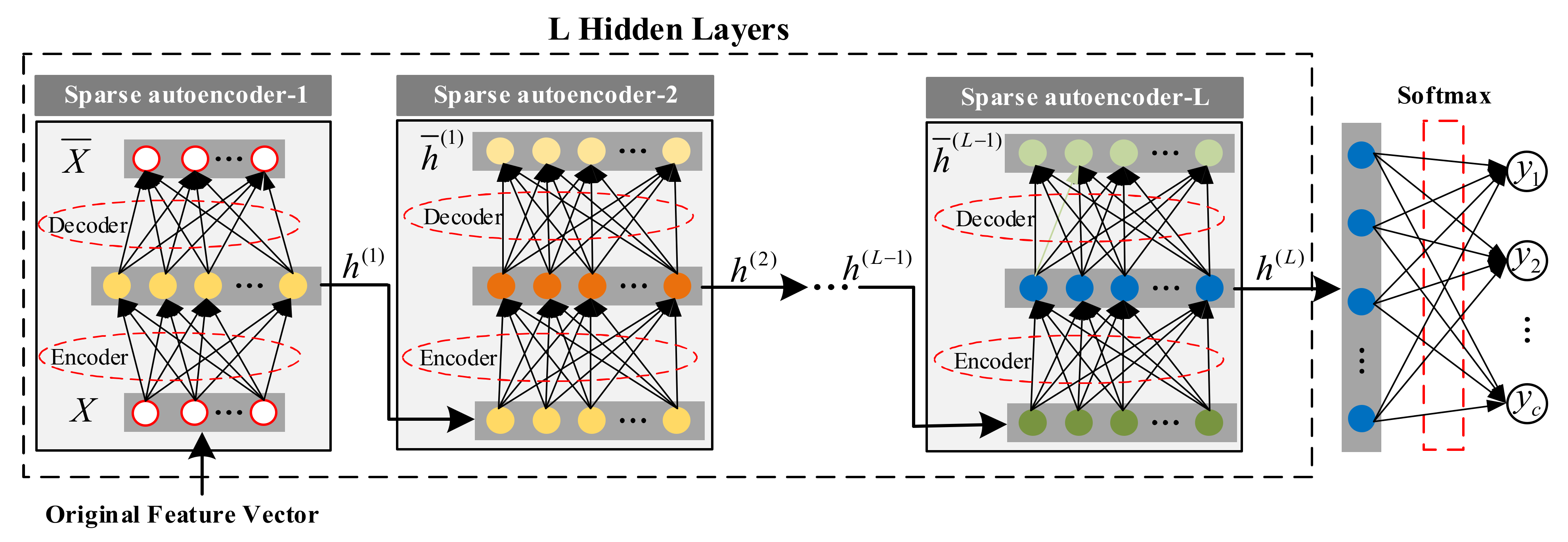
Based on the construction of indicators, we will establish a deep learning model to identify congestion. The model includes two modules, a classification model based on deep sparse auto-encoding and a sample labeling strategy. The model is trained offline using the idea of active learning. The classification model based on deep sparse auto-encoding is composed of hidden-layer sparse auto-encoding and output layer logistic regression. First, all data samples (labeled and unlabeled) are used to train the hidden layer parameters, and then the labeled sample set is used to fine-tune the model parameters. The model in this paper belongs to a type of deep neural network model, which can better characterize congestion features from a large amount of training data and improve the recognition rate. Simultaneously, according to certain selection principles, samples are selected from unlabeled samples for labeling to achieve the expected recognition rate with the least sample labeling. During the iterative process, the classification module and labeling strategy work together. Starting from the initial labeled training set, the model began to train the classification model based on deep sparse self-coding. The sample query strategy is adopted to select several samples from the unlabeled sample set. The classification model will be trained again after the newly labeled samples marked by controllers are added to the labeled sample set. The process is repeated until the model reaches the required performance.
4. Experimental Results and Analysis
This section verifies the validity and superiority of the method in this paper. First, the data used in the experiments and the model’s performance evaluation index are briefly introduced. Secondly, the optimal parameters select through experiments, and the sensitivity of the parameters is analyzed. Thirdly, the validity of the sample labeling strategy proposed in the model is verified. Finally, the effectiveness and superiority of our proposed model are confirmed by testing in multiple sectors and comparing it with mainstream methods.
4.1. Data
In the subsequent experiments of this paper, we selected three representative sectors for case analysis and marked them as “S1”, “S2”, and “S3” (as shown in
Figure 4). The experimental data selection period is from 1 September 2016 to 28 September 2016 6:00–24:00. Take 1 min as the time step to sample data. The total data collected by each sector are 30,240. Each piece of data contains attribute information such as flight number, longitude, latitude, and altitude. According to the calculation formula of the congestion evaluation indicators in
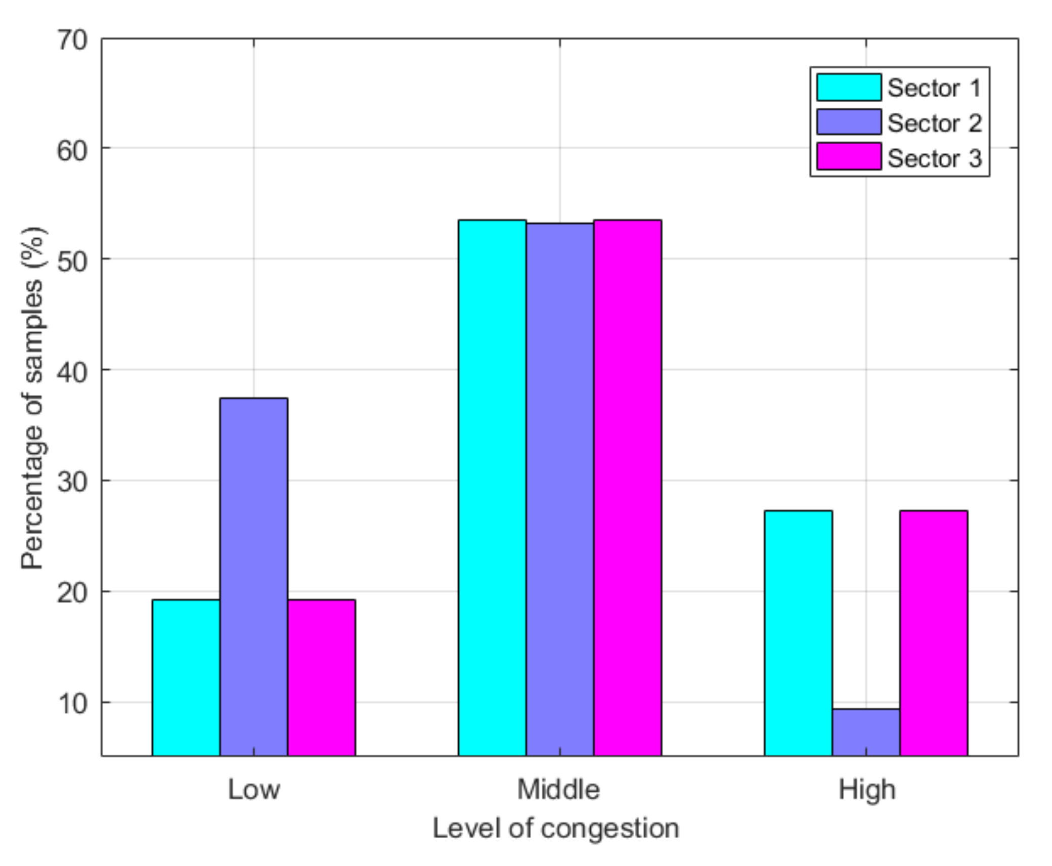
Section 2, we will obtain a sample set of experimental data. Each sample is represented by a 7-dimensional vector composed of the values of congestion indicators. After constructing the feature vectors of each sample, it is necessary to calibrate the samples’ congestion level. In the following experiments, we divide the congestion levels into three categories, which are represented by “1”, “2”, and “3”, which correspond to the three congestion levels of low, normal, and high, respectively. “1” and “2” are calibrated by air traffic controllers. To reduce the workload of the label and reduce the redundancy of labeled data, we use the process of active learning and use the sample selection method of basic information entropy. Each time, 300 samples are selected from the unlabeled sample set to mark the congestion level for 30 consecutive times. Each sector received 9000 labeled samples.
Figure 4 shows the proportion of each level. Further, from the labeled sample set, 7000 are randomly selected as the training set, and the remaining 2000 samples are used as the test set. Unlike mainstream supervised learning methods, this article belongs to a class of active learning methods. The training set includes 7000 labeled samples and 21,240 unlabeled samples.
4.2. Evaluation Metric
The proposed DAL method belongs to a class of iterative supervised learning classification methods. To this end, we use four evaluation measures: accuracy, precision, recall, and F-measure to evaluate the performance of the model. Accuracy is the percentage of correctly classified samples. Precision is the percentage of correctly classified samples in each class. The recall rate is the percentage of correctly classified samples in each category. The
combines accuracy and recall into one evaluation index. Let
denote the number of samples with the congestion degree of a class
being labeled as
, and
denote the number of samples with the congestion degree of a class
being labeled as
, where
. Each metric is defined as:
where
,
and
denote the precision, recall, and F-measure of the k-th class, respectively.
The four indices mentioned above reflect the performance of the model from different aspects. The accuracy rate reflects the overall situation of model performance. The evaluation is most effective when the number of samples is relatively uniform. It can be seen from
Figure 4 that the samples with “high” and “low” congestion levels account for a relatively small proportion. Precision and recall rate measurement can reflect each category’s local situation and make up for the lack of accuracy to a certain extent. The precision and recall rate tend to show the opposite trend. It can be regarded as the harmonic average of accuracy and recall, further reflecting the overall situation of the model’s performance.
4.3. Parameter Settings
The parameters of DAL can divide into network structure parameters and model training parameters. The network structure parameters include the number of hidden layers and the number of hidden neurons. Model training parameters consist of the learning rate, the maximum number of iterations, the training stop threshold, and the number of samples each time in active learning. Among these two types of parameters, network structure parameters depend on specific application scenarios and training data sets, which have the most significant impact on model performance. In contrast, model training parameters have less dependence on specific application scenarios and training data sets. Some general settings are used for parameter setting. In this experiment, the initial learning rate sets to 0.01, the number of active learning iterations sets to 50, and the number of samples per acquisition parameter sets to 300.
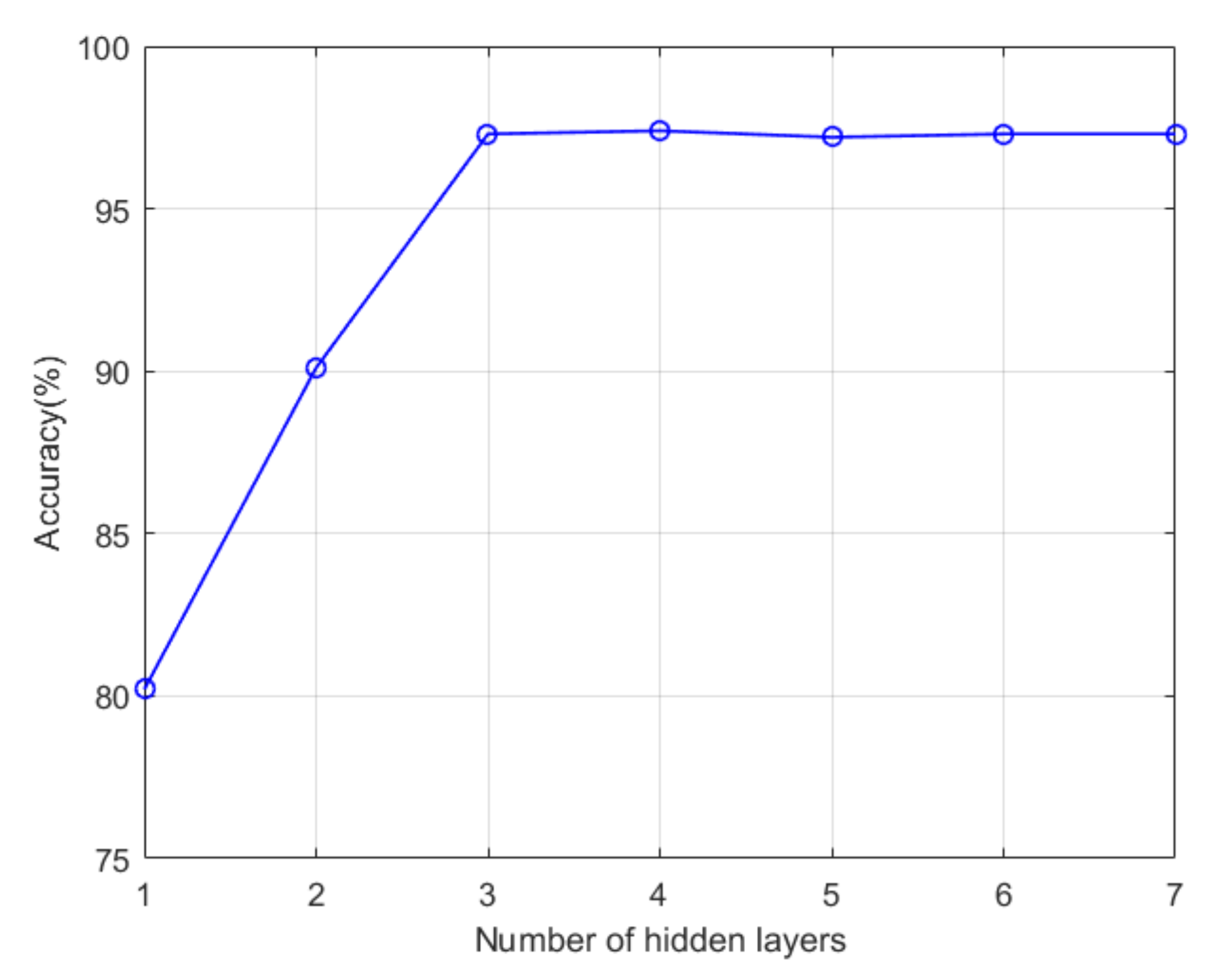
Like all other deep learning models, this paper uses a large number of experiments to select network structure parameters. Considering the dimensionality of the sample and the total number of participating samples, the range of the number of hidden layers is , and the number of hidden layer neurons is . Within the value range, 500 groups select randomly from all possible network structure configurations for experiments. The parameter configuration corresponding to the smallest error is selected as the optimal parameter setting. The network structure’s optimal parameters are: the number of hidden layers is 3, and the number of neurons corresponding to each layer is 256, 128, and 64.
After obtaining the optimal parameters of the model, the network structure parameters’ sensitivity will be analyzed below, that is, investigating a specific parameter, with all other fixed parameters, and the impact of parameter changes on the accuracy of the model will be examined.
Figure 5 is a graph of model accuracy as a function of the number of hidden layers. When using a hidden layer, the precision of the model is about 80%. The main reason for the lower accuracy is that there are too few weight parameters in the neural network. There is insufficient ability to represent the sample’s statistical feature information. When the number of hidden layers is 3, the accuracy of the current sample labeling model has reached the maximum. Continuously increasing the number of layers leads to over-fitting the model, which affects the model’s generalization ability, and the accuracy rate in the test set shows a downward trend.
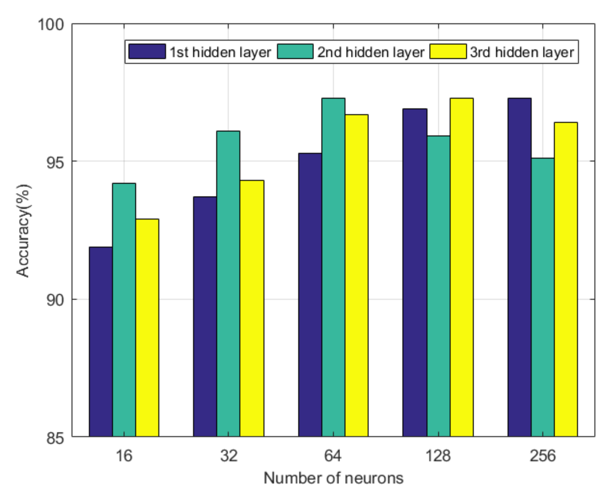
Finally, we fix the number of hidden layers and analyze the influence of the number of neurons on the performance of the model. Due to a large number of neuron combinations, it is not possible to display all of them. The neurons of each hidden layer are analyzed separately. We fix neurons in other hidden layers and examine the impact of model performance when the hidden layer changes.
Figure 6 shows the experimental results of the number of neurons on the model’s performance. When the number of neurons in two layers is fixed, the farther the number of neurons in the other layer is from the optimal value, the worse the model performance. It is further found that the number of neurons in each layer decreased from the first layer to the third hidden layer. For the first hidden layer, the accuracy rate increases with the number of neurons. This result is mainly due to the effect of the sparse encoder. Because the input data dimensions are small, to characterize the coupling relationship between the attributes of the input data better, the first hidden layer needs more neurons to participate in the representation. For the third hidden layer, the number of neurons is small, closely related to the congestion level’s classification into three categories. Since the output layer has only three neurons, it is obtained by applying the softmax function to the third layer’s hidden layer. If the number of neurons in the hidden layer is too large, softmax classification becomes difficult.
4.4. Performance Analysis
In this section, we first analyze the impact of sample collection strategy and initial sample size on model performance. We then compare it with mainstream methods to verify the effectiveness and superiority of the model.
4.4.1. Effect of Sample Label Strategy on Model Performance
This paper uses active learning to train the congestion recognition model based on a deep sparse autoencoder. During the model training process, each iteration needs to use a sample label strategy to select samples from the unlabeled sample set for labeling. The following experiments verify the impact of different labeling strategies on model performance. S3 was chosen as an experimental case. Each time, 300 samples were selected from the unlabeled sample set for labeling. Different sample label strategies are utilized for training the models and comparing their performance during the iteration process.
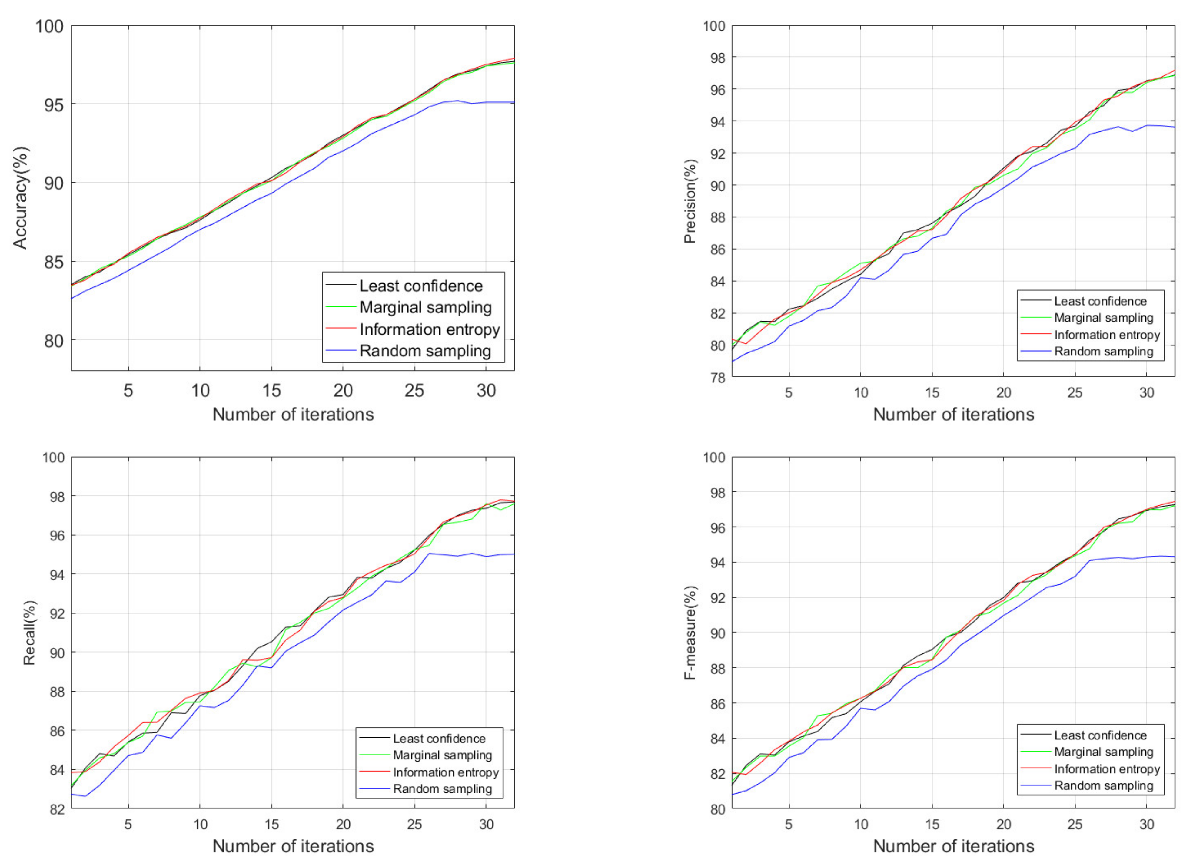
Figure 7 shows the experimental results of four label strategies, where the horizontal ordinate indicates the iteration number of the active learning process. This figure suggests that each of the four label strategies has an increasing trend with the increase of iterations. Random sampling has the worst performance. The performance of least confidence, marginal sampling, and information entropy is not much different. The main reason for this result is that the samples selected by minimum confidence, marginal sampling, and information entropy are more representative than random sampling. Thus, the labeled sample set has less data redundancy.
It is further found that when the number of iterations reached 26, the curve of the label strategy based on random sampling started to flatten, and the model performance reached its peak. In contrast, the other three label strategies slowed down but still showed an upward trend. The optimal value is reached when the number of iterations is 33. After 26 iterations, the unlabeled sample set itself has much redundancy by analyzing the remaining unlabeled samples. Because samples selected by the random sampling method are highly similar to the labeled sample set, it will not help improve the recognition rate even if one continues to increase the labeled training set. Consequently, the other three label strategies can still find samples that differ from the features of the labeled set from the remaining unlabeled samples. In general, the sample labeling strategies of minimum confidence, marginal sampling, and information entropy are better than random sampling. Information entropy is slightly better than minimum confidence and marginal sampling. Given this, in the following experiments, the information entropy is utilized to label samples.
4.4.2. Effect of the Number of Initial Labeled Samples on Model Performance
The method proposed in this paper is inherently iterative semi-supervised learning. Before the iteration, the hidden layer features of the deep learning model are constructed by initial training of the model, that is, the sparse autoencoding method is used to extract the features of labeled and unlabeled samples. Further, the initial labeled samples are utilized for training the parameters of the regression layer. The purpose of the active learning method is to train a model that meets the required performance using as few labeled samples as possible. The number of initial labeled samples on the performance of the model is analyzed experimentally to provide a basis for selecting the initial labeled samples.
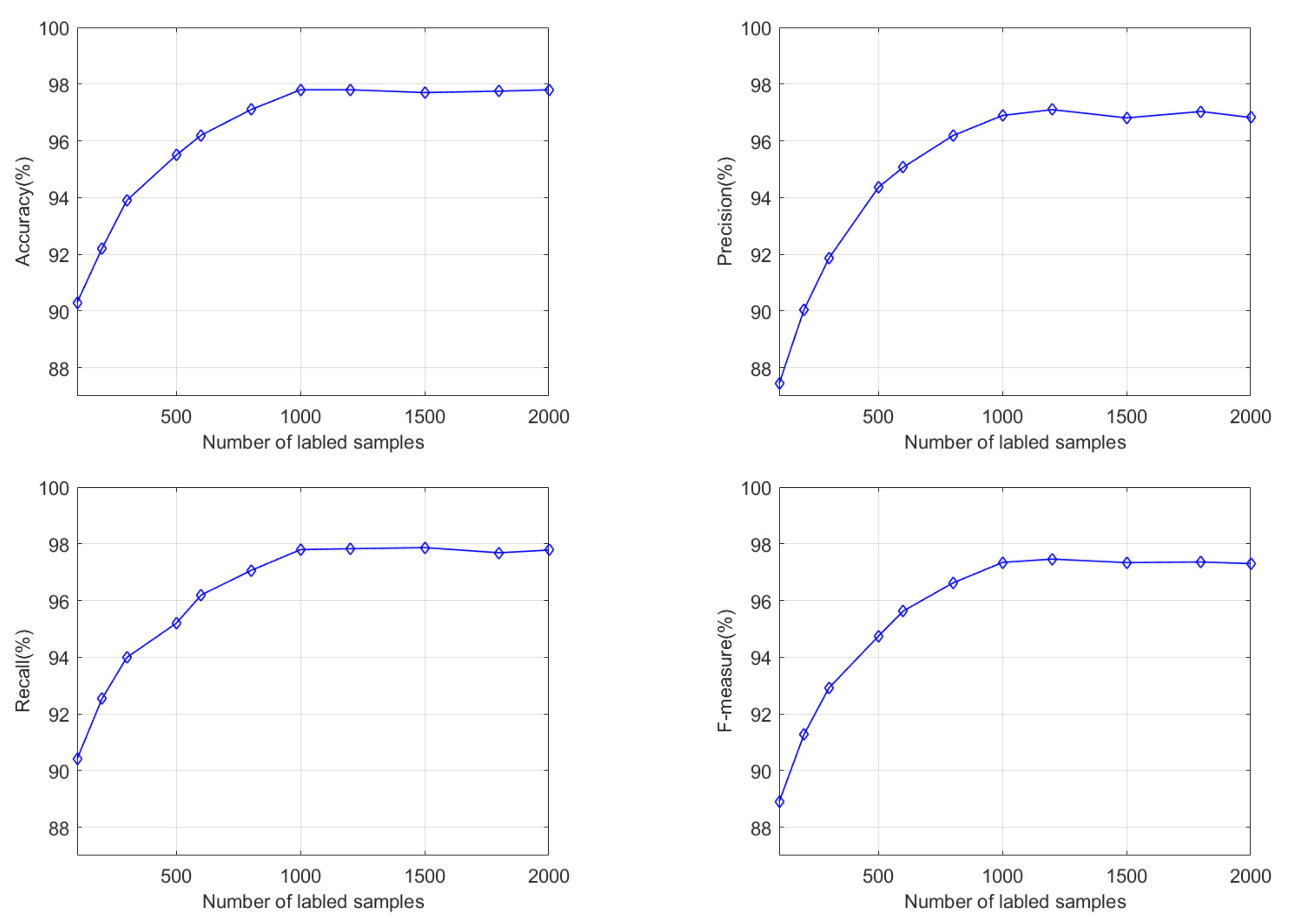
Figure 8 is the experimental result of the initial labeled sample number in the range of 100 to 2000. When the number of initial samples is 100, the accuracy, precision, recall, and F-measure values are 90.30%, 87.44%, 90.41%, and 88.90%, respectively. The performance of the model is relatively good. The main reason is that there are continually new labeled samples to modify the model during the active learning iteration process. Due to too few initial marking samples, the initial model’s performance is weak, which is far from the ideal requirement. As the number of initial samples increases, the performance of the initial model improves, and the final model also adjusts accordingly. When the initial sample size sets to 1000, the model performance reaches the optimal state. If the number of initial labeled samples increases, the performance improvement is minimal. By considering the relationship between model performance and the initial labeling sample, it is more appropriate to select 1000 labeled samples when training the model.
4.4.3. Comparative Analysis of Different Methods
To verify the superiority of our proposed method, the deep active learning method (referred to as DAL in this experiment) is compared with PCA-BPNN [
23] and GFSS-SVM [
24].
Table 2 and
Figure 9 show the experimental results. According to the results presented in
Table 2, as a whole, DAL maintained above 97% in the four indices. In contrast, although the accuracy, precision, recall, and measurement values of PCA-BPNN and GFSS-SVM are all over 90%, PCA-BPNN and GFSS-SVM are lower than DAL by about 4.5% and 2.5%, respectively. It is because PCA-BPNN belongs to shallow feed-forward neural networks with limited ability to characterize input features, resulting in lower model performance. Similarly, the essence of GFSS-SVM is to use the SVM method for classification. SVM only supports two classifications. Multi-classification must combine multiple support vector machines. For large sample classification problems, training is time-consuming, and performance is relatively poor.
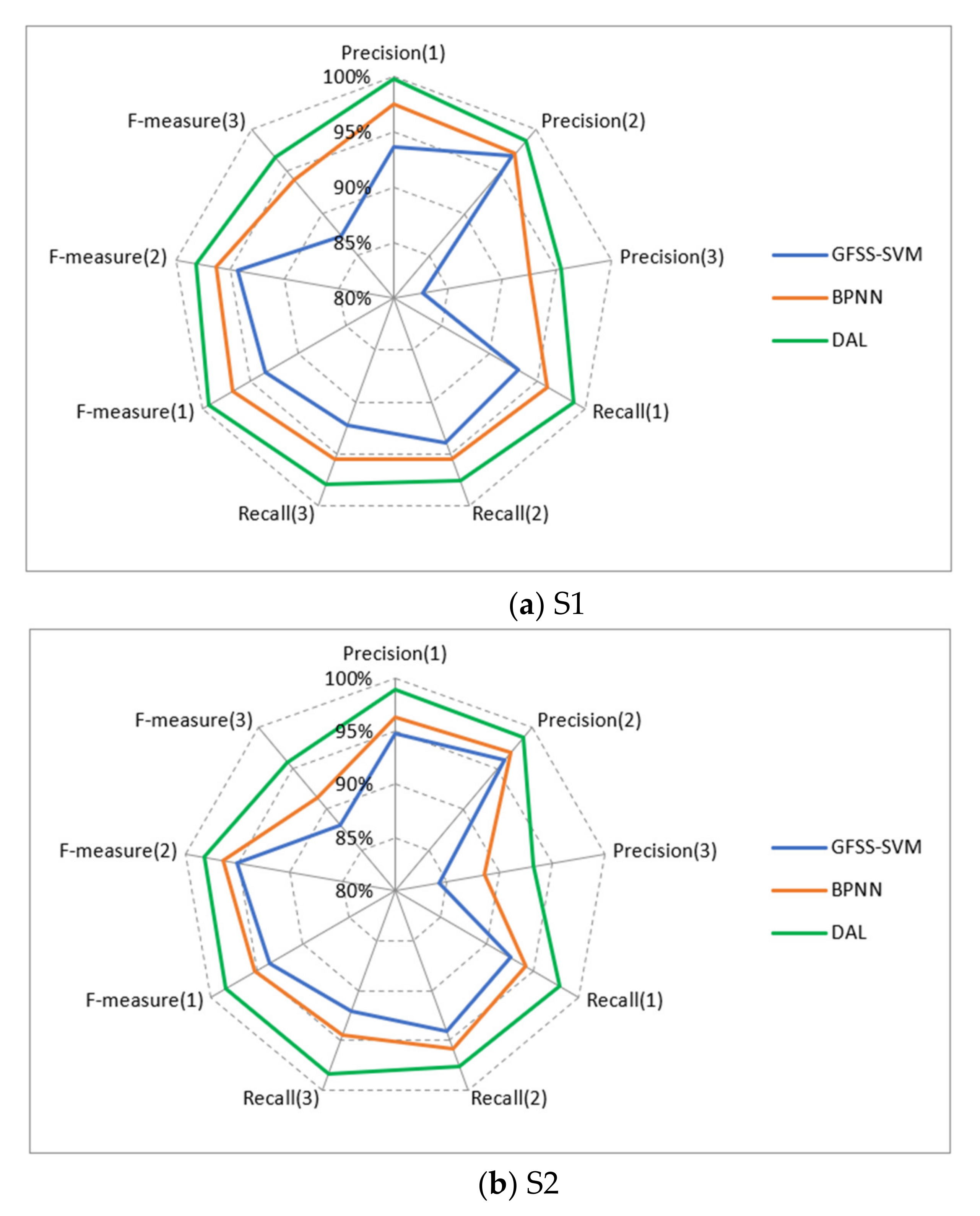
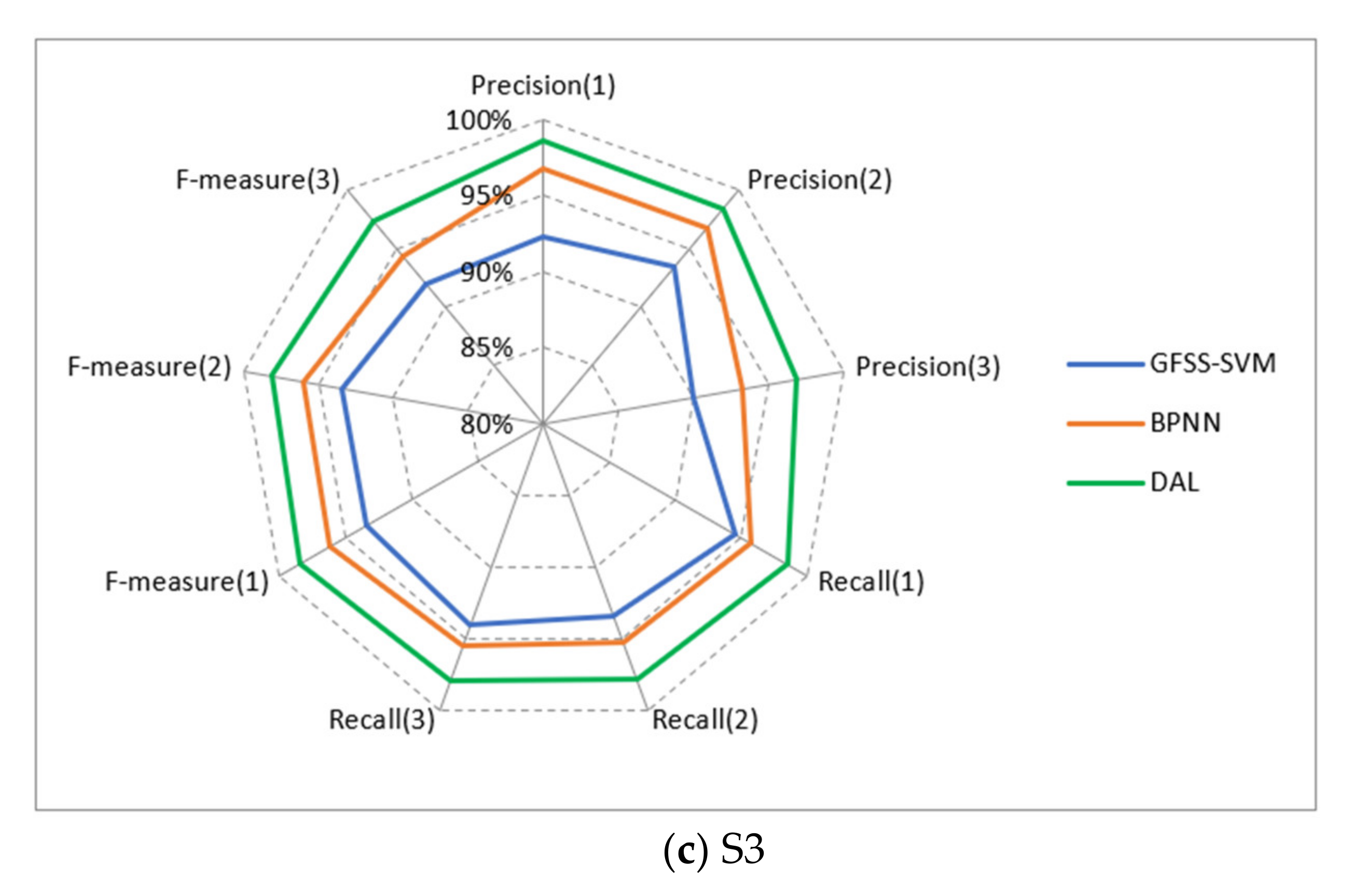
Figure 9 shows the recognition results of three representative sectors using different methods. For S2, the accuracy of GFSS-SVM and BPNN is less than 90%, and the accuracy of DAL is about 94%. The main reason for this result is the class imbalance of the sample set. Compared with congestion categories 1 and 2, congestion category 3 is heavily congested and belongs to a few extreme cases in daily operation. The proportion of samples available for model learning is less than 10%, so the trained model has a relatively low accuracy for the congestion category of 3. S3 belongs to a class of busy sectors, and the congestion is moderately severe. The proportion of samples with category three participating in training exceeds 25%. Therefore, in S3, the effect on the congestion category of 3 is better than that of S1 and S2.
In general, DAL is superior to the mainstream GFSS-SVM and BPNN in both the overall performance and each type of congestion level. Additionally, for sectors with different busy levels, DAL can still achieve a relatively high recognition rate due to the imbalance of samples, proving that our approach has a good generalization ability.
5. Conclusions
In order to improve the generalization ability of the model and overcome the high cost of sample labeling, this paper proposes an ATCS congestion recognition method based on deep active learning, which obtains a high recognition rate with the least labeled samples. This method has strategic and tactical significance. It can not only provide a basis for the merging and addition of sectors, but also identify the congestion of sectors in real-time, and provide a more intuitive reference for controllers to provide control services. The proposed method consists of two modules, the congestion recognition model based on deep sparse autoencoding and the sample labeling strategy, which adopts an iterative semi-supervised manner.
The network structure of the congestion recognition model based on deep sparse autoencoding consists of a feature input layer, multiple hidden layers, and a regression output layer. Before iterative training of the model, we employed a sparse autoencoder to perform feature learning on all labeled and unlabeled samples, constructed a hidden layer in a stacked manner, and used labeled samples to determine the regression layer. Because the model uses only a few labeled samples in the initial training stage, the trained model has relatively poor performance. It needs to select a certain number of samples from the unlabeled sample set for labeling. To this end, we introduced three sample labeling strategies: minimum confidence, marginal sampling, and information entropy. Samples with substantial feature differences from the labeled sample set are chosen from the unlabeled sample set. This can reduce the data redundancy in the labeled sample set, thereby achieving the desired model performance with smaller label samples.
Finally, this paper used three representative sectors with different airspace structures and flight flows. The experimental results demonstrated that the number of initial labeled samples affects the performance of the model. For the three types of congestion levels, it is appropriate to choose 1000 initial label samples. At the same time, we verified the three sample label strategies. The results showed that the three sampling strategies are almost equivalent and better than the commonly used random sampling method. The information entropy is slightly better than the minimum confidence and marginal sampling. To verify the superiority of our proposed method, we compared it with two mainstream methods. The experimental results suggested that our approach is superior to the mainstream approaches in accuracy, precision, recall rate, and F-measure.


