Maneuvering Spacecraft Orbit Determination Using Polynomial Representation

Abstract

This paper proposed a polynomial representation-based method for orbit determination (OD) of spacecraft with the unknown maneuver. Different from the conventional maneuvering OD approaches that rely on specific orbit dynamic equation, the proposed method needs no priori information of the unknown maneuvering model. The polynomials are used to represent the unknown maneuver. A transformation is made for the polynomials to improve the convergence and robustness. The Extended Kalman Filter (EKF) is used to process incoming observation data by compensating the unknown maneuver using the polynomials. The proposed method is successfully applicated into the OD problem of spacecraft with trigonometric maneuver. Numerical simulations show that the eighth-order polynomials are accurate enough to represent a trigonometric maneuver. Moreover, Monte Carlo simulations show that the position errors are smaller than 1 km, and the maneuver estimated errors are no more than 0.1 mm/s² using the eighth-order polynomials. The proposed method is accurate and efficient, and has potential applications for tracking maneuvering space target.

1. Introduction

Orbit determination (OD) is an important task in space missions, as knowing the state of the spacecraft is the basis of the subsequent operations such as the guidance and control [1,2,3]. One of the hard issues of OD is tracking a spacecraft with unknown maneuvering accelerations [4,5]. These unknown maneuvers can be caused by an uncooperative orbit control [6], structural deployment [7], collisions [8] and space environment changes [9,10]. The unknown maneuver incurs severe uncertainty into the state model [9]. Without compensating the uncertainty, the state model is inaccurate, and thus the OD performance is degraded [11].

The state-of-the-art techniques for maneuvering spacecraft OD can be classified into the following three catalogues: OD reinitiating, maneuver reconstruction and filter-based methods. The first kind of methods are to reinitiate an OD process once a maneuver is detected [6,12]. These methods disregard the pre-maneuver solutions and measurements, and determine a new orbit for the target [13]. The OD reinitiating methods rely on the detection of the maneuver and usually have poor performance in accuracy. The maneuver reconstruction methods estimate both the orbit and the maneuver using the measurement pre and post the maneuver [14,15]. The main procedures of the maneuver reconstruction are establishing the equations and then solving them with all the measurements included. They can provide more accurate solutions while involve much more complexity and computational burden, and are impossible for real-time applications [16,17].

The filter-based methods establish models to fit the unknown maneuver [18,19,20]. These models are involved in the filtering process to compensate the uncertainty caused by the unknown maneuver [21]. The filter-based methods also estimate both the orbit and the maneuver. Compared with the maneuver reconstruction methods, the filter-based methods have one distinguished feature. The maneuver reconstruction method is usually a post-processing. The filter-based methods fit the post-maneuver information into the existing pre-maneuver orbit. After the compensated model is established, the filter algorithm can be used to solve the maneuvering OD problem step by step, which is a real-time tracking process. A number of technologies have been developed for the filter-based methods. Zhai et al. developed a variable structure estimator (VSE) based approach for tracking uncooperative spacecraft with unknown maneuvers [22,23]. The VSE is used to estimate the unknown maneuver and is fed to an extended Kalman filter (EKF) as a compensation. Ko and Scheeres proposed a real time tracking method based on the Thrust-Fourier-coefficient (TFC) event representation [9]. The TFC event representation is employed to explicitly estimate the unknown control. Maybeck and Hentz investigated a moving-bank multiple model adaptive estimated filter for tracking maneuvering target [24]. The multiple model methods use a bank of Kalman filters with different maneuvering models [25]. Each maneuvering model corresponds to a particular maneuvering dynamic. Moreover, motivated by the fast development of the artificial intelligence, some deep learning techniques have been used for solving problems related to the maneuvering object OD, such as the maneuver detection [26], maneuver classification [27] and maneuvering spacecraft orbit prediction [28,29].

Compared with the maneuver reconstruction methods, the filter-based methods have much lower computational burden [9,30,31]. Moreover, the filter-based method does not rely on maneuver detection, and has better accuracy than the OD reinitiating approaches. The only defect of the current filter-based methods is that they are based on particular assumptions on the maneuvering model. For example, to use the TFC event representation, the unknown maneuver should be periodic [9]. When the assumptions do not match the real maneuver, the performance of these methods will degrade [32]. Thus, a motivation is generated that, it is necessary to investigate a general mathematical representation that can approximate any form of the unknown maneuver. In this way, the filter-based methods can be released from the specific assumptions.

The proposed polynomial representation-based method in this paper falls into the filter-based methods. Different from other filter-based methods, it does not need any assumptions or priori information about the unknown maneuver. The polynomials with respect to time are firstly established to fit the unknown maneuver. The polynomial representation is expected to have the ability to cope with any unknown maneuvers. A transformation is made for these polynomials to eliminate the sensitivity of the high-order terms of time. In this way, the numerical singularity related to the high-order polynomial terms is avoided, and the convergence and robustness of the OD system are improved. The polynomial representation is expected to accurately fit any kinds of the maneuver, and has a fast convergence. The EKF process is then fused with the polynomial representation to estimate the maneuvering orbit. The performance of the proposed methods is validated across different maneuvering cases.

The rest of this paper is arranged as follows. The state and the measurement models are given in Section 2. Section 3.1 firstly details the polynomial representation for fitting unknown maneuver. The EKF process combined with the polynomial representation is introduced in the subsequent subsection. Observability analysis is implemented in Section 4. Numerical simulations are performed in Section 5, and conclusions are discussed in Section 6.

2. Problem Formulation

2.1. State Model

Consider a space-based maneuvering spacecraft tracking problem. In this scenario, two spacecraft, a target and an observer, are involved. The inter-spacecraft relative range/velocity measurement is used based on the radio. The ratio measurement is chosen to validate the performance of the proposed method in an owe-observation condition.

An Earth-centered dynamic with unknown maneuver is shown as follows: [9,33]:

$$\left\{\begin{array}{c}{\dot{\mathit{r}}}_T={\mathit{v}}_T\hfill \\ {\dot{\mathit{v}}}_T=\underset{\mathit{f}\left({\mathit{r}}_T\right)}{\underbrace{-\frac{{\mu }_e}{{∥{\mathit{r}}_T∥}^3}{\mathit{r}}_T+{\mu }_s\left(\frac{{\mathit{r}}_s-{\mathit{r}}_T}{{∥{\mathit{r}}_s-{\mathit{r}}_T∥}^3}-\frac{{\mathit{r}}_s}{{∥{\mathit{r}}_s∥}^3}\right)+{\mu }_m\left(\frac{{\mathit{r}}_m-{\mathit{r}}_T}{{∥{\mathit{r}}_m-{\mathit{r}}_T∥}^3}-\frac{{\mathit{r}}_m}{{∥{\mathit{r}}_m∥}^3}\right)+{\mathit{a}}_{J_2}\left({\mathit{r}}_T\right)}}+{\mathit{a}}_c\hfill \end{array}\right.$$

(1)

where ${\mathit{x}}_T=\left[{\mathit{r}}_T;{\mathit{v}}_T\right]={\left[x_T,y_T,z_T,{\dot{x}}_T,{\dot{y}}_T,{\dot{z}}_T\right]}^T$ denotes the state of the maneuvering target; ${\mu }_e$, ${\mu }_s$ and ${\mu }_m$ are the gravitational constant of the Earth, the Sun and the Moon, respectively; ${\mathit{r}}_s$ and ${\mathit{r}}_m$ label positions of the Sun and Moon relative to the Earth; ${\mathit{a}}_{J_2}(·)$ is the perturbation acceleration of J₂; $\mathit{f}(·)$ contains all the modeled parts of the dynamics and ${\mathit{a}}_c$ is the unknown maneuvering acceleration.

Assume that the dynamics of the observer spacecraft is known and is given as:

$$\left\{\begin{array}{c}{\dot{\mathit{r}}}_O={\mathit{v}}_O\hfill \\ {\dot{\mathit{v}}}_O=\mathit{f}\left({\mathit{r}}_O\right)\hfill \end{array}\right.$$

(2)

where ${\mathit{x}}_O=\left[{\mathit{r}}_O;{\mathit{v}}_O\right]={\left[x_O,y_O,z_O,{\dot{x}}_O,{\dot{y}}_O,{\dot{z}}_O\right]}^T$ is the state of the observer.

2.2. Measurement Model

The inter-spacecraft range/velocity measurement is written as [34]:

$$\mathit{z}=\mathit{h}\left({\mathit{x}}_T\right)+\mathit{\epsilon }=\left[\begin{array}{c}\rho +{\epsilon }_{\rho }\\ \dot{\rho }+{\epsilon }_{\rho }\end{array}\right]=\left[\begin{array}{c}∥{\mathit{r}}_O-{\mathit{r}}_T∥+{\epsilon }_{\rho }\\ \frac{{\left({\mathit{v}}_O-{\mathit{v}}_T\right)}^T\left({\mathit{r}}_O-{\mathit{r}}_T\right)}{∥{\mathit{r}}_O-{\mathit{r}}_T∥}+{\epsilon }_{\rho }\end{array}\right]$$

(3)

where $\mathit{h}\left({\mathit{x}}_T\right)$ denotes the measurement function; $\rho$ and $\dot{\rho }$, respectively, label the inter-spacecraft range and the velocity; $\mathit{\epsilon }={\left[{\epsilon }_{\rho },{\mathit{\epsilon }}_{\dot{\rho }}\right]}^T$ is the Gaussian-distributed measurement noise.

The goal of the maneuvering spacecraft OD is to estimate the state of the target ${\mathit{x}}_T$. Combine Equation (3) with Equation (1), and the OD system is given as:

$$\left\{\begin{array}{c}{\dot{\mathit{x}}}_T=\left[{\mathit{v}}_T;\mathit{f}\left({\mathit{x}}_T\right)+{\mathit{a}}_c\right]\hfill \\ \mathit{z}=\mathit{h}\left({\mathit{x}}_T\right)+\mathit{\epsilon }\hfill \end{array}\right.$$

(4)

3. Orbit Determination Using Polynomial Representation

3.1. Polynomial Representation for Unknown Maneuver

Let $a_x\left(t\right)$, $a_y\left(t\right)$ and $a_z\left(t\right)$ denote the components of the unknown maneuvering acceleration along the x-axis, y-axis and z-axis, respectively. The unknown maneuvering acceleration can be approximated by a polynomial. The corresponding polynomial representation is proposed as follows:

$$\left\{\begin{array}{c}{a}_x\left(t\right)=\sum _{i=0}^{\infty }{p}_{x,i}{\left(\frac{t}{T}\right)}^i=p_{x,0}+p_{x,1}\frac{t}{T}+p_{x,2}{\left(\frac{t}{T}\right)}^2+\cdots +p_{x,i}{\left(\frac{t}{T}\right)}^i+\cdots \hfill \\ a_y\left(t\right)=\sum _{i=0}^{\infty }{p}_{y,i}{\left(\frac{t}{T}\right)}^i=p_{y,0}+p_{y,1}\frac{t}{T}+p_{y,2}{\left(\frac{t}{T}\right)}^2+\cdots +p_{y,i}{\left(\frac{t}{T}\right)}^i+\cdots \hfill \\ a_z\left(t\right)=\sum _{i=0}^{\infty }{p}_{z,i}{\left(\frac{t}{T}\right)}^i=p_{z,0}+p_{z,1}\frac{t}{T}+p_{z,2}{\left(\frac{t}{T}\right)}^2+\cdots +p_{z,i}{\left(\frac{t}{T}\right)}^i+\cdots \hfill \end{array}\right.$$

(5)

where $p_{x,i}$, $p_{y,i}$ and $p_{z,i}$ are the coefficients of the i-th order terms; T is a user-defined normalized period. In Equation (5), the time t is normalized by T to reduce the sensitivity of polynomials to the high-order coefficients. Obviously, higher-order polynomials provide more precise approximations, and the convergence of the estimation algorithm will be better. However, high-order polynomials contain many coefficients, which make the computational overhead unacceptable. Thus, to balance the accuracy, convergence and the time cost of the algorithm, it is necessary compare the performance of the polynomials with different orders. The comparisons and the discussion are shown in Section 5.1.

There are two possible ways to fuse the polynomial representation into the OD system. The first way is to directly use the Equation (5) and the OD system estimates both the orbit and the coefficients $p_{x,i}$, $p_{y,i}$ and $p_{z,i}$. In this case, ${\dot{p}}_{x,i}={\dot{p}}_{y,i}={\dot{p}}_{z,i}=0$. However, to the authors’ best knowledge, the OD system will be hard to converge if Equation (5) is directly employed to compensate the unknown maneuver. It is because the coefficients $p_{x,i}$, $p_{y,i}$ and $p_{z,i}$ in Equation (5) are equally important to the OD system and therefore an accurate OD can be obtained only when all these coefficients converge. Moreover, for cases where t is very large, the high-order term of t is large. Thus, the coefficients of the high-order terms should be very small, which put forward the requirement of highly precise numerical calculation. To improve the convergence and robustness, the second way is employed, and a transformation is made, which is described as below. First, define the auxiliary variables as follows:

$$\begin{array}{c}{a}_{\alpha ,0}=\sum _{i=0}^{\infty }{p}_{\alpha ,i}{\left(\frac{t}{T}\right)}^i=p_{\alpha ,0}+p_{\alpha ,1}\frac{t}{T}+p_{\alpha ,2}{\left(\frac{t}{T}\right)}^2+\cdots +p_{\alpha ,i}{\left(\frac{t}{T}\right)}^i+\cdots \hfill \\ a_{\alpha ,1}={\left[\sum _{i=0}^{\infty }{p}_{\alpha ,i}{\left(\frac{t}{T}\right)}^i\right]}^{\prime }=\frac{1}{T}\sum _{i=1}^{\infty }i{p}_{\alpha ,i}{\left(\frac{t}{T}\right)}^{i-1}=p_{\alpha ,1}\frac{1}{T}+2p_{\alpha ,2}\frac{t}{T^2}+\cdots +\frac{1}{T}i{p}_{\alpha ,i}{\left(\frac{t}{T}\right)}^{i-1}+\cdots \hfill \\ a_{\alpha ,2}={\left[\sum _{i=0}^{\infty }{p}_{\alpha ,i}{\left(\frac{t}{T}\right)}^i\right]}^{″}=\frac{1}{T}\sum _{i=2}^{\infty }i(i-1)p_{\alpha ,i}{\left(\frac{t}{T}\right)}^{i-2}=2p_{\alpha ,2}\frac{1}{T}+6p_{\alpha ,3}\frac{t}{T^2}\cdots +\frac{1}{T}i(i-1)p_{\alpha ,i}{\left(\frac{t}{T}\right)}^{i-2}+\cdots \hfill \\ \cdots \hfill \\ a_{\alpha ,k}={\left[\sum _{i=0}^{\infty }{p}_{\alpha ,i}{\left(\frac{t}{T}\right)}^i\right]}^{\left(k\right)}=\frac{1}{T}\sum _{i=k}^{\infty }\left(\prod _{m=i-k+1}^{i}m\right)p_{\alpha ,i}{\left(\frac{t}{T}\right)}^{i-k}=\frac{1}{T}\left(\prod _{m=1}^{k}m\right)p_{\alpha ,k}+\left(\prod _{m=2}^{k+1}m\right)p_{\alpha ,k+1}\frac{t}{T^2}+\cdots \hfill \\ \cdots \hfill \end{array}$$

(6)

where $\alpha \in \{x,y,z\}$ denotes the subscript.

Let ${\mathit{a}}_k={\left[a_{x,k},a_{y,k},a_{z,k}\right]}^T$, and Equation (6) can be simplified as:

$$\begin{array}{c}{\mathit{a}}_c={\mathit{a}}_0\hfill \\ {\dot{\mathit{a}}}_0={\mathit{a}}_1\hfill \\ {\dot{\mathit{a}}}_1={\mathit{a}}_2\hfill \\ \cdots \hfill \\ {\dot{\mathit{a}}}_k={\mathit{a}}_{k+1}\hfill \\ \cdots \hfill \end{array}$$

(7)

In this way, the states representing the unknown maneuver are replaced by the coefficients ${\mathit{a}}_{k+1}$, ${\mathit{a}}_k$, ${\mathit{a}}_1$ and ${\mathit{a}}_0$. Two advantages can benefit from the transformation. Firstly, the coefficients ${\mathit{a}}_{k+1}$, ${\mathit{a}}_k$, ${\mathit{a}}_1$ and ${\mathit{a}}_0$ can gradually converge, which enhances the convergence of the OD system. Secondly, the influence of the time t is eliminated from the polynomial representation, and thus the numerical singular is avoided.

3.2. Extended Kalman Filter with Polynomial Representation

Use the polynomials up to k-th order and the state to be estimated is written as:

$$\mathit{X}=\left[{\mathit{r}}_T;{\mathit{v}}_T;{\mathit{a}}_0;{\mathit{a}}_1;\cdots ;{\mathit{a}}_k\right]$$

(8)

The state model of the OD system is then given by:

$$\dot{\mathit{X}}=\left[\begin{array}{c}{\dot{\mathit{r}}}_T\hfill \\ {\dot{\mathit{v}}}_T\hfill \\ {\dot{\mathit{a}}}_0\hfill \\ {\dot{\mathit{a}}}_1\hfill \\ {\dot{\mathit{a}}}_2\hfill \\ \cdots \hfill \\ {\dot{\mathit{a}}}_k\hfill \end{array}\right]=\left[\begin{array}{c}{\mathit{v}}_T\hfill \\ \mathit{f}\left({\dot{\mathit{r}}}_T\right)+{\mathit{a}}_0\hfill \\ {\mathit{a}}_1\hfill \\ {\mathit{a}}_2\hfill \\ {\mathit{a}}_3\hfill \\ \cdots \hfill \\ {\mathbf{0}}_{3\times 1}\hfill \end{array}\right]$$

(9)

and the measurement model is given as:

$$\mathit{z}=\mathit{h}\left(\mathit{X}\right)+\mathit{\epsilon }=\mathit{h}\left({\mathit{x}}_T\right)+\mathit{\epsilon }=\left[\begin{array}{c}\rho +{\mathit{\epsilon }}_{\rho }\\ \dot{\rho }+{\epsilon }_{\dot{\rho }}\end{array}\right]$$

(10)

The state transition matrix (STM) of the state model (9) is partitioned as:

$$\mathbf{\Phi }\left(t_0,t\right)=\frac{\partial \mathit{X}\left(t\right)}{\partial \mathit{X}\left(t_0\right)}=\left[\begin{array}{cc}{\mathbf{\Phi }}_{xx}\left(t_0,t\right)\hfill & {\mathbf{\Phi }}_{xa}\left(t_0,t\right)\hfill \\ {\mathbf{\Phi }}_{ax}\left(t_0,t\right)\hfill & {\mathbf{\Phi }}_{aa}\left(t_0,t\right)\hfill \end{array}\right]$$

(11)

The differential equation of the STM can be expressed as:

$$\dot{\mathbf{\Phi }}\left(t_0,t\right)=\mathbf{A}\left(t\right)\mathbf{\Phi }\left(t_0,t\right)=\left[\begin{array}{cc}{\mathbf{A}}_{xx}\left(t\right)\hfill & {\mathbf{A}}_{xa}\left(t\right)\hfill \\ {\mathbf{A}}_{ax}\left(t\right)\hfill & {\mathbf{A}}_{aa}\left(t\right)\hfill \end{array}\right]\left[\begin{array}{cc}{\mathbf{\Phi }}_{xx}\left(t_0,t\right)\hfill & {\mathbf{\Phi }}_{xa}\left(t_0,t\right)\hfill \\ {\mathbf{\Phi }}_{ax}\left(t_0,t\right)\hfill & {\mathbf{\Phi }}_{aa}\left(t_0,t\right)\hfill \end{array}\right]$$

(12)

where $\mathbf{A}\left(t\right)$ is the Jacobian matrix of the state model:

$${\mathbf{A}}_{xx}\left(t\right)=\frac{\partial \mathit{f}\left({\mathit{x}}_T\left(t\right)\right)}{\partial {\mathit{x}}_T\left(t\right)}\in {\mathbb{R}}^{6\times 6}$$

(13)

$${\mathbf{A}}_{xa}\left(t\right)=\left[\begin{array}{cc}{\mathbf{0}}_{3\times 3}& {\mathbf{0}}_{3\times \left(3k\right)}\\ {\mathit{I}}_3& {\mathbf{0}}_{3\times \left(3k\right)}\end{array}\right]\in {\mathbb{R}}^{6\times (3k+3)}$$

(14)

$${\mathbf{A}}_{ax}\left(t\right)={\mathbf{0}}_{(3k+3)\times 6}\in {\mathbb{R}}^{(3k+3)\times 6}$$

(15)

$${\mathbf{A}}_{aa}\left(t\right)=\left[\begin{array}{ccccc}{\mathbf{0}}_{3\times 3}& {\mathit{I}}_3& {\mathbf{0}}_{3\times 3}& \cdots & {\mathbf{0}}_{3\times 3}\\ {\mathbf{0}}_{3\times 3}& {\mathbf{0}}_{3\times 3}& {\mathit{I}}_3& \cdots & {\mathbf{0}}_{3\times 3}\\ ⋮& ⋮& ⋮& \ddots & ⋮\\ {\mathbf{0}}_{3\times 3}& {\mathbf{0}}_{3\times 3}& {\mathbf{0}}_{3\times 3}& \cdots & {\mathit{I}}_3\\ {\mathbf{0}}_{3\times 3}& {\mathbf{0}}_{3\times 3}& {\mathbf{0}}_{3\times 3}& \cdots & {\mathbf{0}}_{3\times 3}\end{array}\right]\in {\mathbb{R}}^{(3k+3)\times (3k+3)}$$

(16)

According to Equations (8)–(16), the process of the EKF is formulated as follows.

3.2.1. Time Update

• Given the estimated state ${\widehat{\mathit{X}}}_{i-1}$ and covariance matrix ${\mathit{P}}_{i-1}$ at $t_{i-1}$.
• Calculate the predicted states ${\widehat{\mathit{X}}}_{i\mid i-1}$.

  $${\widehat{\mathit{X}}}_{i\mid i-1}=\mathit{F}\left({\widehat{\mathit{X}}}_{i-1}\right)$$

  (17)

  where $\mathit{F}(·)$ is the discrete form of the state model in Equation (9).
• Calculate the predicted covariance matrix ${\mathit{P}}_{i\mid i-1}$.

  $${\mathit{P}}_{i\mid i-1}={\mathbf{\Phi }}_i{\mathit{P}}_{i-1}{\mathbf{\Phi }}_i^T$$

  (18)

3.2.2. Measurement Update

• Calculate the predicted measurement ${\widehat{\mathit{z}}}_{i\mid i-1}$.

  $${\widehat{\mathit{z}}}_{i\mid i-1}=\mathit{h}\left({\widehat{\mathit{X}}}_{i\mid i-1}\right)$$

  (19)
• Calculate the predicted associated covariance ${\mathit{P}}_{{\mathit{x}}_z,i\mid i-1}$, ${\mathit{P}}_{zz,i\mid i-1}$.

  $$\begin{array}{c}{\mathit{P}}_{{\mathit{x}}_z,i\mid i-1}={\mathit{P}}_{i\mid i-1}{\mathit{H}}_i^T\hfill \\ {\mathit{P}}_{zz,i\mid i-1}={\mathit{H}}_i{\mathit{P}}_{i-1}{\mathit{H}}_i^T+{\mathit{R}}_i\hfill \end{array}$$

  (20)

  where ${\mathit{R}}_i$ is the covariance matrix of the measurement noise, ${\mathit{H}}_i$ is the Jacobian matrix of the measurement model:

  $${\mathit{H}}_i={\left.\frac{\partial \mathit{h}\left(\mathit{X}\right)}{\partial \mathit{X}}\right|}_{\mathit{X}={\widehat{\mathit{X}}}_{ii-1}}$$

  (21)
• On the receipt of the measurement ${\mathit{z}}_i$, calculate the estimated state ${\widehat{\mathit{X}}}_i$ and covariance matrix ${\mathit{P}}_i$ at $t_i$.

  $$\begin{array}{c}{\mathit{K}}_i={\mathit{P}}_{xz,i\mid i-1}{\mathit{P}}_{zz,i\mid i-1}^{-1}\hfill \\ {\widehat{\mathit{X}}}_i={\widehat{\mathit{X}}}_{i\mid i-1}+{\mathit{K}}_i\left({\mathit{z}}_i-{\widehat{\mathit{z}}}_{i\mid i-1}\right)\hfill \\ {\mathit{P}}_i={\mathit{P}}_{i\mid i-1}-{\mathit{K}}_i{\mathit{P}}_{zz,i\mid i-1}{\mathit{K}}_i^T\hfill \end{array}$$

  (22)

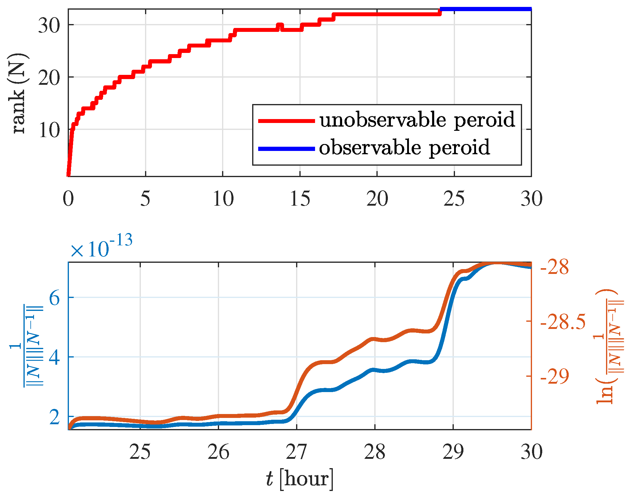
4. Observability Analysis

4.1. Observability Matrix

The OD using relative range/velocity measurements is inherently an owe-observation system. Moreover, the polynomial representations incur additional elements that are to be estimated. Thus, it is necessary to perform observability analysis to investigate whether the OD system is observable.

The observability matrix (OM) is used to measure the feasibility of an OD system [35,36,37]. Note that the OM is a way that evaluates the local observability, which is valid upon linearization of the system. A theoretical analysis can be conducted based on the OM to show the observable states or state combinations. The observations can be related to the states with a partial differential matrix ${\mathit{H}}_i$ at a future time t, as shown in Equation (21).

The matrix ${\mathit{H}}_i$ is mapped to the initial epoch $t_0$ through the STM as [35]:

$${\tilde{\mathit{H}}}_i={\mathit{H}}_i\mathbf{\Phi }\left(t_i,t_0\right)$$

(23)

By propagating from time epoch $t_0$ to $t_{i-1}$, measurements are collected sequentially, and each of ${\tilde{\mathit{H}}}_k(i=1,2,\cdots ,i-1)$ is derived according to Equation (23). Then, the OM $\mathit{N}$ is given by [35]:

$$\mathit{N}=\left[\begin{array}{c}{\tilde{\mathit{H}}}_0\\ {\tilde{\mathit{H}}}_1\\ ⋮\\ {\tilde{\mathit{H}}}_{i-2}\\ {\tilde{\mathit{H}}}_{i-1}\end{array}\right]$$

(24)

If the OM has a full rank, i.e., the columns of matrix $\mathit{N}$ are linearly independent with each other, the whole system is observable and all states can be estimated by a navigation filter. Furthermore, the invertibility of the OM, which is characterized by its singular values, is related to the degree of the observability of an OD system. In this paper, the condition number (CN) of OM is employed to numerically evaluate the degree of the observability. Denoting the largest and smallest singular values of the OM as ${\sigma }_{max}\left(\mathit{N}\right)$ and ${\sigma }_{min}\left(\mathit{N}\right)$, the CN is equal to the ratio ${\sigma }_{max}\left(N\right)/{\sigma }_{min}\left(N\right)$ (note that the CN could also be computed by $cond\left(\mathit{N}\right)=\parallel \mathit{N}\parallel ·\parallel {\mathit{N}}^{-1}\parallel$), which is interpreted as a relative index of observability of the best observable state relative to the worst observable state. Smaller CN usually implies better observability.

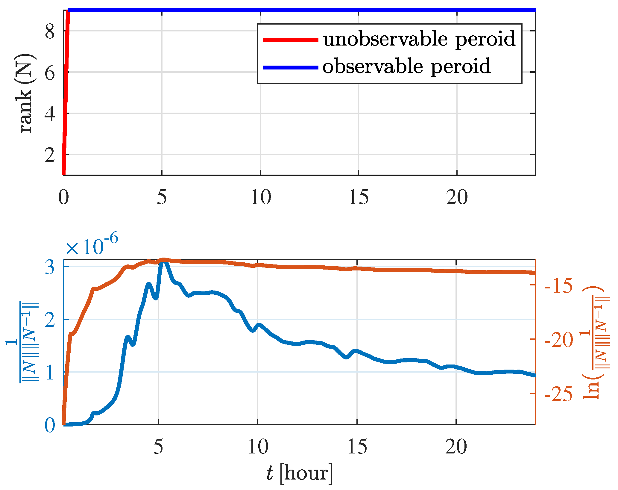
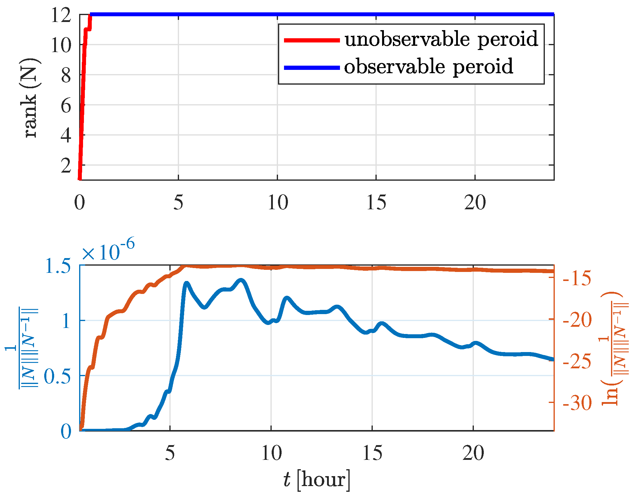
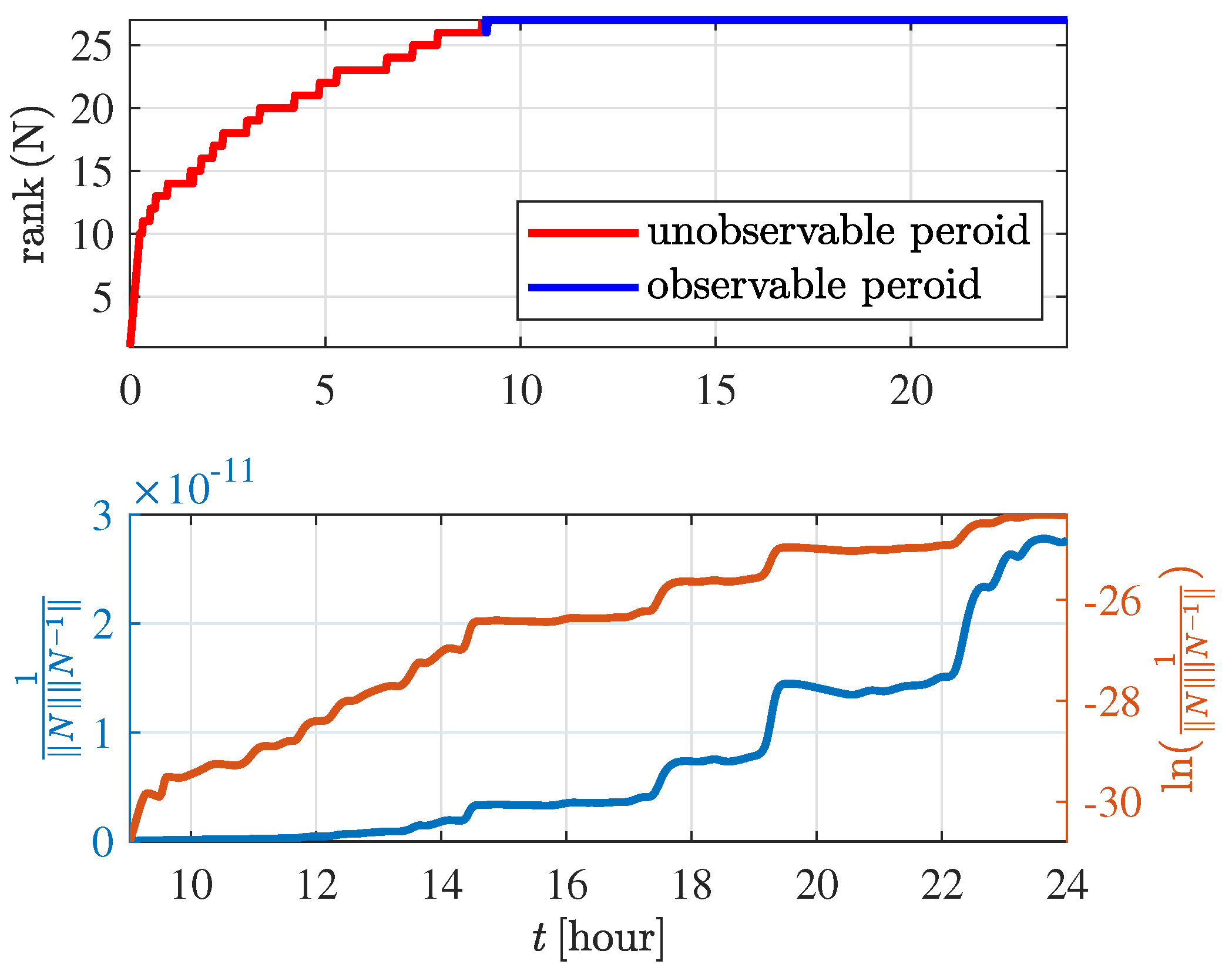
4.2. Observability Analysis Results

The nominal orbit elements of the target and observer are listed in

Table 1. Nominal orbit elements of the target and the observer.

	a/km	e	i/deg	$\mathbf{\Omega }$/deg	$\mathit{\omega }$/deg	n/deg
Target	8871.14	0.05	45	94.8	199.0	305.87
Observer	6871.14	0.01	45.5	29.93	132.9	252.26

, where a, e, n, i, $\omega$ and $\Omega$ label the semimajor axis, eccentricity, true anomaly, inclination, argument of periapsis and longitude of the ascending node, respectively. The initial epoch is set to be 8 August 2022. The orbits within 24 h are illustrated in Figure 1. The orbit is colored by red at the beginning and gradually changes to blue at the end.

The observability analysis results are shown in Figure 2, Figure 3, Figure 4 and Figure 5. The upper stacked subplot illustrates the rank of OM, where the red and blue lines represent the unobservable and observable period, respectively. Moreover, the CN of the OM, as well as its logarithmic value, are respectively shown by the orange and dark blue lines in the lower stacked subplot in Figure 2, Figure 3, Figure 4 and Figure 5. It can be seen that all the cases are observable. The OD system using the zeroth-order polynomials are easiest to be observable, with only 800 s required. The required period for the OD system using the eighth-order polynomials to be observable is the longest, which is more than 24 h.

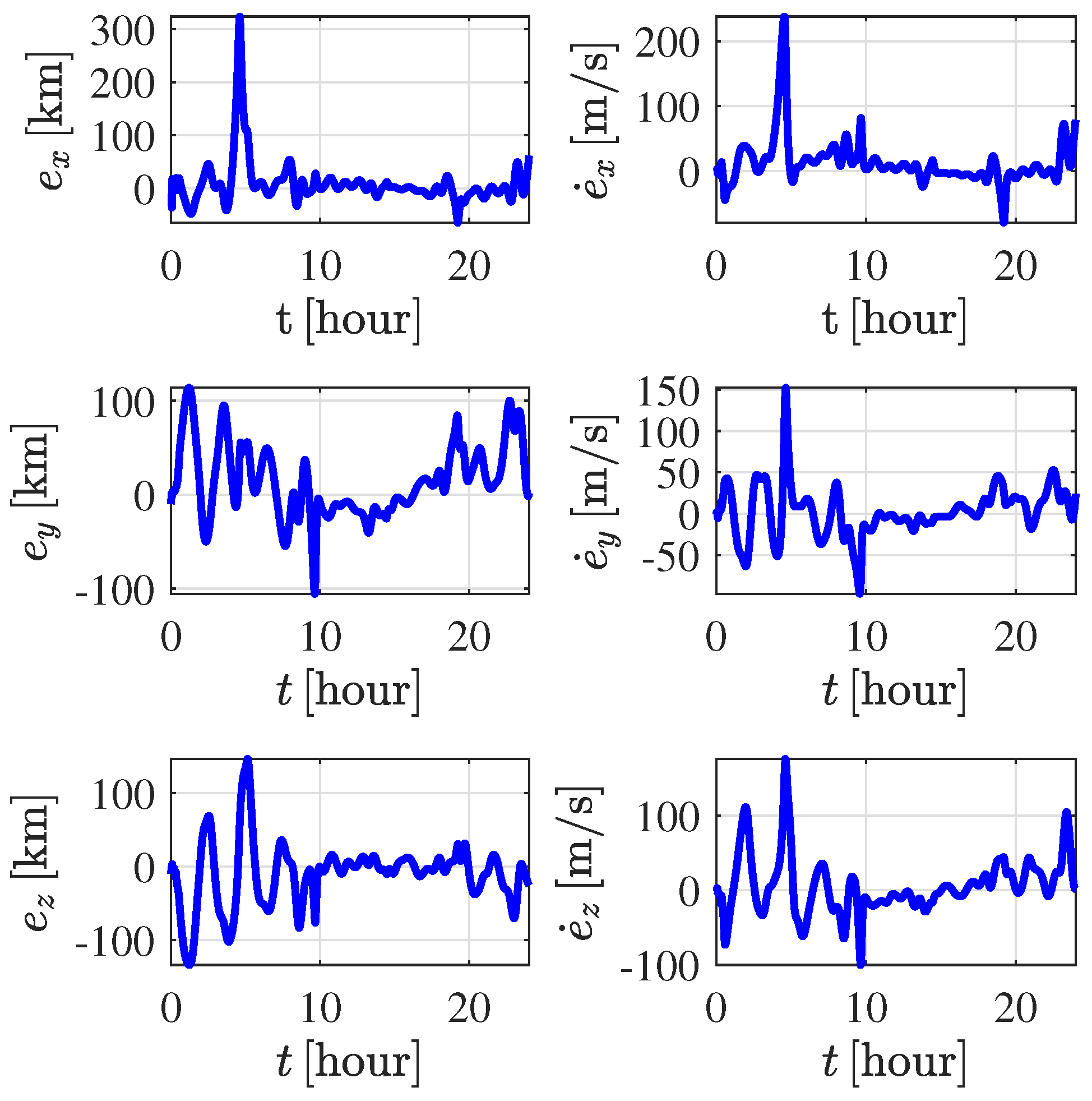
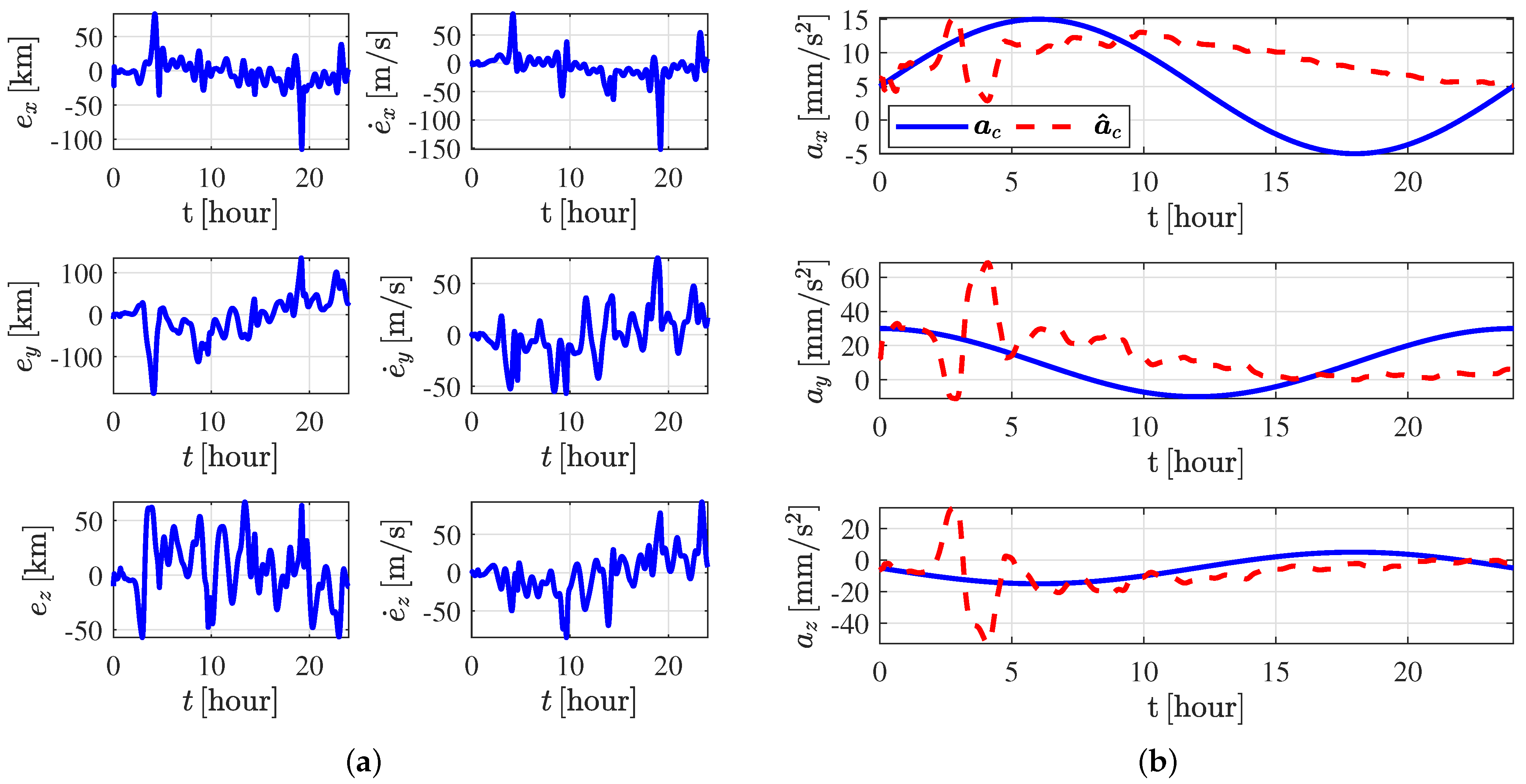
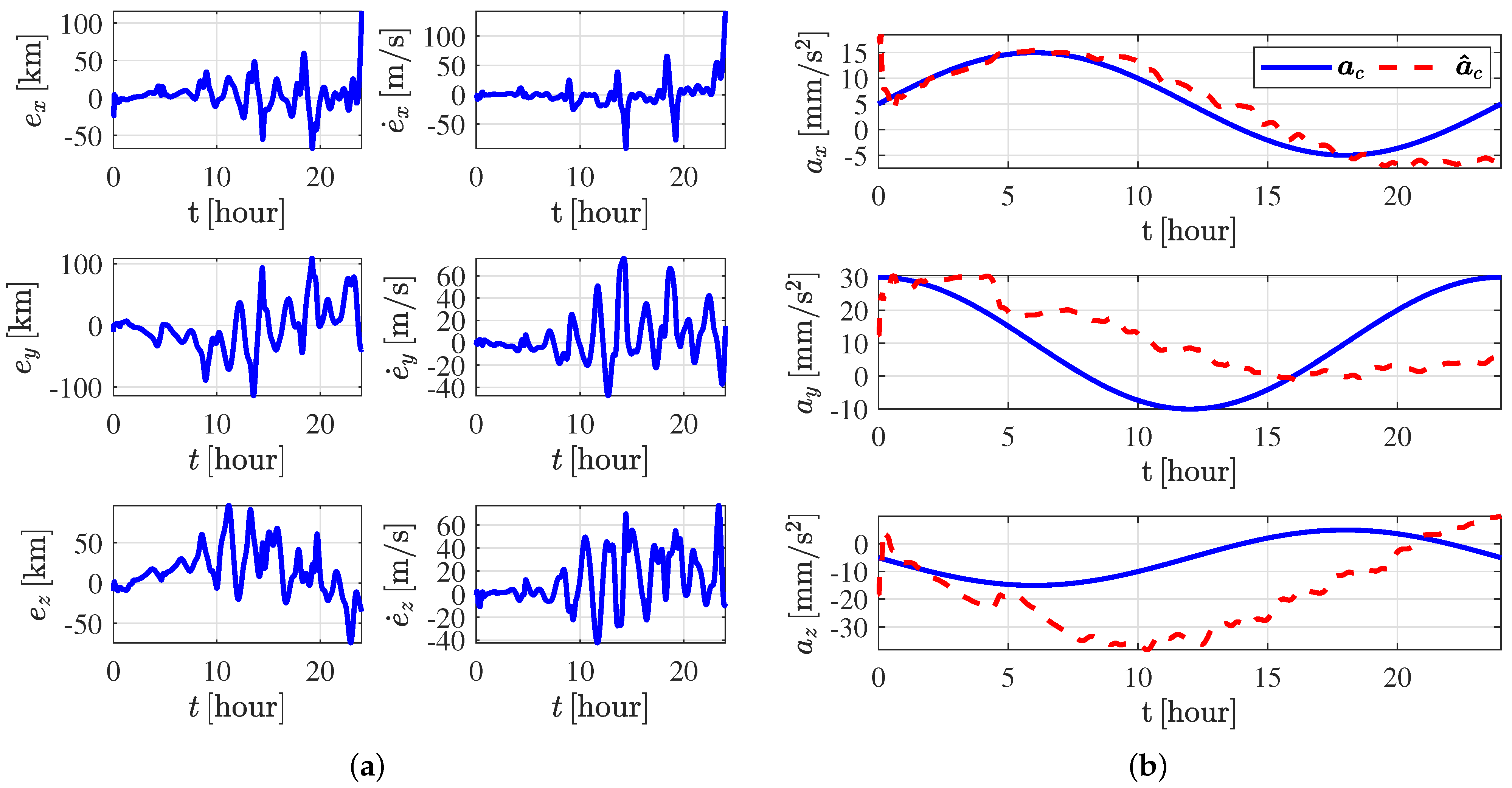
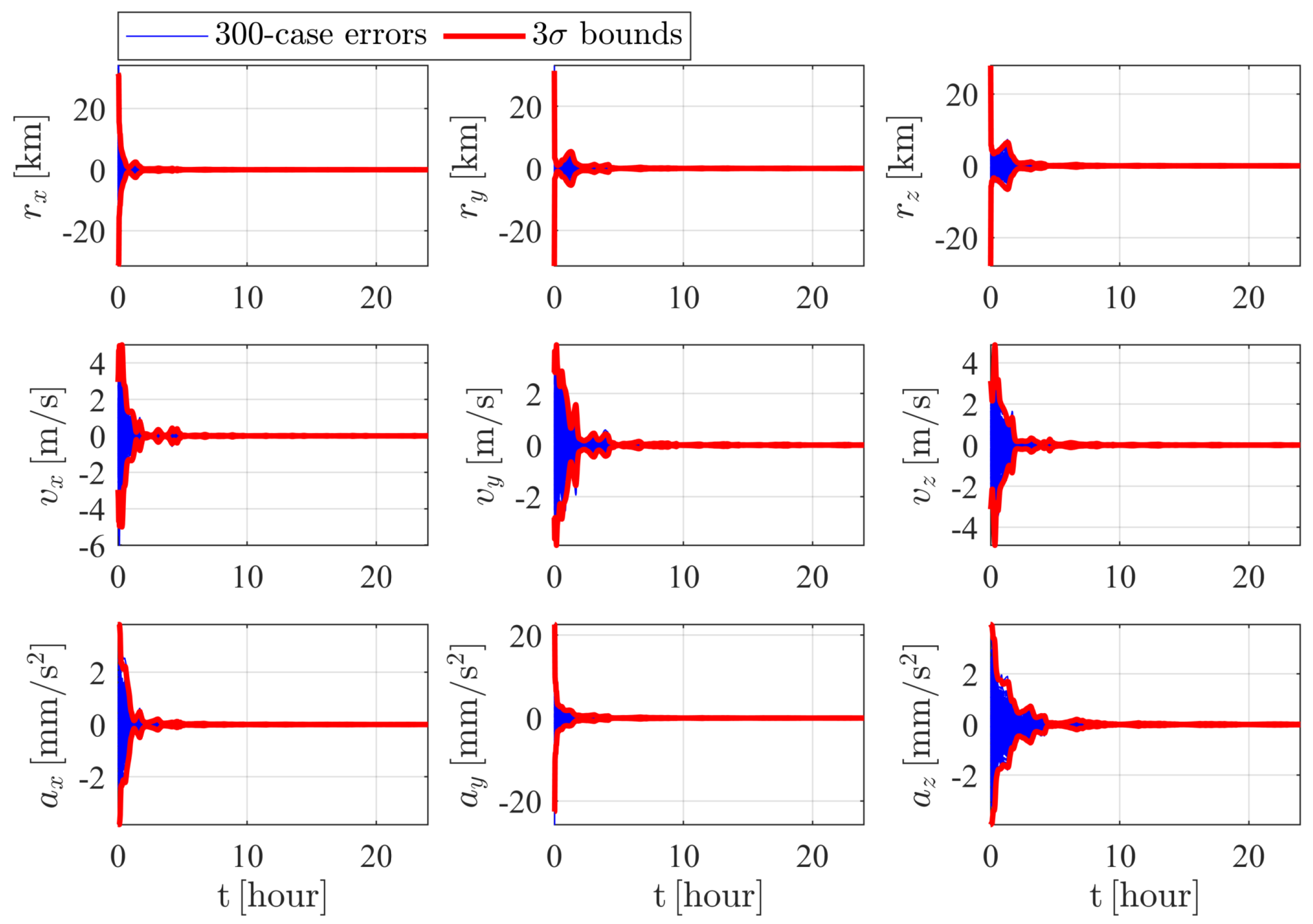
5. Performance Analysis

In this section, numerical simulations are implemented to validate the performance of the proposed method. Cases with and without maneuvers, are considered. The maneuvering case is to investigate the performance of the polynomials in compensating the unknown maneuver. Moreover, the non-maneuvering case is used to test whether the noise-induced errors is identified as the unknown maneuver by polynomial models.

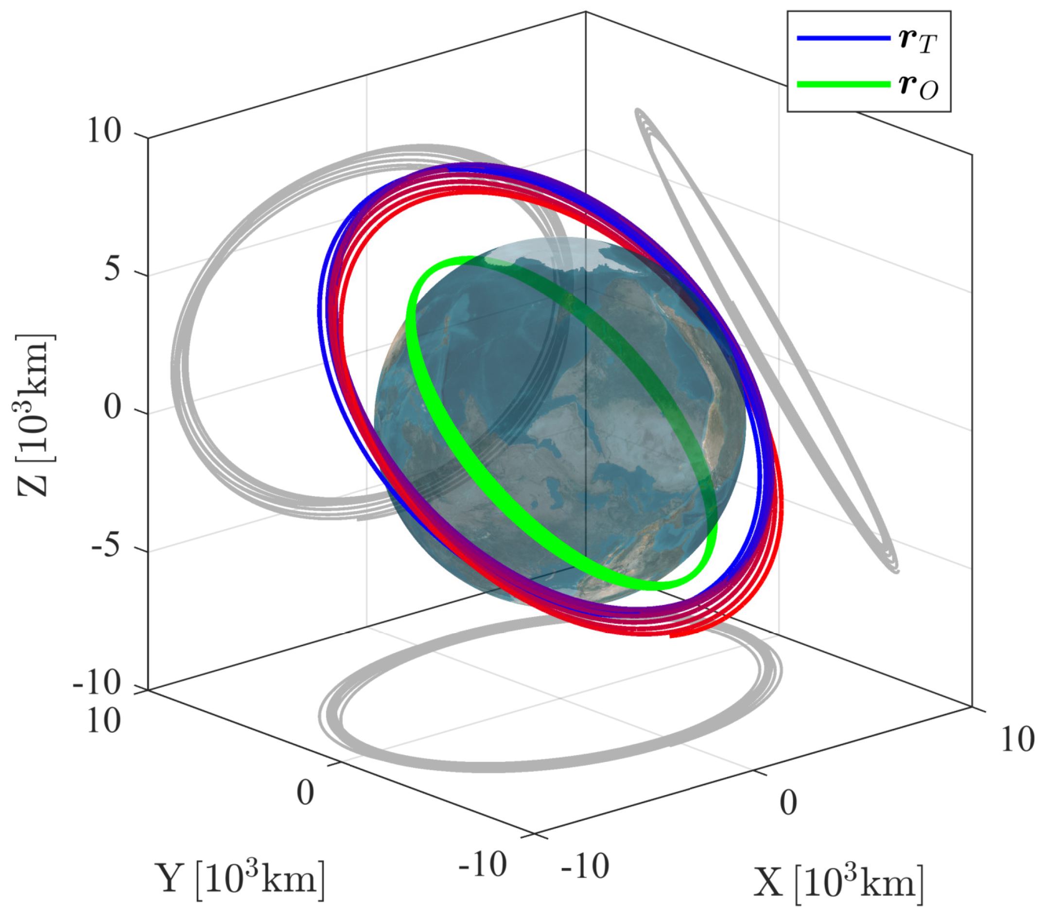
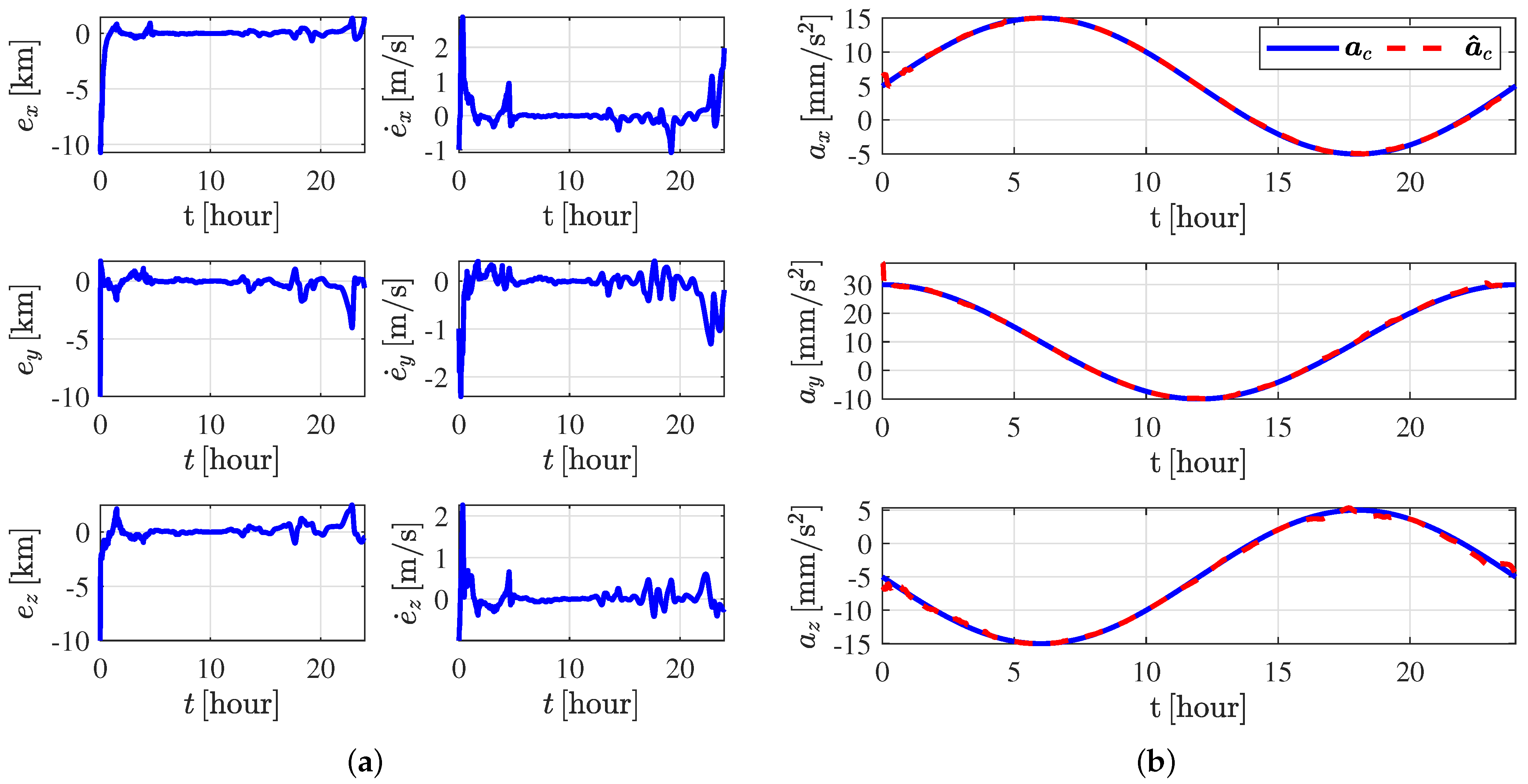
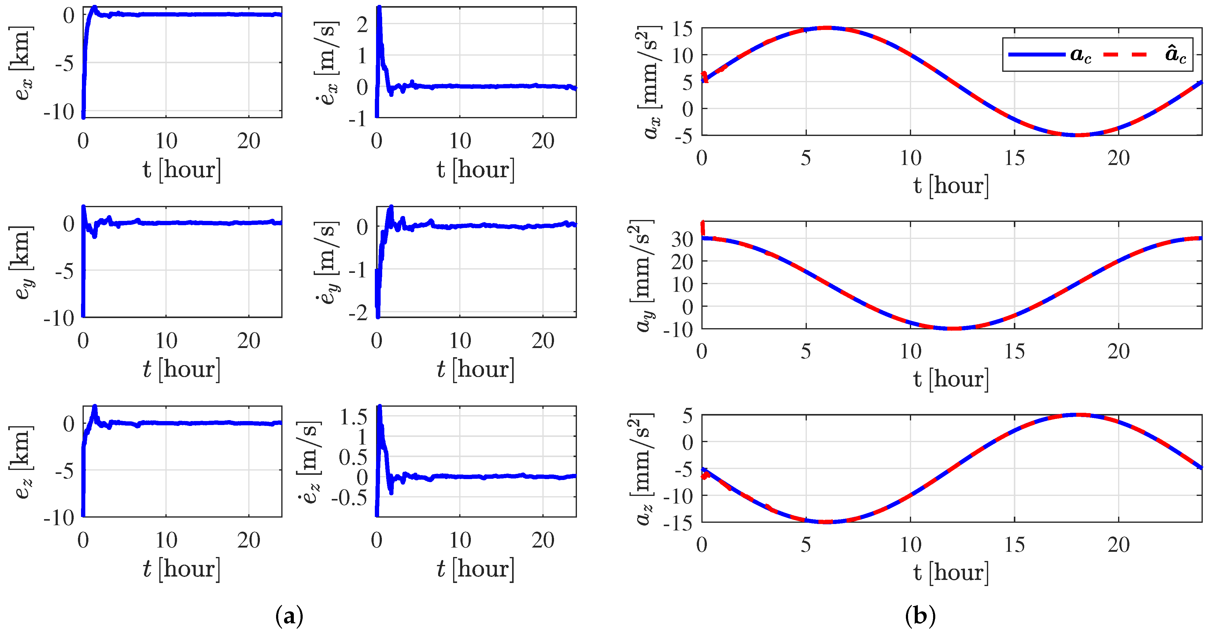
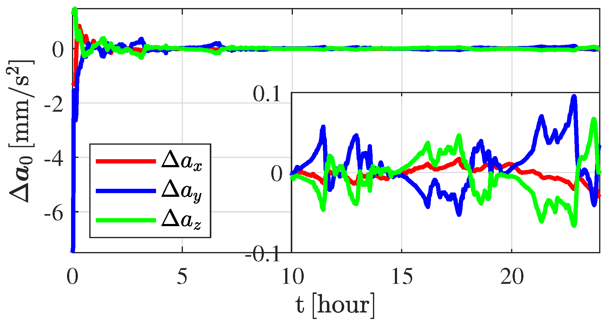
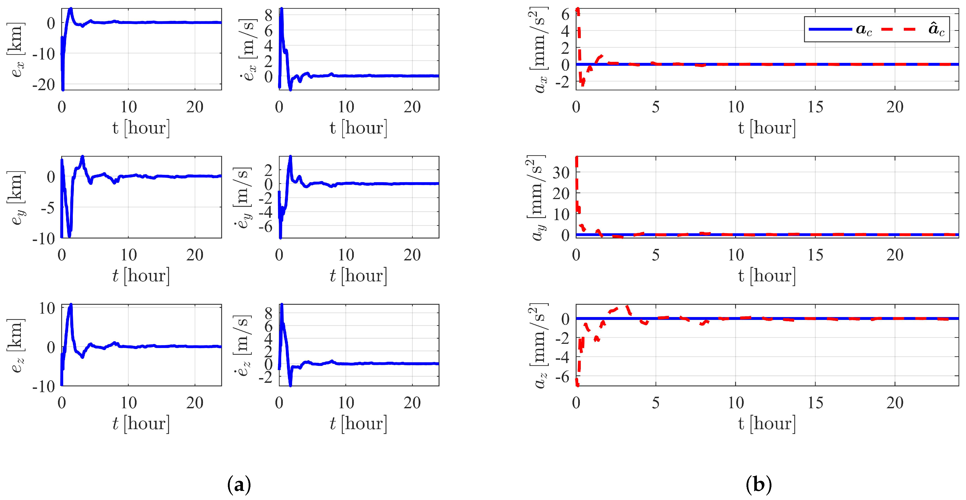
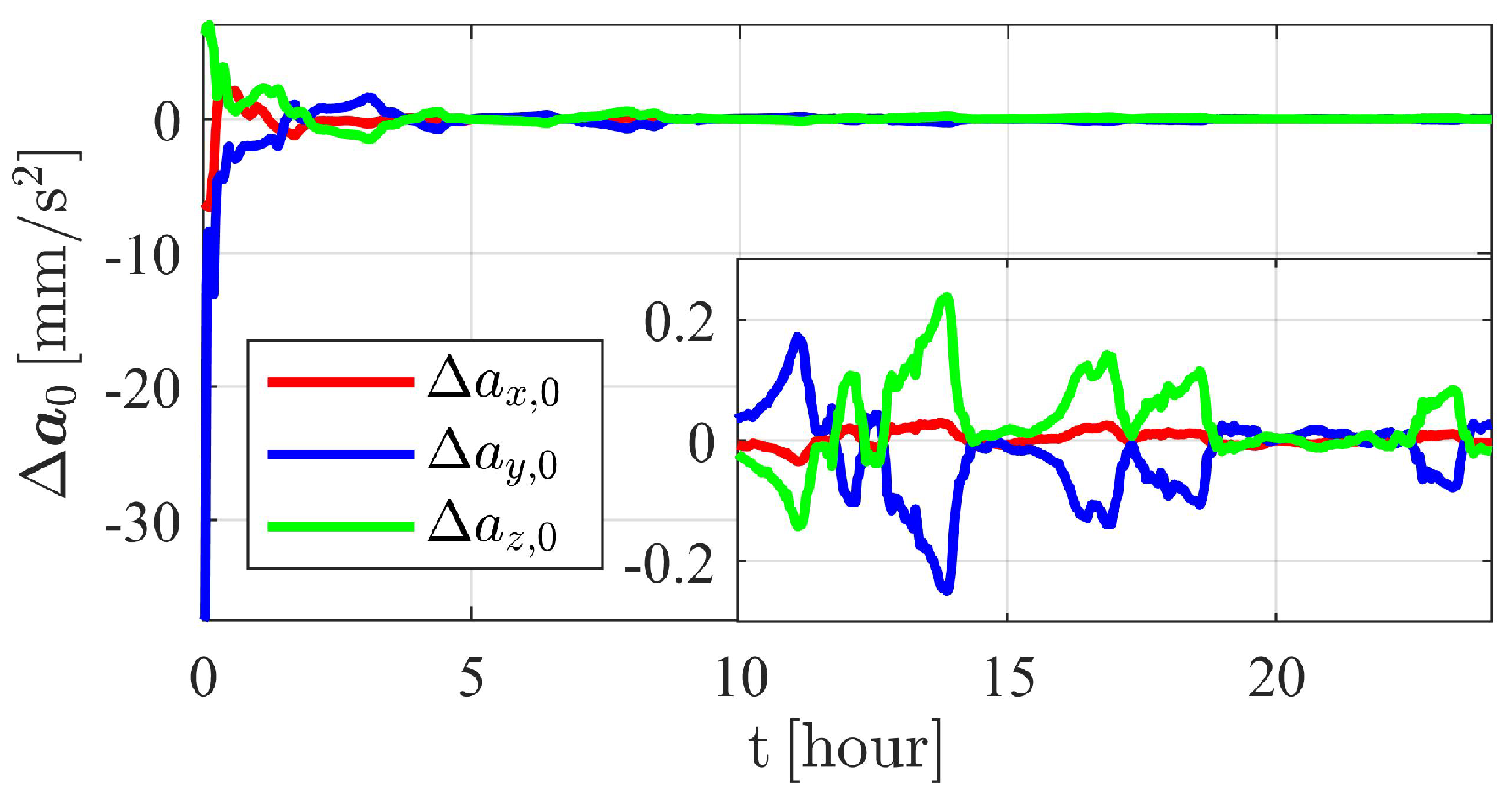
5.1. Maneuvering Case

The nominal orbit elements of the target and observer are the same as those in Section 4.2, which are listed in Table 1. The maneuvering acceleration of the target is set as: The maneuver acceleration of the target is set as:

$${\mathit{a}}_c=\left[\begin{array}{c}{a}_x\hfill \\ a_y\hfill \\ a_z\hfill \end{array}\right]=\left[\begin{array}{c}5+10sin\left(\frac{t}{T}\pi \right)\\ 10+20cos\left(\frac{t}{T}\pi \right)\\ -5-10sin\left(\frac{t}{T}\pi \right)\end{array}\right]\mathrm{mm}/{\mathrm{s}}^2$$

(25)

where $T=43,200$ s is the normalized time.

The total navigation period is set to be 24 h, with a 100 s measurement interval. The initial position and velocity estimated errors are given as 10 km and 1 m/s per axis. The standard derivations (STD) of the inter-spacecraft range and the velocity measurement are set to be 1 m and 1 mm/s, respectively.

Obviously, it is not possible for a polynomial to approximate the sines and cosines on the entire numerical axis. The polynomial is used to represented the ‘unknown’ maneuver in a particular time interval. For time epochs that extend this interval, the OD process can continue by reinitialize a polynomial representation.

The simulation results are shown in Figure 6, Figure 7, Figure 8, Figure 9, Figure 10 and Figure 11. The OD results of the case without using the polynomials are illustrated in Figure 6. The results using the zeroth-order polynomials, the first-order polynomials, the sixth-order polynomials and the eighth-order polynomials are shown in Figure 7, Figure 8, Figure 9 and Figure 10, respectively.

It can be seen that the case without using polynomials has the largest estimated errors, with the position errors larger than 300 km and the velocity larger than 200 m/s. For case using the zeroth-order polynomials and the first-order polynomials, the unknown maneuvers are not approximated accurately and their navigation performances are poor. As shown in Figure 7 and Figure 8, the position estimated errors are around 50 km.

As illustrated in Figure 9, the navigation performance using the sixth-order polynomials is greatly enhanced compared with the above three cases. The position estimated errors in the first 15 h are less than 2 km while in the last 4 h the position errors are around 5 km. It is because the approximation accuracy in the last few hours degrades. As shown in Figure 9b, the unknown acceleration in the first 20 h are fitted well by the sixth-order polynomials. However, for the maneuvering acceleration along z-axis, the fitting errors are obvious when $t>20$ h, which makes the corresponding estimation errors become larger.

As shown in Figure 10, the eighth-order polynomials can well fit the unknown maneuver. The position and velocity estimated errors are illustrated in Figure 10a and the maneuver estimated errors are shown in Figure 11. The state estimated errors converge after 2 h observation. The unknown maneuver estimated errors converge within 1 h, which is faster than the position and velocity state. It can be found that the eighth-order polynomials can provide accurate OD solutions with the position estimated errors no more than 1 km. What’s more, as shown in Figure 11, the maneuver estimated errors are smaller than 0.1 mm/s².

To further compare the OD accuracy using different orders of polynomials, the Root Mean Squared Error (RMSE) of each case is listed

Table 2. Estimated RMSE of different cases.

	Position (km)			Velocity (m/s)
	$\mathit{x}$	$\mathit{y}$	$\mathit{z}$	$\mathit{x}$	$\mathit{y}$	$\mathit{z}$
Case without polynomials	42.9745	41.0717	45.2176	37.5253	29.8473	38.3986
First-order polynomials	18.7515	38.5372	33.1376	21.1524	22.7494	25.2830
Sixth-order polynomials	0.8887	0.7339	0.6962	0.3923	0.3587	0.2428
Eighth-order polynomials	0.8247	0.4135	0.4614	0.2751	0.2305	0.2104
Ninth-order polynomials	0.8572	0.4014	0.4641	0.2774	0.2375	0.2028
Tenth-order polynomials	0.8572	0.4014	0.4640	0.2774	0.2375	0.2028

. The smaller the RMSE, the better the OD performance. The case without the maneuvering compensation has the largest RMSE, with the position and velocity estimated RMSEs larger than 40 km and 30 m/s, respectively. The OD accuracy of the method using the first-order polynomials are close to that of the method using the zeroth-order polynomials. The position and velocity RMSEs of the methods using the sixth-order and eighth-order polynomials are better than 1 km and 0.5 m/s. The eighth-order polynomials have the smallest RMSEs. The higher-order polynomials have more accurate OD solutions, while incur higher burden.

What’s more, the time consumption of the one-step run time using different polynomials are shown in

Table 3. Comparison of the one-step run time.

One-Step Run Time (s)	Mean Value	Maximum	Minimum
Zeroth-order polynomials	0.0405	0.1731	0.0214
First-order polynomials	0.0495	0.2083	0.0261
Sixth-order polynomials	0.1143	0.3482	0.0598
Eighth-order polynomials	0.1405	0.5584	0.0733
Ninth-order polynomials	0.1852	0.6222	0.0841
Tenth-order polynomials	0.2015	0.6507	0.0911

. It can be that though increasing polynomial order enhances the performance, it brings higher computational burden. Thus, a tradeoff between the OD accuracy and the time cost should be considered. As shown in Table 2, compared with the eighth-order polynomials, the OD accuracy enhancement of the ninth-order polynomials and the tenth-order polynomials are not obvious. However, the computational overhead of the ninth-order polynomials and the tenth-order polynomials are much larger than the eighth-order polynomials. Thus, in this case, the eighth-order polynomial is the best choice. Thus, for a real-world application, it is necessary to do some numerical simulations to make a tradeoff between the accuracy and the cost.

Finally, the Monte Carlo (MC) simulations are performed to validate the OD accuracy of the method using eighth-order polynomials under initial estimation uncertainty. The estimation errors of 300 runs of MC simulations are shown in Figure 12. The 3-STD ($3\sigma$) bounds of the estimation errors are depicted by the red lines in Figure 12 and the detailed values of the STDs are listed in

Table 4. Convergence ratios of the method using the eighth-order polynomials.

		x-Axis	y-Axis	z-Axis
Position (km)	Initial STDs	10.5165	10.4778	9.2985
	Final STDs	0.0042	0.0045	0.0013
	Convergence ratio, %	99.9597	99.9562	99.9850
Velocity (m/s)	Initial STDs	0.9874	0.9388	1.0395
	Final STDs	0.0048	0.0013	0.0006
	Convergence ratio, %	99.5121	99.8581	99.9360
Acceleration (mm/s2)	Initial STDs	1.2727	7.5294	1.3175
	Final STDs	0.0007	0.0026	0.0021
	Convergence ratio, %	99.9424	99.9652	99.8353

. The convergence ratios, which can be calculated using Equation (30), are also shown in Table 4. It can be seen that, the convergence ratios of the method using eighth-order polynomials are higher than 99.8%.

$$\mathrm{convergence}\mathrm{ratio}=\frac{\mathrm{Initial}\mathrm{STDs}-\mathrm{Final}\mathrm{STDs}}{\mathrm{Initial}\mathrm{STDs}}\times 100\%$$

(26)

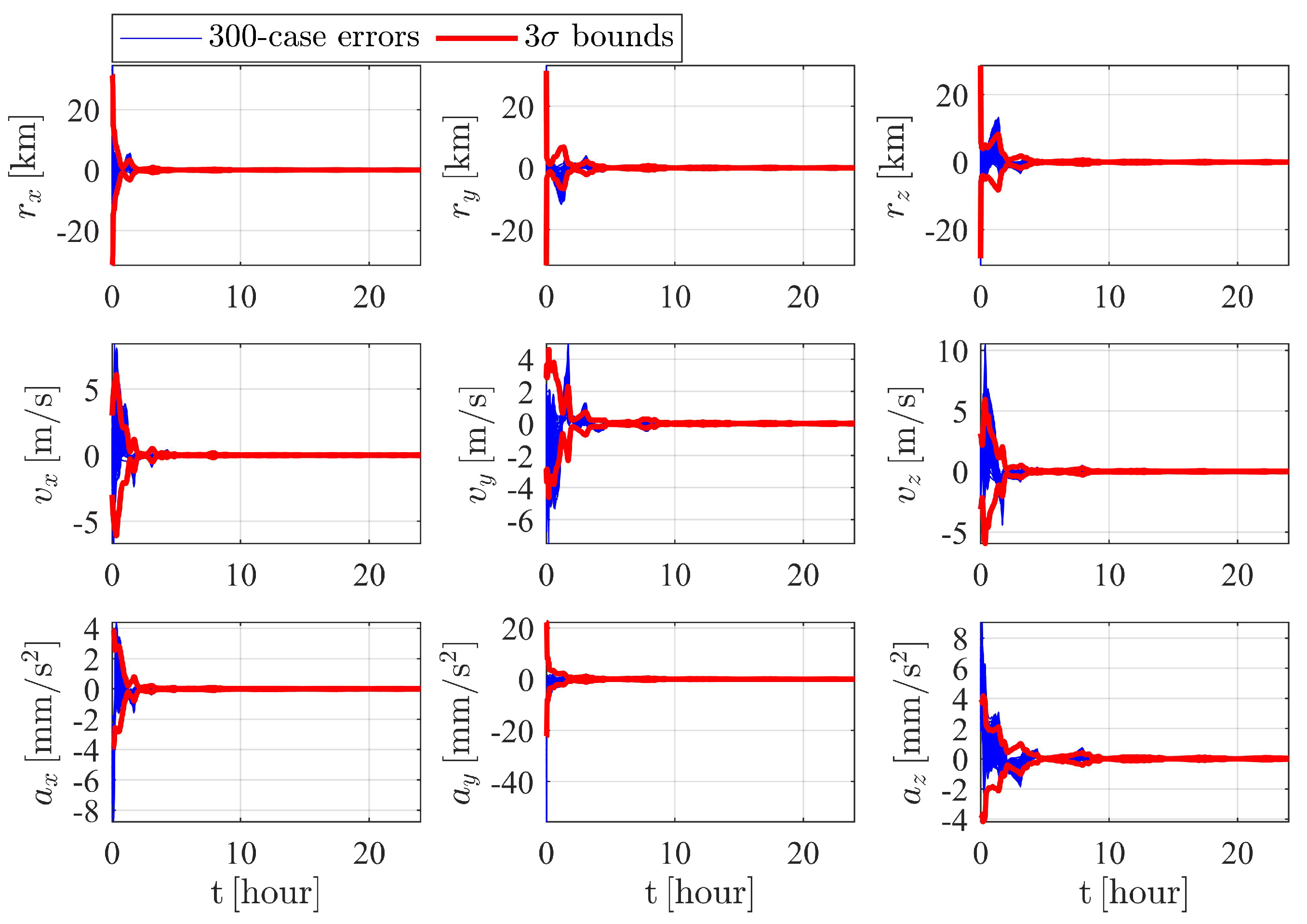
5.2. Non-Maneuvering Case

In this subsection, a non-maneuvering case is simulated. The defect of the previous maneuvering tracking methods is that they rely on priori information or predefined models about the unknown maneuver. Their performances degrade in the non-maneuvering period as the noise-induced errors are usually identified as the unknown maneuver and are compensated by the filter. Therefore, in the following, the non-maneuvering case is tested to show the advantages of not relying on priori information.

The method using the eighth-order polynomials is used to solve the OD problem. The OD results are illustrated in Figure 13 and Figure 14. It can be seen that the estimation errors converge to zero after around 5-h observation. The maneuver estimated errors are around 0.1 mm/s², indicating that the measurement noised-induced errors are not wrongly compensated by the polynomials.

Moreover, MC simulations are implemented to show the accuracies of the proposed method in solving the non-maneuvering OD problem. The corresponding results are shown in Figure 15 and

Table 5. Convergence ratios of the non-maneuvering case.

		x-Axis	y-Axis	z-Axis
Position (km)	Initial STDs	10.5201	10.5118	9.5303
	Final STDs	0.0121	0.0197	0.0123
	Convergence ratio, %	99.8846	99.8116	99.8706
Velocity (m/s)	Initial STDs	0.9956	0.9425	1.0383
	Final STDs	0.0077	0.0059	0.0061
	Convergence ratio, %	99.2178	99.3675	99.4073
Acceleration (mm/s2)	Initial STDs	1.2749	7.3985	1.3145
	Final STDs	0.0021	0.0110	0.0088
	Convergence ratio, %	99.8303	99.8500	99.3248

. It can be seen that the convergence ratios of the position, the velocity and the unknown maneuvering acceleration are 99.8%, 99.2% and 99.3%, respectively. The convergence ratios are 0.2% lower than the maneuvering case, and no obvious performance degradation is found.

6. Conclusions

This paper proposed a polynomial representation-based method for maneuvering spacecraft orbit determination (OD). The OD performance of the proposed method is tested by applying it over different cases. Numerical simulations show that the method can well track the maneuvering spacecraft. It is found that the extended Kalman filter (EKF) using sixth-order polynomials are enough to provide valid OD solutions. Higher-order polynomials bring more accurate estimations. Moreover, the proposed method can also be applied into non-maneuvering cases and the noise-induced errors will not be wrongly compensated by the polynomial representation. In the future, the performance of the proposed method in dealing with impulsive maneuvers should be further investigated.

References

1. Cui, P.Y.; Qiao, D.; Cui, H.T.; Luan, E.J. Target selection and transfer trajectories design for exploring asteroid mission. Sci. China Technol. Sci. 2010, 53, 1150–1158. [Google Scholar] [CrossRef]
2. Yang, H.; Li, S.; Bai, X. Fast homotopy method for asteroid landing trajectory optimization using approximate initial costates. J. Guid. Control Dyn. 2019, 42, 585–597. [Google Scholar] [CrossRef]
3. Colagrossi, A.; Lavagna, M. Fault Tolerant Attitude and Orbit Determination System for Small Satellite Platforms. Aerospace 2022, 9, 46. [Google Scholar] [CrossRef]
4. Wang, Y.; Qiao, D.; Cui, P. Design of optimal impulse transfers from the Sun-Earth libration point to asteroid. Adv. Space Res. 2015, 56, 176–186. [Google Scholar] [CrossRef]
5. Pesce, V.; Silvestrini, S.; Lavagna, M. Radial basis function neural network aided adaptive extended Kalman filter for spacecraft relative navigation. Aerosp. Sci. Technol. 2020, 96, 105527. [Google Scholar] [CrossRef]
6. Cloutier, J.R.; Lin, C.F.; Yang, C. Maneuvering target tracking via smoothing and filtering through measurement concatenation. J. Guid. Control Dyn. 1993, 16, 377–384. [Google Scholar] [CrossRef]
7. Yu, S.; Wang, X.; Zhu, T. Maneuver detection methods for space objects based on dynamical model. Adv. Space Res. 2021, 68, 71–84. [Google Scholar] [CrossRef]
8. Li, X.; Qiao, D.; Jia, F. Investigation of Stable Regions of Spacecraft Motion in Binary Asteroid Systems by Terminal Condition Maps. J. Astronaut. Sci. 2021, 68, 891–915. [Google Scholar] [CrossRef]
9. Ko, H.C.; Scheeres, D.J. Tracking maneuvering satellite using thrust-fourier-coefficient event representation. J. Guid. Control Dyn. 2016, 39, 216–221. [Google Scholar] [CrossRef]
10. Jia, F.; Li, X.; Huo, Z.; Qiao, D. Mission Design of an Aperture-Synthetic Interferometer System for Space-Based Exoplanet Exploration. Space Sci. Technol. 2022, 2022, 9835234. [Google Scholar] [CrossRef]
11. Kelecy, T.; Jah, M. Detection and orbit determination of a satellite executing low thrust maneuvers. Acta Astronaut. 2010, 66, 798–809. [Google Scholar] [CrossRef]
12. Chan, Y.T.; Hu, A.G.; Plant, J.B. A Kalman Filter Based Tracking Scheme with Input Estimation. IEEE Trans. Aerosp. Electron. Syst. 1979, AES-15, 237–244. [Google Scholar] [CrossRef]
13. Zhou, X.; Cheng, Y.; Qiao, D.; Huo, Z. An adaptive surrogate model-based fast planning for swarm safe migration along halo orbit. Acta Astronaut. 2022, 194, 309–322. [Google Scholar] [CrossRef]
14. Lubey, D.P.; Scheeres, D.J.; Erwin, R.S. Maneuver Detection and Reconstruction of Station-keeping Spacecraft at GEO using the Optimal Control-Based Estimator. IFAC-PapersOnLine 2015, 48, 216–221. [Google Scholar] [CrossRef]
15. Serra, R.; Yanez, C.; Frueh, C. Tracklet-to-orbit association for maneuvering space objects using optimal control theory. Acta Astronaut. 2021, 181, 271–281. [Google Scholar] [CrossRef]
16. Tang, Y.; Wu, W.; Qiao, D.; Li, X. Effect of orbital shadow at an Earth-Moon Lagrange point on relay communication mission. Sci. China Inf. Sci. 2017, 60, 112301. [Google Scholar] [CrossRef] [Green Version]
17. Wang, Z.; Li, Z.; Wang, N.; Hoque, M.; Wang, L.; Li, R.; Zhang, Y.; Yuan, H. Real-Time Precise Orbit Determination for LEO between Kinematic and Reduced-Dynamic with Ambiguity Resolution. Aerospace 2022, 9, 25. [Google Scholar] [CrossRef]
18. Li, X.; Qiao, D.; Li, P. Bounded trajectory design and self-adaptive maintenance control near non-synchronized binary systems comprised of small irregular bodies. Acta Astronaut. 2018, 152, 768–781. [Google Scholar] [CrossRef]
19. Li, T.; Li, K.; Chen, L. New manoeuvre detection method based on historical orbital data for low Earth orbit satellites. Adv. Space Res. 2018, 62, 554–567. [Google Scholar] [CrossRef]
20. Li, X.; Qiao, D.; Chen, H. Interplanetary transfer optimization using cost function with variable coefficients. Astrodynamics 2019, 3, 173–188. [Google Scholar] [CrossRef]
21. Hough, M.E. Reentry maneuver estimation using nonlinear Markov acceleration models. J. Guid. Control Dyn. 2017, 40, 1693–1710. [Google Scholar] [CrossRef]
22. Guang, Z.; Xingzi, B.; Hanyu, Z.; Bin, L. Non-cooperative maneuvering spacecraft tracking via a variable structure estimator. Aerosp. Sci. Technol. 2018, 79, 352–363. [Google Scholar] [CrossRef]
23. Zhai, G.; Wang, Y.; Zhao, Q. Tracking the maneuvering spacecraft propelled by swing propulsion of constant magnitude. J. Syst. Eng. Electron. 2020, 31, 370–382. [Google Scholar] [CrossRef]
24. Maybeck, P.S.; Hentz, K.P. Investigation of moving-bank multiple model adaptive algorithms. J. Guid. Control Dyn. 1987, 10, 90–96. [Google Scholar] [CrossRef]
25. Lee, S.; Lee, J.; Hwang, I. Maneuvering spacecraft tracking via state-dependent adaptive estimation. J. Guid. Control Dyn. 2016, 39, 2034–2043. [Google Scholar] [CrossRef]
26. Linares, R.; Furfaro, R. Space Objects Maneuvering Detection and Prediction via Inverse Reinforcement Learning. In Proceedings of the Advanced Maui Optical and Space Surveillance, Maui, HI, USA, 19–22 September 2017; Volume 46, p. 46. [Google Scholar]
27. Wang, Y.; Bai, X.; Peng, H.; Chen, G.; Shen, D.; Blasch, E.; Sheaff, C.B. Gaussian-Binary classification for resident space object maneuver detection. Acta Astronaut. 2021, 187, 438–446. [Google Scholar] [CrossRef]
28. Peng, H.; Bai, X. Improving orbit prediction accuracy through supervised machine learning. Adv. Space Res. 2018, 61, 2628–2646. [Google Scholar] [CrossRef] [Green Version]
29. Silvestrini, S.; Lavagna, M. Neural-based predictive control for safe autonomous spacecraft relative maneuvers. J. Guid. Control. Dyn. 2021, 44, 2303–2310. [Google Scholar] [CrossRef]
30. Wu, W.; Tang, Y.; Zhang, L.; Qiao, D. Design of communication relay mission for supporting lunar-farside soft landing. Sci. China Inf. Sci. 2018, 61, 040305. [Google Scholar] [CrossRef]
31. Li, X.; Qiao, D.; Li, P. Frozen orbit design and maintenance with an application to small body exploration. Aerosp. Sci. Technol. 2019, 92, 170–180. [Google Scholar] [CrossRef]
32. Wang, Y.; Zhang, Y.; Qiao, D.; Mao, Q.; Jiang, J. Transfer to near-Earth asteroids from a lunar orbit via Earth flyby and direct escaping trajectories. Acta Astronaut. 2017, 133, 177–184. [Google Scholar] [CrossRef]
33. Li, X.; Qiao, D.; Barucci, M.A. Analysis of equilibria in the doubly synchronous binary asteroid systems concerned with non-spherical shape. Astrodynamics 2018, 2, 133–146. [Google Scholar] [CrossRef]
34. Qin, T.; Macdonald, M.; Qiao, D. Fully Decentralized Cooperative Navigation for Spacecraft Constellations. IEEE Trans. Aerosp. Electron. Syst. 2021, 57, 2383–2394. [Google Scholar] [CrossRef]
35. Qin, T.; Qiao, D.; Macdonald, M. Relative orbit determination using only intersatellite range measurements. J. Guid. Control Dyn. 2019, 42, 703–710. [Google Scholar] [CrossRef]
36. Qin, T.; Qiao, D.; Macdonald, M. Relative orbit determination for unconnected spacecraft within a constellation. J. Guid. Control Dyn. 2021, 44, 614–621. [Google Scholar] [CrossRef]
37. Luo, Y.; Qin, T.; Zhou, X. Observability Analysis and Improvement Approach for Cooperative Optical Orbit Determination. Aerospace 2022, 9, 166. [Google Scholar] [CrossRef]
Figure 1. Illustration of the nominal orbits of the target and the observer. The orbit is colored by red at the beginning and gradually changes to blue at the end. The grey lines represent the projection of the nominal orbit.
Aerospace 09 00257 g001
Figure 2. Observability analysis results of the zeroth-order polynomial.
Aerospace 09 00257 g002
Figure 3. Observability analysis results of the first-order polynomial.
Aerospace 09 00257 g003
Figure 4. Observability analysis results of the sixth-order polynomial.
Aerospace 09 00257 g004
Figure 5. Observability analysis results of the eighth-order polynomial.
Aerospace 09 00257 g005
Figure 6. OD results without using the polynomials. The blue lines represent the estimated errors.
Aerospace 09 00257 g006
Figure 7. OD results using the zeroth-order polynomials. (a) State estimated errors. (b) Maneuver estimated comparison (the blue lines denote the real maneuvering acceleration and the red dashed lines represent the estimated maneuvering acceleration).
Aerospace 09 00257 g007
Figure 8. OD results using the first-order polynomials. (a) State estimated errors. (b) Maneuver estimated comparison (the blue lines denote the real maneuvering acceleration and the red dashed lines represent the estimated maneuvering acceleration).
Aerospace 09 00257 g008
Figure 9. OD results using the sixth-order polynomials. (a) State estimated errors. (b) Maneuver estimated comparison (the blue lines denote the real maneuvering acceleration and the red dashed lines represent the estimated maneuvering acceleration).
Aerospace 09 00257 g009
Figure 10. OD results using the eighth-order polynomials. (a) State estimated errors. (b) Maneuver estimated comparison (the blue lines denote the real maneuvering acceleration and the red dashed lines represent the estimated maneuvering acceleration).
Aerospace 09 00257 g010
Figure 11. Maneuver estimated errors using the eighth-order polynomials.
Aerospace 09 00257 g011
Figure 12. Monte Carlo simulations results using the eighth-order polynomials.
Aerospace 09 00257 g012
Figure 13. OD results of the non-maneuvering case. (a) State estimated errors. (b) Maneuver estimated comparison (the blue lines denote the real maneuvering acceleration and the red dashed lines represent the estimated maneuvering acceleration).
Aerospace 09 00257 g013
Figure 14. Maneuver estimated errors of the non-maneuvering case.
Aerospace 09 00257 g014
Figure 15. Monte Carlo simulations results of the non-maneuvering case.
Aerospace 09 00257 g015