Article

Effect of Stagger on Low-Speed Performance of Busemann Biplane Airfoil

1
Department of Aerospace Engineering, National Defense Academy of Japan, Yokosuka 239-8686, Japan
2
Formerly Japan Aerospace Exploration Agency, Tokyo 182-8522, Japan
*
Author to whom correspondence should be addressed.
Aerospace 2022, 9(4), 197; https://doi.org/10.3390/aerospace9040197
Submission received: 11 March 2022 / Revised: 29 March 2022 / Accepted: 4 April 2022 / Published: 6 April 2022
(This article belongs to the Section Aeronautics)

Abstract

:
In this study, the low-speed performances of the Busemann biplane were clarified, focusing on the relative contributions of the upper and lower elements to the total aerodynamic characteristics of the biplane. Also, the effects of the staggered biplane, which changes the horizontal distance between two wings in a biplane configuration, were investigated by balance measurements and numerical simulations. The flow velocity was 15 m/s, and the Reynolds number based on the airfoil chord length was 2.1 × 10⁵. In the tests of the integrated biplane wing, the attack angles of the wing elements were varied by a balance system and turntable, which were set in the wind tunnel sidewall. The results show that the lower element generated most of the lift and drag of the Busemann biplane (or the baseline biplane model with no stagger) at high angles of attack. At angles above 20 deg, the contribution of the lower element to total aerodynamic characteristics is almost constant, with 95% of the total lift and 88% of the total drag. The total lift and drag of the baseline model were smaller than the sum of the individual elements that were treated as a single configuration. The increments of lift and drag due to the stagger effects were confirmed, especially at high angles of attack. When the stagger value increases, the high-pressure area near the leading edge of the lower surface of the upper element also increases, which increases the lift and drag of the up-per element. This is the main reason for the increments of total lift and drag of the biplane model. The stagger effects also prevented the leading-edge separation of the lower element in the biplane configuration and increased the lift slopes of the biplane model.

1. Introduction

In recent years, many projects and studies have been conducted to develop supersonic transport aircraft [1,2,3]. For a supersonic flight to be accepted by society, it is necessary to solve the problems of the flight path, fuel consumption, and the noise caused by sonic booms. The Busemann biplane has been proposed to solve the drag and sonic boom problems. Wind tunnel tests and numerical simulations have been carried out to clarify the characteristics of the Busemann biplane [4,5,6,7,8]. The Busemann biplane is a diamond-shaped airfoil (or double-wedge airfoil) that is split and inverted with respect to the chord. Previous studies show that a Busemann biplane reduces wave drag more than 80% compared to a diamond wing of similar volume at a design Mach number [4,5]. In addition, three-dimensional tapered wings, wing-body shapes, and twin-body fuselage configurations are also being investigated [9,10,11,12].
Studies of the Busemann biplane have found attractive performance at cruising speeds. However, there are several problems that need to be solved to realize the Busemann biplane [5]. The first problem is the choked flow between the wing elements in the transonic region and near the design Mach number, which dramatically increases the total drag. The second problem is hysteresis due to the different starting Mach numbers, which can cancel the shock waves between the wing elements at the flow acceleration and deceleration. To solve the above problems, the morphing wing [4], leading and trailing edge flaps [13], and the stagger approach [14,15], which changes the horizontal distance between two wings in a biplane configuration, have been proposed. Steady computational fluid dynamics (CFD) analysis by Patidar [14] have shown that Busemann biplanes with a stagger of ≥0.2 times the wing chord length in the transonic regime could avoid choked flow and significantly reduce the total drag. The results also show impressive improvement in the lift-to-drag ratio of the biplanes. Ma et al. [15] analyzed the unsteady numerical simulations, which showed that staggered wings could also avoid hysteresis problems, and proposed a method of changing the stagger with flight speed, which resulted in higher performance than baseline and diamond wing models. The previous studies of staggered Busemann biplanes focused on the aerodynamic characteristics in the transonic and supersonic regimes. However, the effect of stagger on the low-speed performance of the Busemann biplane remains unclear. It is necessary to clarify the low-speed characteristics, which are essential during aircraft take-off and landing.
In a previous study at low-speed flow, Kuratani et al. [16] investigated the aerodynamic characteristics of a Busemann biplane by wind tunnel experiments and CFD simulations. Their results show that the lower wing generates most of the biplane’s total lift at high angles of attack. To keep the thin wing elements in their positions, a wing tip plate was attached to the biplane model. The experimental results agreed well with the three-dimensional CFD due to the effects of the wing tip plates and the flat plate installed to eliminate the boundary layer development from the wind tunnel outlet. In another study, Kashitani et al. [17] estimated the two-dimensional lift coefficient from the smoke line pattern around the Busemann biplane. The experiments were carried out at relatively small angles of attack due to the instability of the smoke line at high angles of attack. The results show that the flow separated from the upper element at small angles of attack. At 5 deg, the flow is reattached around 0.3c from the leading edge. When the angle of attack increases, large-scale separation is observed. Due to the experimental setting, the flow field between the biplane element remains unclear. Also, further investigations of the contribution of the lower and upper elements to the total performance of the Busemann biplane are required.
At a low-speed regime, Jones et al. [18] studied a biplane made with flat plate elements. Their results show that the stall angle of the biplane wing is larger than that of a single wing. The reason for this is that the flow between the wing elements is compressed and delays the lower wing’s flow separation. For a biplane with a 0.5-chord stagger, the gap between the wing elements with a 0.85 chord length was most effective for increasing the stall angle from 15 to 25 deg and increasing the maximum lift coefficient from 0.79 to 0.97. However, the stagger effects on Busemann biplanes, which have thin wing elements with an inverted camber, have not been fully investigated. Due to the staggered biplane configuration, the flow separation and the flow interference between not only the upper and lower elements but also between the front and rear elements are critical to the staggered biplane performances.
In this study, the low-speed performances of the Busemann biplane were clarified, focusing on the relative contributions of upper and lower elements to the total aerodynamic characteristics of the biplane. Also, the effects of the staggered biplane were investigated by balance measurements and numerical simulations. The flow interferences between the biplane elements (upper and lower wings) were also studied by testing the biplane elements as a single configuration.

2. Experimental Setup

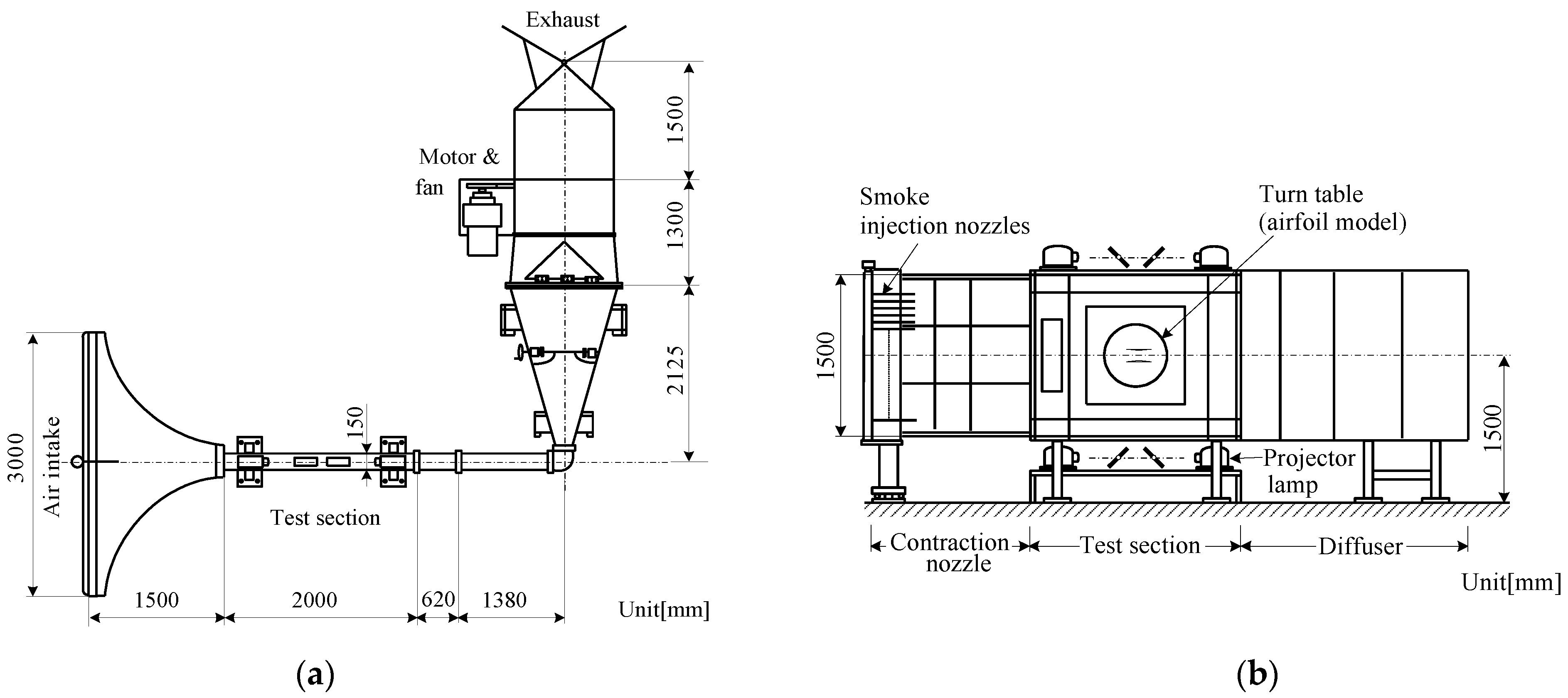
2.1. Low-Speed Wind Tunnel

Figure 1 shows an overview of the low-speed wind tunnel used in this study. The wind tunnel is a suction type, with a test section of 2000 mm length × 150 mm width × 1500 mm height. The maximum flow velocity is 26 m/s. The wind tunnel is equipped with a smoke generator (SC-3, Kanto Chemical Co., Inc., Tokyo, Japan), which enables visualization of the flow field around the test model.

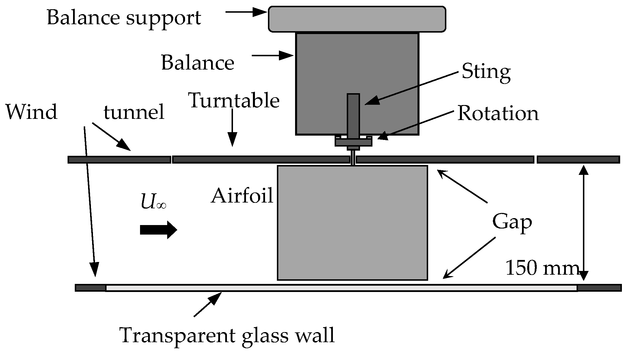
2.2. Balance Measurement System
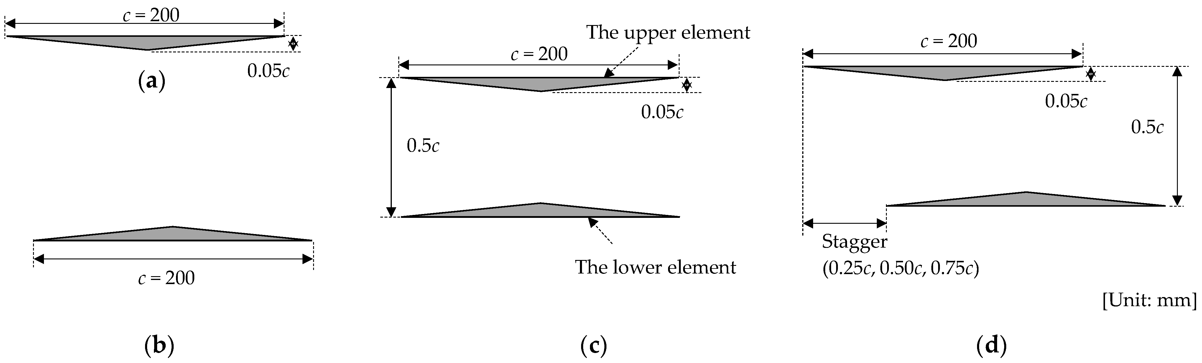
In the experiments, the aerodynamic forces acting on the model were measured using a three-component force balance system (ML-3FM2, Izumi Seiki Co., Ltd. Ehime, Japan). The balance enables adjustment of the angle of the model with a resolution of 0.1 deg. The measurable range of drag and lift of the balance is ±20 N.
Figure 2 shows the setup in the test section. In this study, the models were set up as follows to measure the aerodynamic forces acting on each element of the Busemann biplane separately, which is unclear from previous studies. For the biplane experiments, the model’s angle was adjusted by the balance system and a turntable set in the wind tunnel wall. The unmeasured wing element was fixed to the turntable. The gap between the model and the wind tunnel wall was adjusted to allow two-dimensional measurements. The gap was determined from the displacement thickness of the boundary layer on the wind tunnel walls, where the typical length is the distance from the end of the wind tunnel measurement section to the model [19,20]. In the experiments with Re = 2.1 × 10⁵, the gap was set to 1.5 mm from the wind tunnel walls. The data obtained by the balance were recorded by a data acquisition system (KEYENCE, NR-500). In this study, the balance resolutions were 0.0025 N for both lift and drag measurements.
The wind tunnel correction must be applied for two-dimensional flow testing to consider free air condition [21,22]. Under the conditions of the tests (M < 0.1, Re = 2.1 × 10⁵), the model chord length (c = 200 mm) was sufficiently small compared to the height of the test section (h = 1500 mm) [23]. In a previous study, the wind tunnel corrections for similar experimental conditions were less than 1% of the measured results [17]. Therefore, no two-dimensional wind tunnel correction was applied to the experimental results in this study.

2.3. Test Model

Figure 3 shows an overview of the experimental models used in this study. The models were made of acrylic, with a chord length c of 200 mm, a wing thickness t of 10 mm (t/c = 0.05), and a spacing between wing elements G of 100 mm (G/c = 0.5). The dimensions of the model were calculated at a design cruising Mach number of 1.7 [4]. In the single-wing tests, a single upper element and a single lower element, Figure 3a,b, were applied. In the biplane tests, the baseline model (no stagger) and three staggered models, Figure 3c,d, were applied. The upper element was set forward for the staggered biplane, and stagger values of 0.25c, 0.50c, and 0.75c were applied. Previous studies have shown that a forward placement of the upper wing has better performance than a rearward placement of the upper wing [24,25]. As the wing was thin, a sting balance with a diameter of 6 mm was inserted into the center of the wing model.

2.4. Experimental Conditions

Table 1 shows the experimental conditions in this study. The wind tunnel tests were carried out at a flow velocity U of 15 m/s and a Reynolds number Re of 2.1 × 10⁵ based on the wing chord length. The angles of attack were varied from −30 to 30 deg. A three-component balance was used for the aerodynamic measurements. The measurement time was 20 s with 5-Hz sampling. The time average values of the obtained data were used to determine the aerodynamic forces. Each experiment was conducted four times, and the average value was taken as the measurement result. This paper discusses the results in terms of lift and drag coefficients.
First, experiments were carried out with the single NACA0012 airfoil for evaluation of the two-dimensional results and comparison with the results in previous experimental studies [26,27,28].
Next, the aerodynamic characteristics of individual single elements were clarified.
Then, the total aerodynamic performance (total drag and lift coefficient) of the baseline model and the staggered models were investigated by measuring the forces acting on each element in the biplane configuration. The reference length is defined as the chord length c of a single element. The total aerodynamic coefficients of the biplane are defined by the sum of the elements in the biplane configuration, as shown in Equations (1) and (2) below.
C d _ T o t a l = C d ( L o w e r _ B i p l a n e ) + C d ( U p p e r _ B i p l a n e )
C l _ T o t a l = C l ( L o w e r _ B i p l a n e ) + C l ( U p p e r _ B i p l a n e )
where Cd_Total and Cl_Total are the total drag and total lift coefficient of the biplane configuration models, respectively, and Cd(Upper_Biplane), Cd(Lower_Biplane), Cl(Upper_Biplane), and Cl(Lower_Biplane) are the drag coefficient of the upper element, the drag coefficient of the lower element, the lift coefficient of the upper element, and the lift coefficient of the lower element in biplane configuration, respectively.

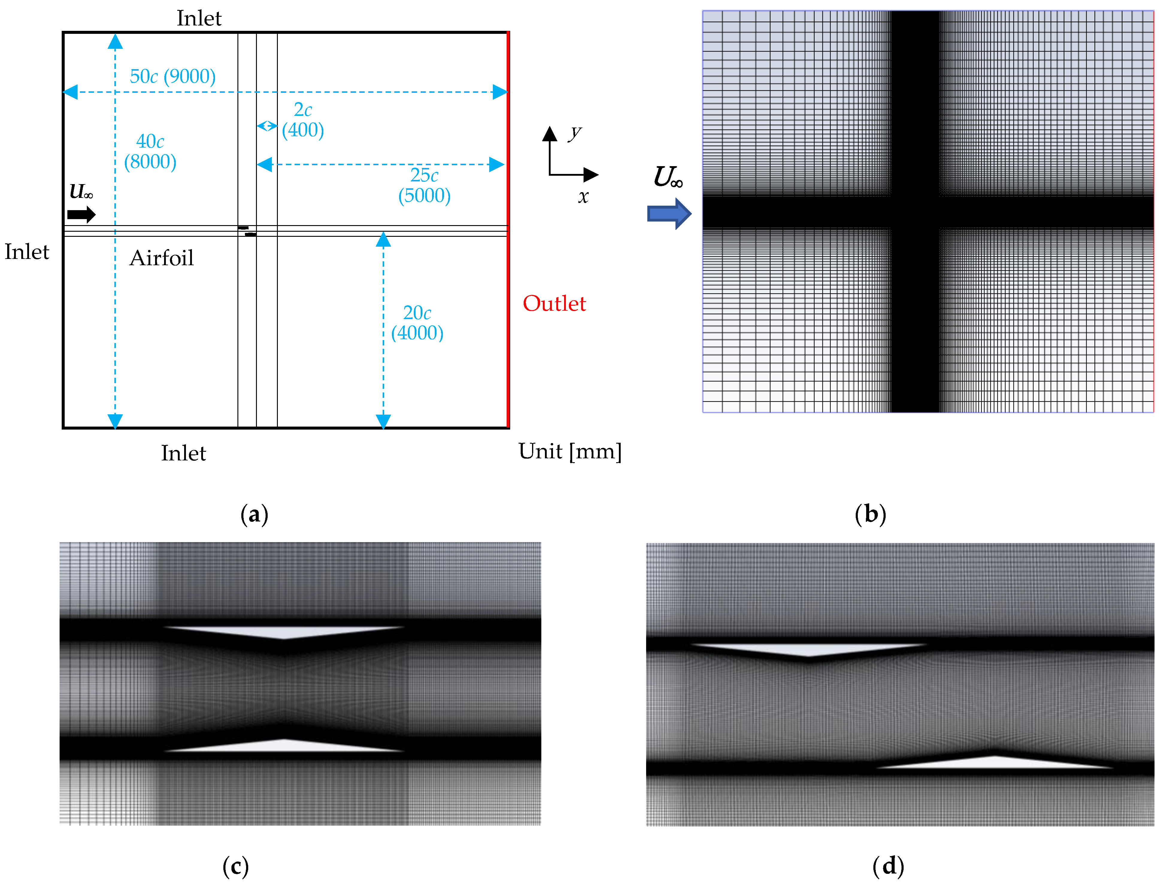
2.5. Numerical Simulation

Numerical simulations of two-dimensional incompressible steady flow were carried out and compared with the experimental results. The wing chord length was 200 mm. The computational mesh file was generated using ICEM software (ANSYS 2019 R3, Ansys Inc., Canonsburg, PA, USA). Figure 4 shows the computational domain and the grid distribution around the wing model. Four hundred grid points were set up on the wing surface, and the y+ value was adjusted to about 1. The boundaries of the computational domain were adjusted to more than 20 times the wing chord length. The Ansys Fluent solver was used with the RANS analysis. The Spalart–Allmaras (S-A) turbulence model was applied in the simulations, as previous biplane numerical studies [5,14,15]. In a previous study, the S-A model effectively estimated the flow with multi-wing configurations compared with other high-order modes [29,30]. Also, the numerical results with the k-ω SST turbulence model and mesh independence are discussed in Appendix A and Appendix B. The pressure-based solver with couple algorithm is applied. The convergence conditions of the residuals, velocity, and density were set to 10−6. The free-stream conditions were the same as the experimental conditions.
The further considerations of three-dimensional effects and the transition may need to fully predict the flow field, especially at high angles of attack. These may lead to discrepancies between the CFD predictions and the experimental data, especially in high-angle regimes near and beyond stall [31,32]. In previous studies, the transition effects can be neglected at small angles but show more influence near and beyond stall [32]. However, in the case of the Busemann biplane wing, unlike a single NACA 0012 wing, the flow turbulence between the wing elements is significant at high angles of attack. Moreover, the upper element has a flat upper surface, leading to significant separation even at a small angle of attack. So, the “fully turbulent” model may effectively predict the flow field even at the Reynold number range of this study.

3. Results and Discussions

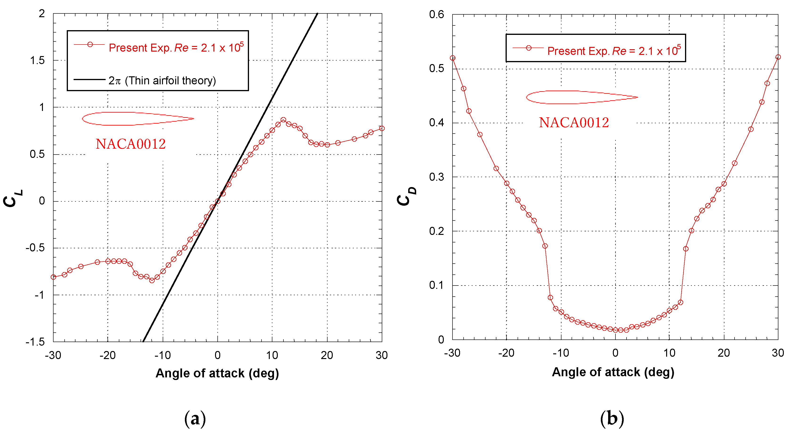
3.1. NACA0012 Airfoil Tests

First, the experiment with the single NACA0012 airfoil was carried out for evaluation of the two-dimensional results. Figure 5 shows the obtained results. The experimental conditions are the same as those for the biplane wing described in Section 2.2. Figure 5a,b show the drag coefficient and the lift coefficient, respectively. The experimental results show a good agreement with the reference data of the same rage of Reynolds number (Refs. [26,27]), indicating the feasibility of measuring the two-dimensional wing aerodynamic characteristics of this system.

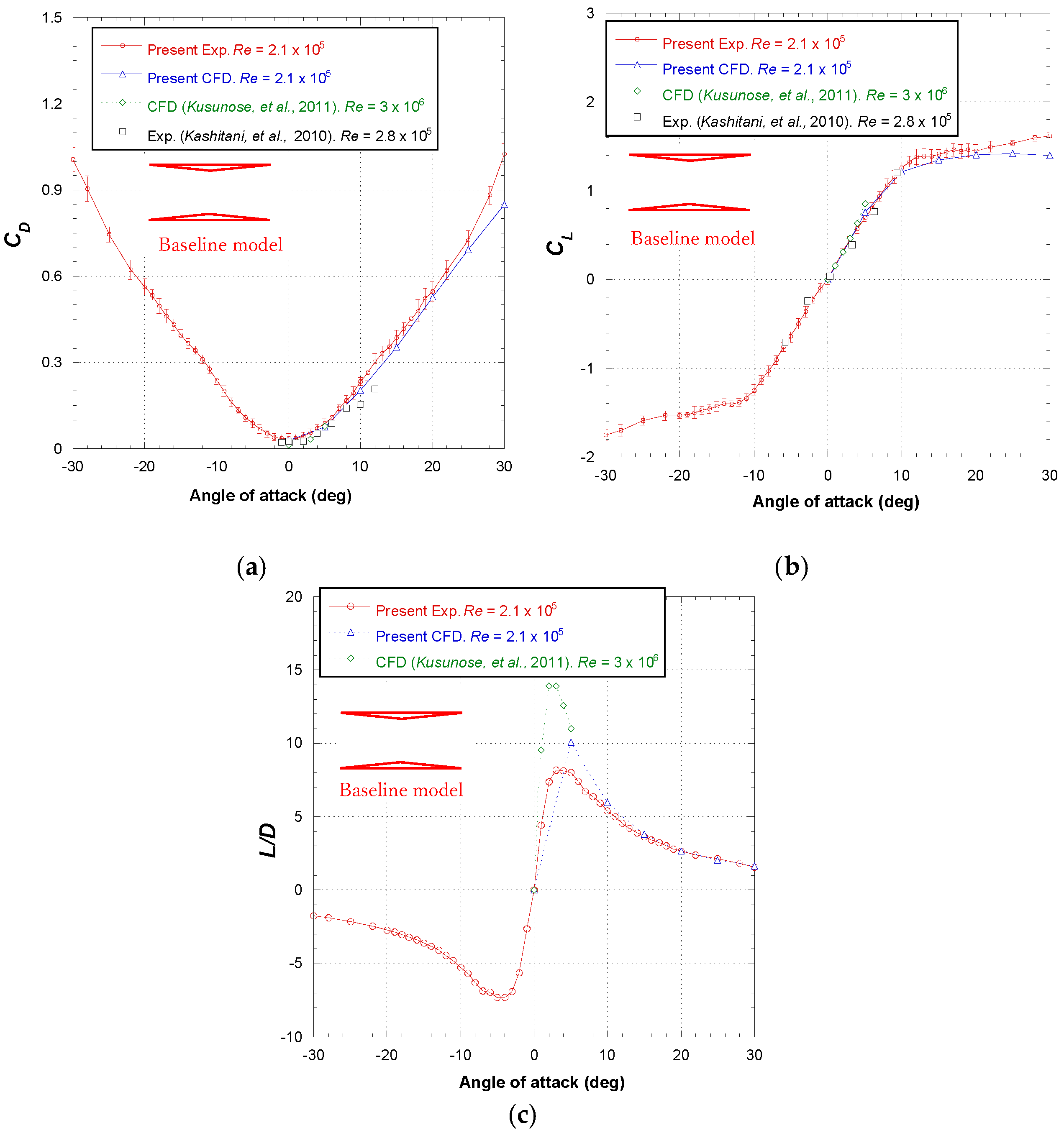
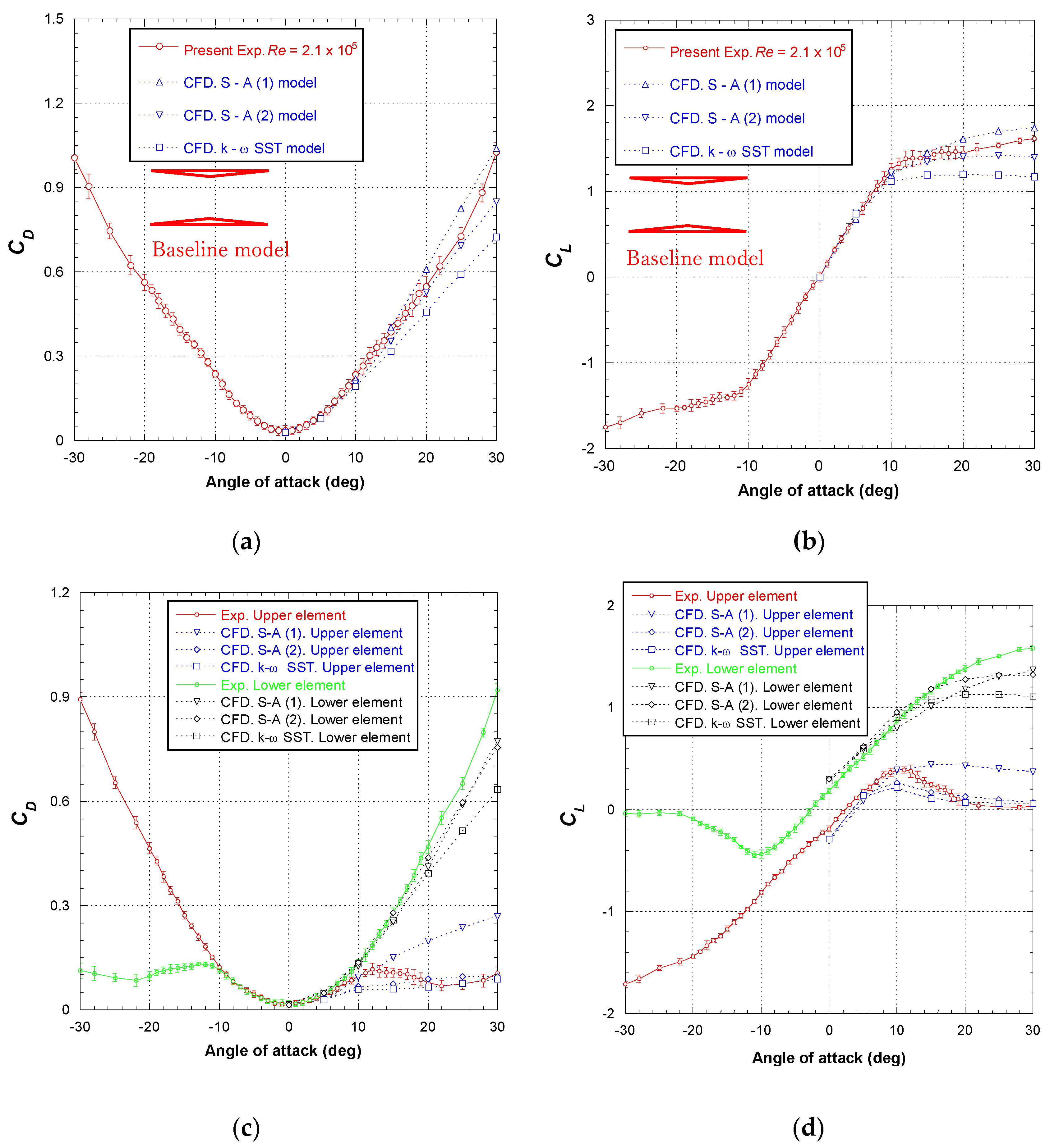
3.2. Baseline Model Test

Figure 6 shows the aerodynamic characteristics of the two-dimensional baseline model. The results for the biplane configuration are the sum of the upper and lower elements, as described by Equations (1) and (2). The standard deviation is also summarized from the results of the upper and lower elements. In the range of ±10 deg, the uncertainties of the lift and drag coefficients are about 0.04 and 0.014, respectively. When the angle of attack increases, the uncertainties increase but do not exceed 5% of the total lift and drag coefficients.
In Figure 6a, the drag coefficient is minimum at an attack angle of 0 deg and increases as the angle increases. The drag coefficients are almost constant between ±2 deg and increase rapidly from 5 to 30 deg. The results show a good agreement with Ref. [17] in the range from 0 to 8 deg, but the difference becomes larger when the angle of attack increases above 10 deg. In Ref. [17] (Kashitani, et al., 2010), the drag was calculated from the velocity deficit in the wake of the model, which has difficulty estimating the drag at a high angle of attack due to a larger flow separation and unsteadiness in the flow. The experimental results are in good agreement with the results of CFD and Refs. [5,16] (Kusunose, et al., 2011).
Figure 6b shows the lift coefficient of the baseline model. As the baseline model can be regarded as an asymmetrical wing, the zero-lift angle is 0 deg. The lift coefficient increases as the angle of attack increases. The experimental results are agreed with the results of CFD and Refs. [5,6,17] in the range of 0 to 10 deg. For the angles above 20 deg, the CFD results show smaller values than the experimental results. The detailed results will be discussed from the following results of the upper and lower elements in the baseline configuration. Table 2 shows the lift slopes in the attack angle range of ±10 deg. The lift slopes are 0.129, 0.122, 0.127, and 0.124 in the experimental results, CFD simulations, and Refs. [16,17], respectively. Therefore, this experiment’s results show good accuracy compared with previous studies of the Busemann biplane. Also, the experimental results show good agreement with the lift coefficient estimated by the smoke line pattern method used in Ref. [17].
Figure 6c shows the lift-to-drag ratio data. In experimental results, the maximum value is 8.2 at 3 deg. For angles of attack above 3 deg, the lift-to-drag ratio decreases as the angle of attack increases. The CFD shows a larger value compared with experimental results at 5 deg. For angles of attack above 10 deg, the experimental results show good agreement with the numerical results and Ref. [16].
Figure 7 shows the aerodynamic characteristics of the upper and lower elements for the single configuration and baseline configuration. Figure 7a shows the drag coefficient results. For the single configuration, the minimum drag appears at 1 deg for the upper element and −1 deg for the lower element because of the difference of the inverted camber of the elements. When the angle of attack increases, the drag coefficient increases. The results of single elements show a bucket-shaped distribution, similar to the drag coefficient of laminar flow over an airfoil [33]. This is due to the shapes of the elements with the camber and their thinness (5% of the chord length). For the baseline model, the results show no significant difference with the case of the single wing in the range of ±5 deg. The drag coefficient of the upper element is lower than the results for the single wing at angles of attack above 5 deg. The reason is that the lower element’s presence changes the upstream flow to the upper element. Then, the effective angle of attack for the upper element is reduced due to the effects of the flow interference between the wing elements. The drag coefficient of the upper element increases up to 12 deg and decreases in the ranges from 12 to 22 deg. In contrast, the result for the lower element is larger than that for the single wing when the angle of attack increases. The experimental results are in good agreement with CFD results for the angle of attack smaller than 20 deg.
The lift coefficient results are shown in Figure 7b. For the single wing, the lift increases as the angle of attack increases. Stall appears at 11 deg for the single upper element and 12 deg for the single lower element. As the elements are thin, the lift slopes of both single elements are almost the same, at 0.086 for the upper element and 0.088 for the lower element. The upper element in the biplane configuration also stalled at 11 deg as the single upper element. The lift of the upper element decreases as the angle of attack increases and is almost constant for the angle above 20 deg. On the other hand, the lift coefficients of the lower element for the baseline model are lower than those for the single lower element in the range of 0 to 12 deg. For the angle above 12 deg, the lift coefficient becomes larger than those of the single lower element due to the accelerated flow between the biplane elements delaying the flow separation from the lower element. The lift of the baseline model is mainly generated from the lower element at high angles of attack, as found in previous studies [16,17,18]. The CFD results show smaller values than the experimental results for the angles above 20 deg. Other results for biplane configuration and single upper and lower elements are discussed in Appendix C.

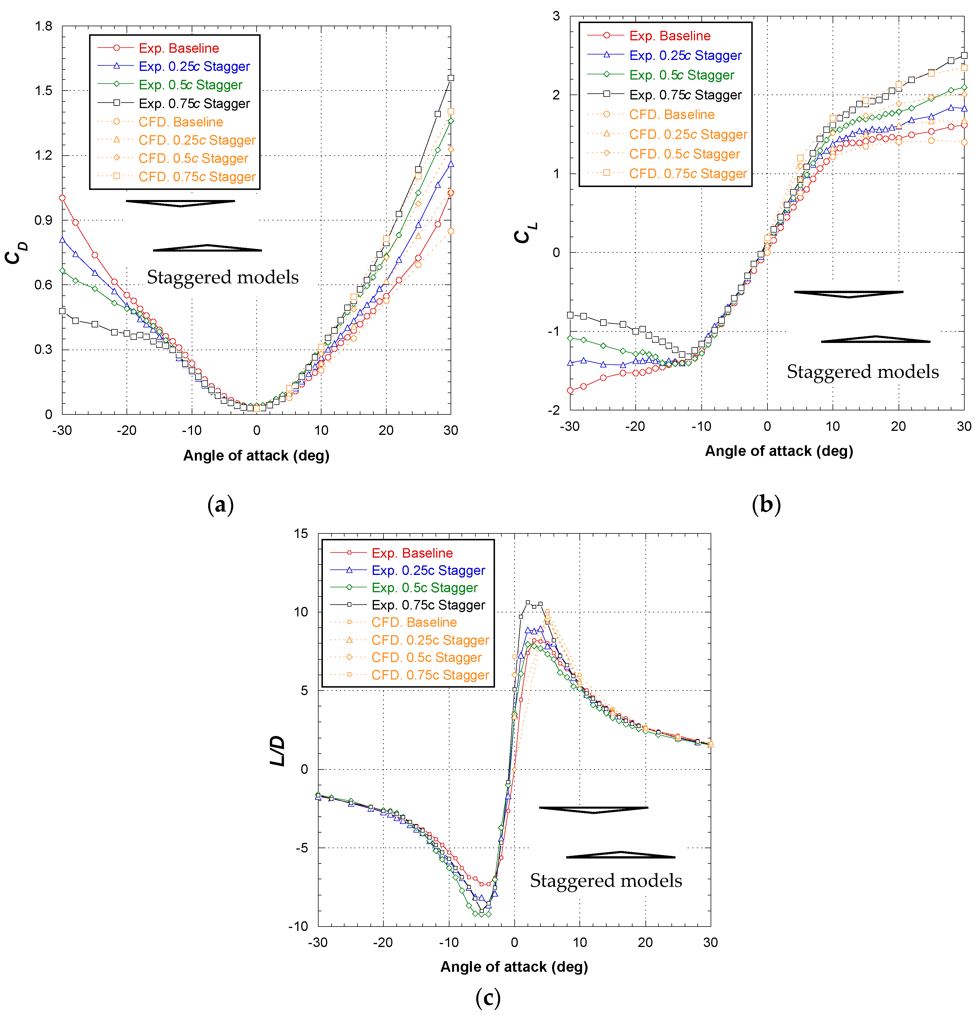
3.3. Stagger Effects

3.3.1. Drag and Lift Coefficient

Figure 8 shows the effect of different staggers on the total aerodynamic coefficient of the Busemann biplane.
Figure 8a shows the results for the total drag coefficient. The drag coefficient decreases as the stagger value increases at negative angles of attack, and it is clearly increased below an attack angle of −15 deg. From −2 to 3 deg, the staggered model results do not differ significantly from the baseline results. The increment due to the stagger becomes larger at high angles of attack. The reason for the increased drag is that the stagger changes the flow interference between the wing elements. Specifically, at high angles of attack, the drag coefficient of the upper element in the staggered model is larger than that of the baseline model. This is the main reason for the total drag increase. The experimental results show the same trend found with quantitative CFD simulations.
Figure 8b shows the results for the total lift coefficient. The stagger effect does not decrease the lift, even at negative angles of attack. The stagger effect clearly increases the lift coefficient at angles below −10 deg. From −10 to −3 deg, the total lift of the staggered model is not significantly different from the results of the baseline model. Table 3 shows the lift slopes of the staggered models. In the range of ±10 deg, the lift slopes are 0.129, 0.134, 0.144, and 0.147 for the baseline model, the 0.25c stagger model, the 0.50c stagger model, and the 0.75c stagger model, respectively. The lift increment due to the stagger effect is larger at attack angles above 10 deg. Also, wing stall does not appear in the staggered models until 30 deg. Although there are differences at high angles of attack, the experimental results show relative agreement with the trends of the CFD results. For the CFD results, the lift slopes are 0.122, 0.124, 0.135, and 0.152 for the baseline model, the 0.25c stagger model, the 0.50c stagger model, and the 0.75c stagger model, respectively. These values represent good agreement with the experimental results. Further, the results clarify that the Busemann biplane, which has upper and lower elements with different shapes, shows the same trend of an increased lift coefficient with the staggered configuration as the general biplane [18,25].
Figure 8c shows the lift-to-drag ratio data. The 0.25c stagger and 0.75c stagger models show larger values than the baseline models from 0 to 10 deg. On the other hand, the values obtained by using the 0.5c stagger model are smaller than those obtained from the baseline model. For the angles above 10 deg, there is no significant difference in lift-to-drag ratios for all models. The largest lift-to-drag is 10.5, which is confirmed at 3 deg for the 0.75c stagger model.

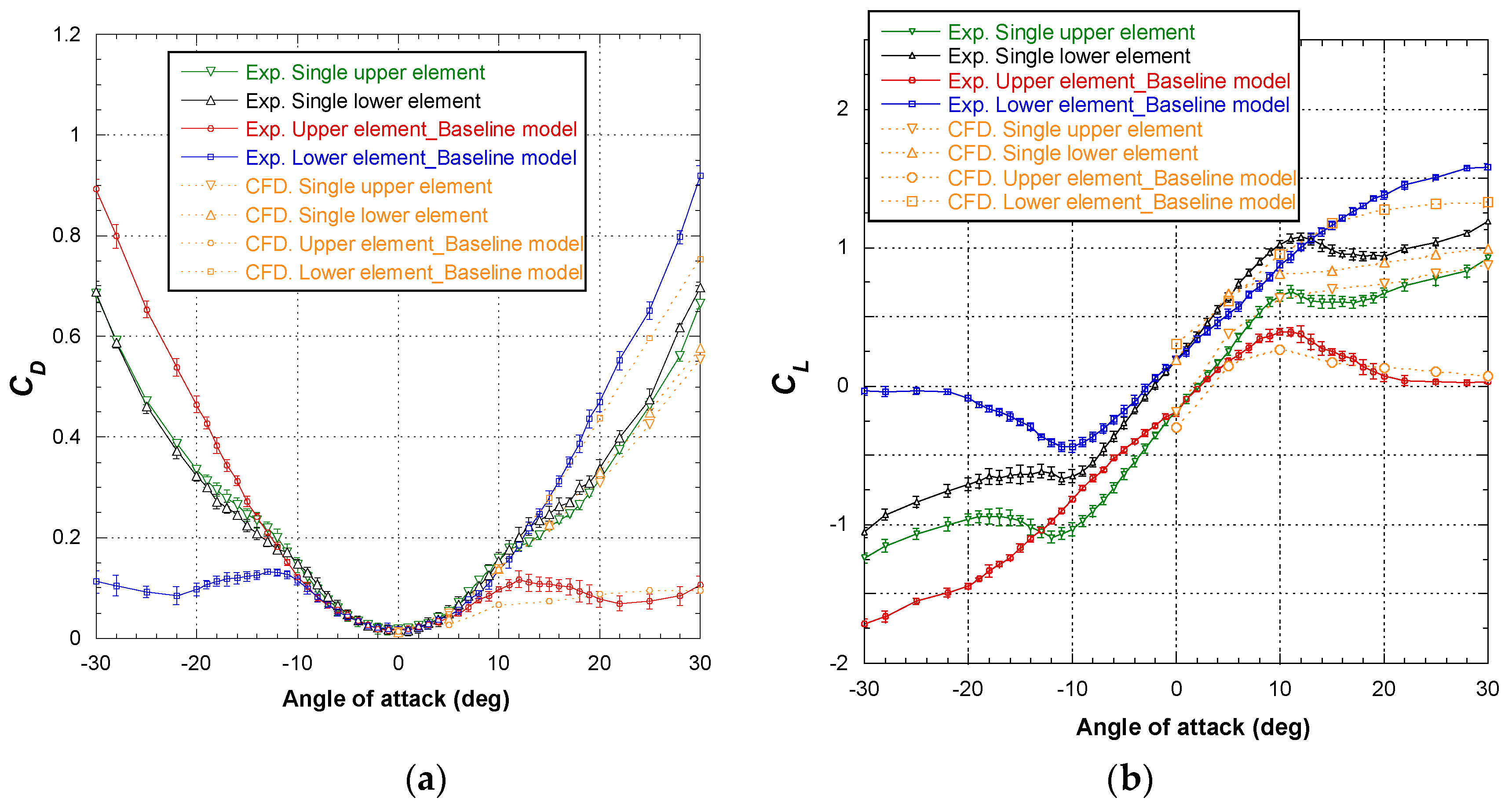
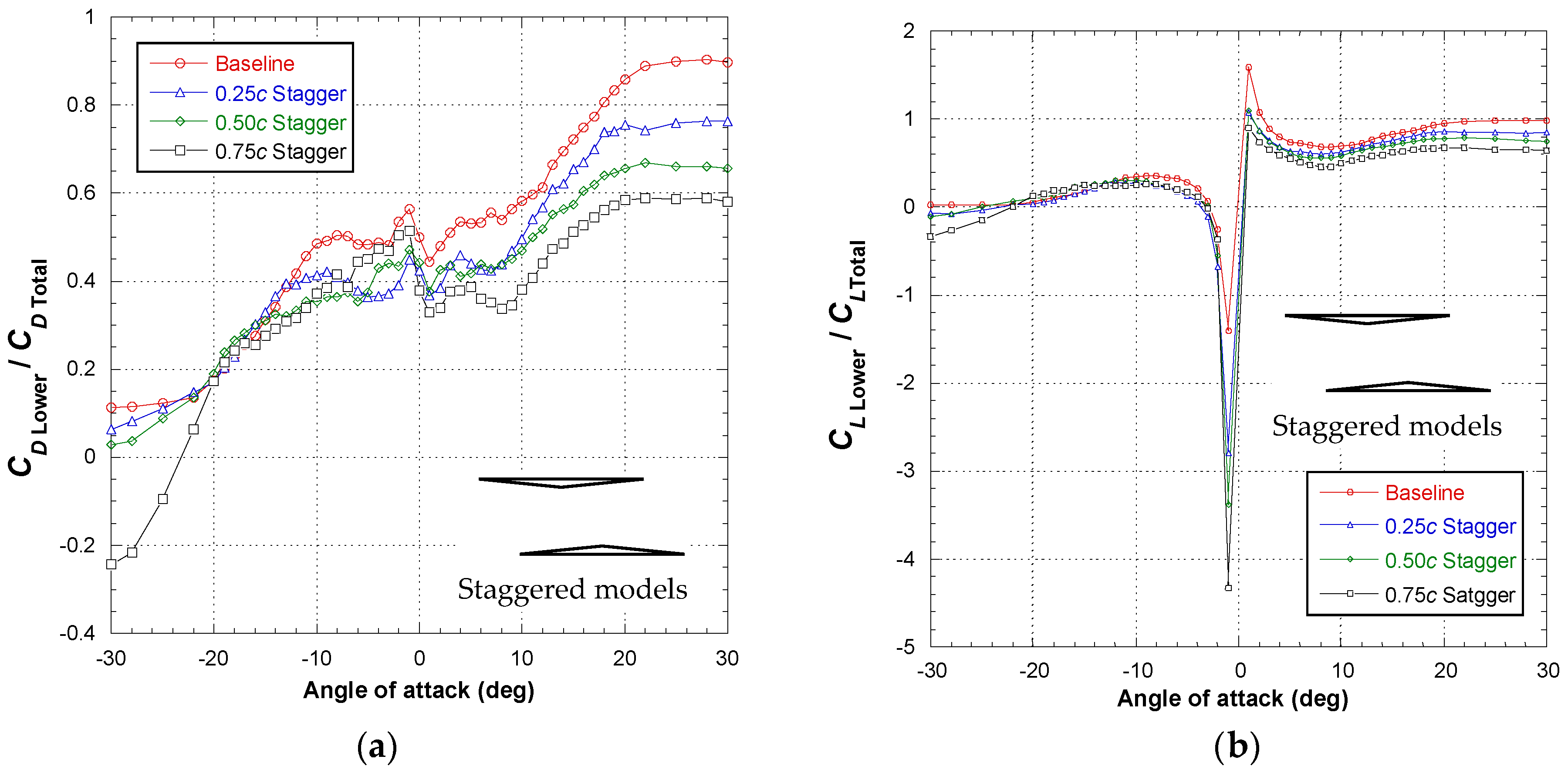
3.3.2. Contribution of the Lower Element to Total Performances of the Biplane

The results in Section 3.2 show that the lower element has an important role in overall performance of the biplane at high angles of attack. Therefore, in this section, the roles of the lower element as a ratio of the total results of the biplane configuration are discussed. Figure 9 shows the ratio of the aerodynamic forces of the lower element to the total forces of the biplanes.
Figure 9a shows the ratio for the drag coefficient. In the case of the baseline model, the ratio increases when the angle of attack increases. In the range from −30 to −22 deg, the drag of the lower element is about 0.1 of the total drag. From −10 to 5 deg, the ratio differs about 0.45 to 0.55, which means that the upper and lower elements produce nearly the same share of the total drag. Above 20 deg, the ratio is mostly constant, remaining about 0.88. In the staggered model, the ratio of the lower element to the total drag decreases as the stagger value increases for angles of attack above 0 deg. The results of the staggered model also clearly show the same trend as those of the baseline model. Above 20 deg, the ratios of all cases are mostly constant, precisely about 0.88, 0.75, 0.65, and 0.58 for the baseline model, the 0.25c stagger model, the 0.50c stagger model, and the 0.75c stagger model, respectively. Interestingly, the 0.75c stagger model shows a negative ratio below −25 deg. In this case, the drag of the lower element is negative, and the total drag coefficient is about 0.4, as shown in Figure 8a. It is considered that the lower element is pulled forward by the significant flow interference from the wake of the upper element.
Figure 9b shows the ratio for the lift coefficient of the lower element to the total lift of the biplanes. In the case of the baseline model, the ratio is almost 0 at angles of attack below −20 deg. When the angle of attack increases to −8 deg, the ratio also increases, up to 0.4. From −8 to −1 deg, the ratio decreases rapidly, and the lift ratio of the lower element is about −1.5 at −1 deg. The reason for this is that the biplane’s total lift approaches 0 at attack angles near 0 deg, as shown in Figure 6b. The ratio decreases at the range of angles from 1 to 8 deg because the lifts generated by both the lower and upper elements also increase. At this time, both the upper and lower elements of the baseline model generate positive lift, as shown in Figure 7b. Next, the ratio increases from 8 to 20 deg, and it is about 0.95 for angles of attack above 20 deg. This indicates that the lower element generates about 95% of the total lift at angles of attack above 20 deg. These results show a trend similar to that of a previous study on tandem wings [18], and quantitatively clarify the proportion of lift generated by the lower element in the Busemann biplane. In the staggered models, the ratio of the lower element to the total lift decreases as the stagger value increases at the angle above −10 deg. Above 20 deg, the ratios of all cases are mostly constant, precisely about 0.95, 0.85, 0.78, and 0.66 for the baseline model, the 0.25c stagger model, the 0.50c stagger model, and the 0.75c stagger model, respectively. However, the results of the staggered models show a negative value at angles of attack below −20 deg. In this case, the vortex generated from the leading edge of the upper element affects the flow field around the lower element, which causes the lower element to have a positive lift even at negative angles of attack. In this case, the total lift coefficients of the staggered models are negative at angles of attack below −25 deg, as shown in Figure 8b.

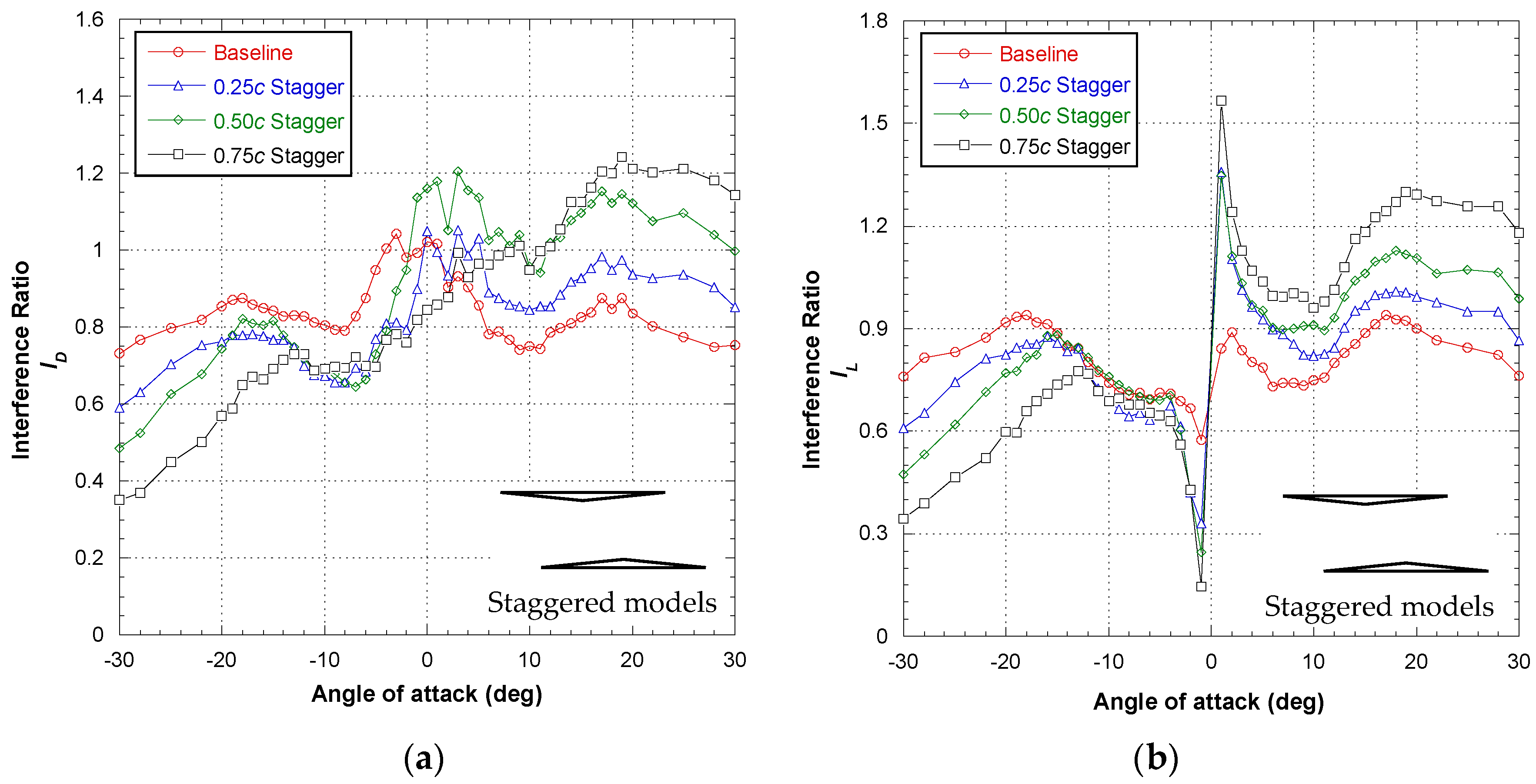
3.3.3. Interference Ratio

Figure 10 shows the interference ratios of the aerodynamic forces, which were calculated from the results of the biplane configuration and the biplane’s individual elements in the single configuration as follows:
I D = C d ( T o t a l ) C d ( S i n g l e _ U p p e r ) + C d ( S i n g l e _ L o w e r )
I L = C l ( T o t a l ) C l ( S i n g l e _ U p p e r ) + C l ( S i n g l e _ L o w e r )
where ID and IL are the drag and the lift interference ratios, respectively, and Cd(Single_Upper), Cd(Single_Lower), Cl(Single_Upper), and Cl(Single_Lower) are the respective drag and lift results for the single upper and lower elements, as shown in Figure 7. Note that Cd(Total) and Cl(Total) are defined by Equations (1) and (2) in Section 2.4.
Figure 10a shows the drag interference ratio calculated with Equation (3). For the baseline model results, the ratio is almost 1.0 near an angle of attack of 0 deg. As the angle of attack increases, the drag interference coefficient becomes less than 1, and the total drag of the biplane is less than the sum of the single upper and lower elements because of flow interference. In the staggered models, the same trend is observed for the 0.25c and 0.50c stagger models. However, the ratio increases from 0 to 17 deg for the 0.75c stagger model, unlike the other cases. Above 10 deg, the drag interference ratio increases with increasing stagger. For the 0.50c and 0.75c stagger models, the drag interference ratio is greater than 1 above 13 deg.
Figure 10b shows the results of the lift interference ratio calculated with Equation (4). For the baseline model, the lift interference ratios are less than 0.95 at all angles of attack, which shows that the total lift of the biplane is less than the sum of the single upper and lower elements. For angles of attack above 0 deg, the change in the lift interference ratio shows the same trend as the results of the drag interference ratio in Figure 10a. The maximum value of the interference ratio is about 0.94 at an attack angle of 17 deg. The results of the staggered model show a trend similar to that of the baseline model. From 0 deg, the lift interference ratio increases as the stagger value increases. However, the lift interference ratio decreases as the stagger value increases at attack angles below 0 deg.

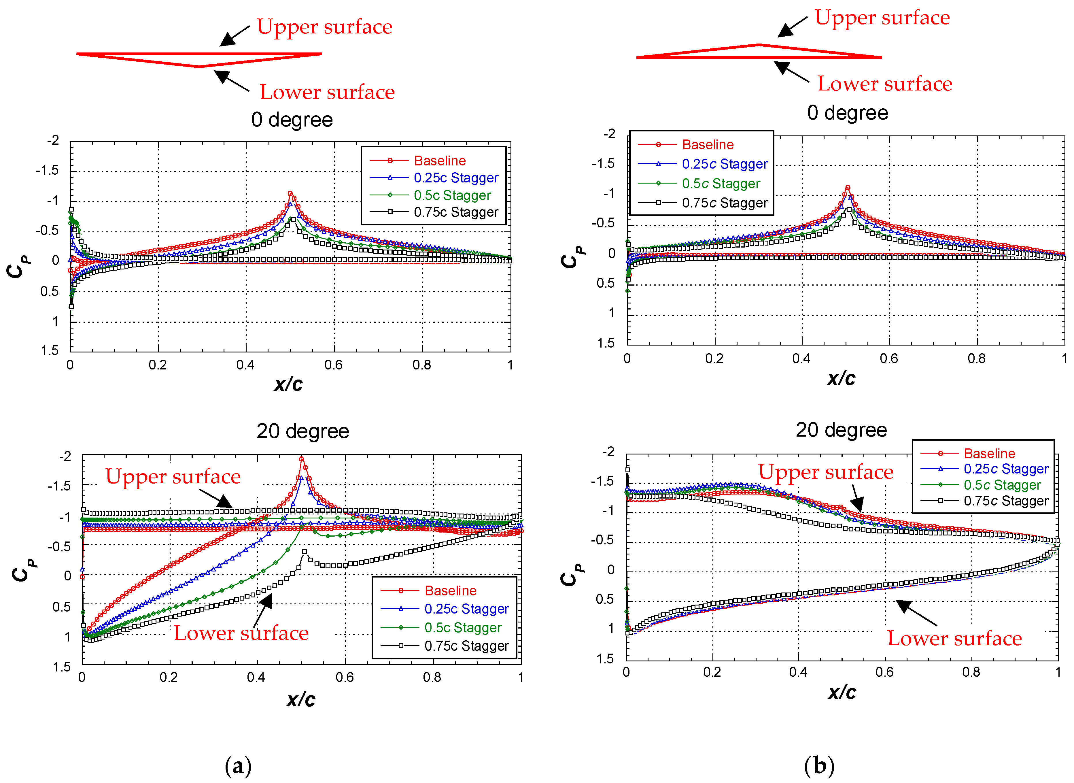
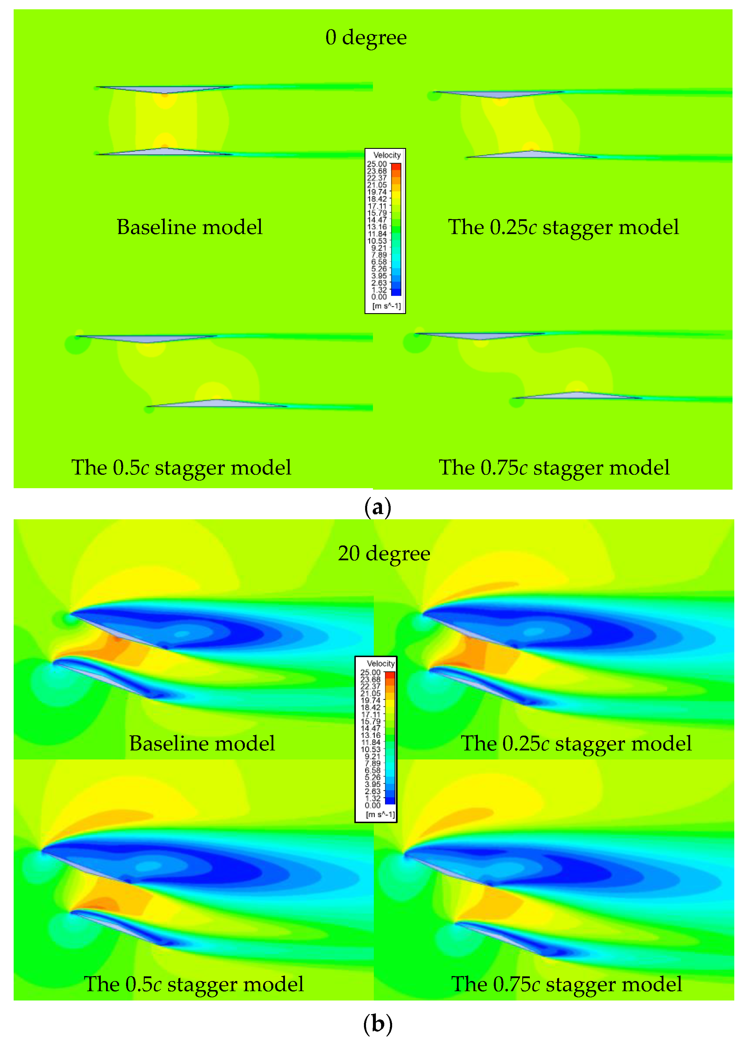
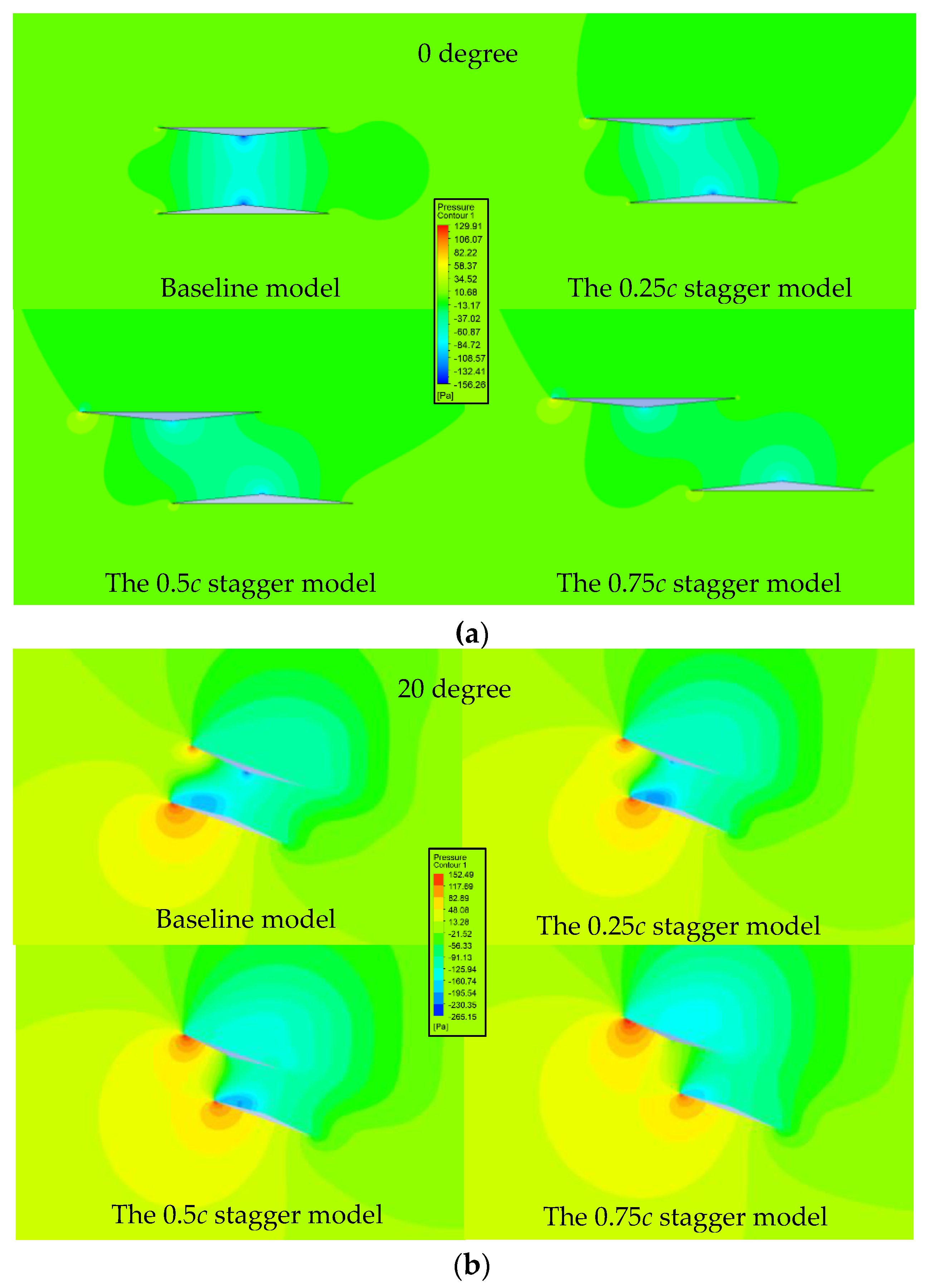
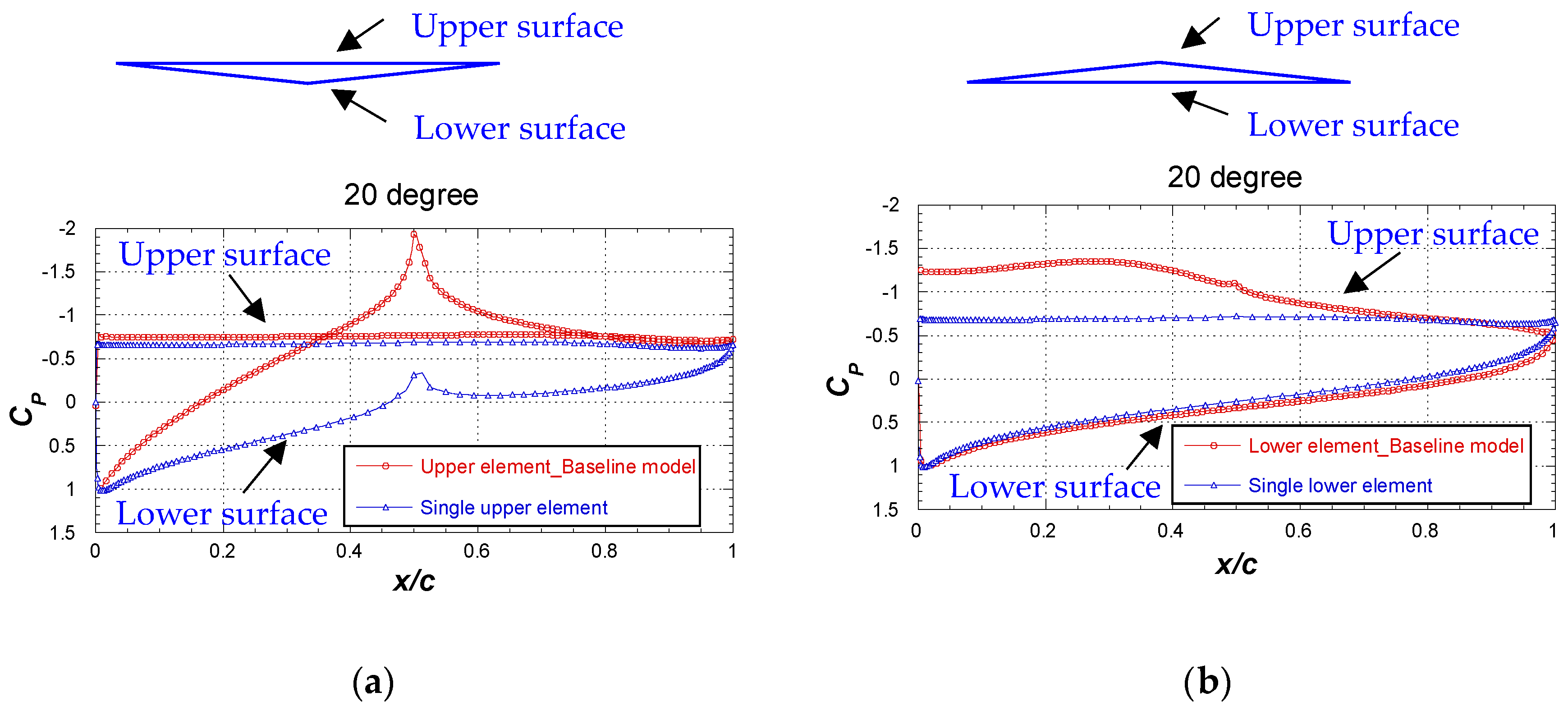
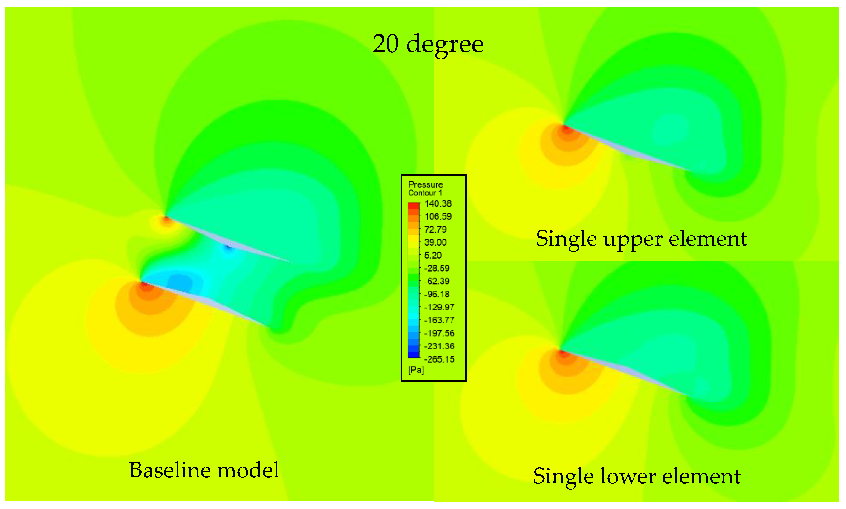
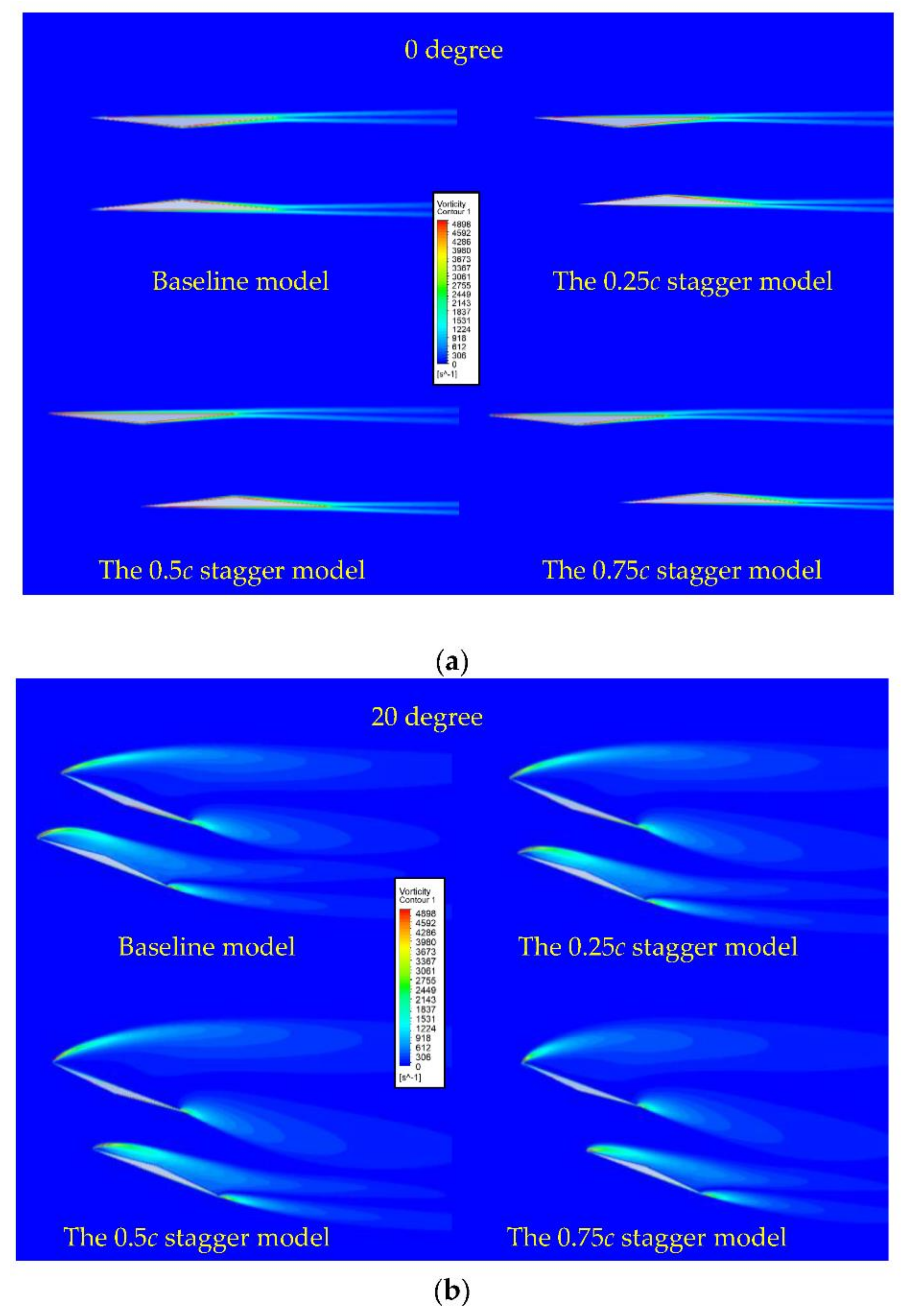
3.3.4. Pressure and Velocity Distribution around the Models

Figure 11 shows the pressure coefficient on the airfoil surface of the staggered models.
The angles of attack are 0 deg and 20 deg, respectively. The stagger effects increase the pressure coefficient on the lower surface of the upper element. At 20 deg, the effects are more significant. The results indicate that the upper elements generated more lift and drag when the stagger value increased. In Figure 11b, the pressure coefficient on the lower surface shows nearly the same in all cases for the lower element. At 0 deg, the peak value of the pressure coefficient at the wing center increases when the stagger value increases. At 20 deg, the stagger slightly changes the pressure coefficient on the upper surface from 0.2c to 0.6c position. Therefore, the increment of lift and drag generated by the upper element leads to the increment of the total lift and drag of the biplane model when the stagger value increases, as shown in Figure 8.
Figure 12 shows the CFD results of the velocity distribution around the models. The angles of attack are 0 deg and 20 deg, respectively.
At 0 deg, the flow is accelerated between the elements of the baseline model. At 20 deg, a significant separation and longitude vortex occur belong the upper surface of all cases. Due to the effects of accelerated flow between the biplane elements, the separation along the upper surface of the lower element is delayed. In Figure 12b, the separated flow from the lower wing’s leading edge is pressed more strongly to the wing surface when the stagger value is increased. This indicates the stagger effect of the leading-edge separation of the lower element in a biplane configuration. The vorticity distribution is discussed in Appendix D.
Figure 13 shows the pressure distribution around the models. At 0 deg, the baseline model shows the symmetric pressure distribution. When the stagger value increases, the high-pressure area near the leading edge of the upper element becomes more extensive. At 20 deg, the baseline configuration shows a sizeable high-pressure area near the lower surface of the lower element. Also, the high-pressure area below the upper element is smaller than that of the lower element. The results show that the lower element of the biplane generates more lift than the upper element. Compared with the baseline model, the high-pressure positioned near the leading edge of the upper element becomes more extensive in the staggered models. As the stagger value increases, the size of the high-pressure area also increases. Therefore, the lift generated by the upper element increases when the stagger value increases.

4. Conclusions

In this study, the low-speed performances of the Busemann biplane and the effect of stagger were investigated by wind tunnel tests and CFD simulations. The relative contributions of the lower and upper elements to total aerodynamic characteristics of the biplane were also clarified.
The lower element generated most of the lift and drag of the Busemann biplane (or the baseline biplane model with no stagger) at high angles of attack. At angles above 20 deg, the contribution of the lower element to total aerodynamic characteristics is almost constant, with 95% of the total lift and 88% of the total drag. The total lift and drag of the baseline model were smaller than the sum of the individual elements that were treated as a single configuration.
The increments of lift and drag due to the stagger effects were confirmed, especially at high angles of attack. When the stagger value increases, the high-pressure area near the leading edge of the lower surface of the upper element also increases, which increases the lift and drag of the upper element. This is the main reason for the increments of total lift and drag of the biplane model. On the other hand, the contribution of the lower element to total lift decreased as the stagger value increased. The stagger effects also prevented the leading-edge separation of the lower element in the biplane configuration and increased the lift slopes of the biplane model.
The CFD simulations showed good agreement with the experimental results.

Author Contributions

Conceptualization, T.D.N.; methodology, T.D.N.; software, ICED and Ansys Fluent; validation, T.D.N.; formal analysis, T.D.N. and M.K.; investigation, T.D.N., M.K. and M.T.; writing—original draft preparation, T.D.N.; writing—review and editing, T.D.N., M.K., M.T. and K.K. All authors have read and agreed to the published version of the manuscript.

Funding

This research received no external funding.

Institutional Review Board Statement

Not applicable.

Informed Consent Statement

Not applicable.

Data Availability Statement

Data are contained within the article.

Acknowledgments

The authors would like to thank K. Tsuji and M. Sugano, National Defense Academy, for their assistance during the wind tunnel experiments.

Conflicts of Interest

The authors declare no conflict of interest.

Nomenclature

cairfoil chord length, mm
Cllift coefficient
Cddrag coefficient
ILlift interference ratio
IDdrag interference ratio
hheight of test section, mm
twing thickness, mm
Ufreestream velocity
Gspacing between wing elements, mm
Subscripts
UpperThe upper element (wing)
LowerThe lower element (wing)
SingleThe single configuration (individual wing)
BiplaneThe biplane configuration

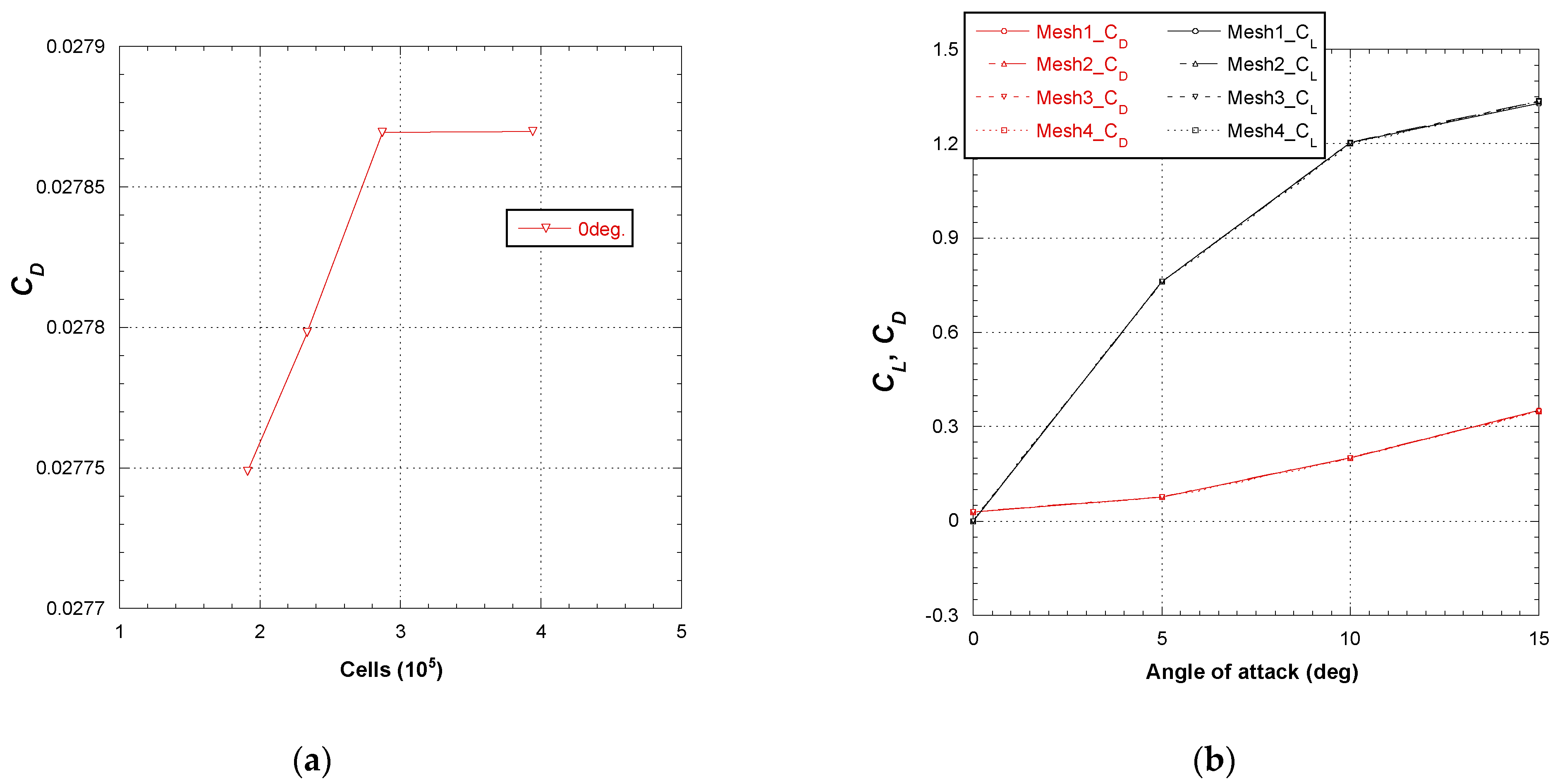
Appendix A. Grid Independence for Numerical Simulations

The grid independence of simulation results is investigated. The overview for grid generation is discussed in Section 2.5. Table A1 shows the grid settings for the grid independence investigation. Four different sets of grids are used. The y+ value of the grid is approximately 1, which means that the height of the first grid element nearest the airfoil is approximately 2 × 10⁻⁵ m. Simulations were performed using the software ANSYS 2019 R3. The results are shown in Figure A1. In Figure A1a, the drag coefficient convergence when the grid point between the upper and lower elements increases to 300 points. Figure A1b shows the lift-and-drag coefficient results when using four sets of grids. The results show no significant difference in the results of four grid sets. For the above considerations, Mesh 3 with 300 points between the wing elements is chosen for this study’s numerical simulations.
Table A1. The detail of mesh generation for the baseline model.
Mesh 1Mesh 2Mesh 3Mesh 4
Grid point on the element surface400400400400
Grid point between the wing elements120200300500
Total cells190,995233,795287,295394,295
Figure A1. Grid independence of numerical simulation for baseline model: (a) grid convergence at 0 degrees; (b) lift-and-drag ratio of 4 mesh systems.
Aerospace 09 00197 g0a1

Appendix B

The effects of turbulence models for the numerical simulations are investigated. The FLUENT codes are used in the simulations. Table A2 shows the setting parameters [34]. The Spalart-Allmaras (S-A) and the k-ω SST turbulent model, which validated for the wide flow ranges, were applied. The results of the baseline configuration are shown in Figure A2. Figure A2a,b show the total lift-and-drag coefficient results. From 0 to 10 deg, all three models show good agreement with experimental results. Above 10 deg, the S-A (1) and the S-A (2) models show values closer to the experimental results than the k-ω SST model. The detailed results of upper and lower elements are shown in Figure A2c,d. The S-A (1) and the S-A (2) models show larger values and are closer to the experimental results than the results of the k-ω SST model for the upper element at angles above 10 deg. However, the S-A (2) and k-ω SST models show smaller values than S-A (1) for the lower element at the angles above 10 deg, close to the experimental results. Following upper results, the S-A (2) setting is chosen to perform this study’s simulations.
Figure A2. Investigations of turbulence model in numerical simulations, baseline configuration: (a) total drag coefficient; (b) total lift coefficient; (c) drag coefficient of upper and lower elements; (d) lift coefficient of upper and lower elements.
Aerospace 09 00197 g0a2
Table A2. The simulation parameters.
ParametersS-A (1)S-A (2)k-ω SST
SolverDensity-based Pressure-basedPressure-based
Turbulence modelSpalart–AllmarasSpalart–Allmarask-ω SST
AlgorithmAUSMCoupleCouple
Spatial discretizationFlow: 1-orderPressure: 2-orderPressure: 2-order
Momentum: 2-order upwindMomentum: 2-order upwind
Modified Turbulent viscosity: 2-oder upwindModified turbulent viscosity: 1-order upwindTurbulent kinetic energy: 2-oder upwind
Specific dissipation rate: 2-order upwind

Appendix C

Figure A3 shows the CFD results of pressure coefficient on the airfoil surface of the wing elements as a single configuration and the biplane configuration. The angle of attack is 20 deg. In comparison with the single configuration, the pressure coefficients on the lower surface of the upper element and the upper surface of the lower element decrease in a biplane configuration. Figure A4 shows the pressure distribution results at 20 deg. The single upper element and the single lower element show qualitatively similar trends because the elements are considered thin, with the thickness being small (5%). The biplane configuration shows a sizeable high-pressure area near the lower surface of the lower element. Also, the high-pressure area below the upper element is smaller than that of the lower element. Therefore, it is clear that the lower element of the biplane generates more lift than the upper element.
Figure A3. Comparison of pressure coefficient in airfoil surface of the wing elements as single configuration and baseline configuration (CFD results): (a) upper element; (b) lower element.
Aerospace 09 00197 g0a3
Figure A4. Pressure distributions around the wing elements as single configuration and the baseline configuration (CFD results) at 20 degrees.
Aerospace 09 00197 g0a4

Appendix D

Figure A5 shows the CFD results of the vorticity distribution around the models. At 0 deg, the vorticity distributions without large flow separations have no significant difference in all cases. At 20 deg, strong vortices are generated at the leading and trailing edge of the upper and lower elements. The vortices generated by the leading-edge separation of the lower element is pushed to the vicinity of the lower element’s surface due to the effects of accelerated flow between the biplane elements.
Figure A5. Vorticity distributions around the staggered biplane configuration (CFD results): (a) 0 degrees; (b) 20 degrees.
Aerospace 09 00197 g0a5

References

  1. Low-Boom Flight Demonstration, NASA. Available online: https://www.nasa.gov/X59 (accessed on 15 September 2021).
  2. Silent Supersonic Transport Technologies, JAXA. Available online: https://www.aero.jaxa.jp/eng/research/frontier/sst/ (accessed on 15 September 2021).
  3. RUMBLE Projects, European Union’s Horizon. 2020. Available online: https://rumble-project.eu/i/ (accessed on 15 September 2021).
  4. Kusunose, K.; Matsushima, K.; Obayashi, S.; Furukawa, T.; Kuratani, N.; Goto, Y.; Maruyama, D.; Yamashita, H.; Yonezawa, M. Aerodynamic Design of Supersonic Biplane, Cutting Edge and Related Topics; The 21st century COE Program; International COE of Flow Dynamic Lecture Series; Tohoku University Press: Sendai, Janpan, 2007; Volume 5, pp. 1–239. [Google Scholar]
  5. Kusunose, K.; Matsushima, K.; Maruyama, D. Supersonic biplane–A review. In Progress in Aerospace Sciences; Elsevier: Amsterdam, The Netherlands, 2011; Volume 47, pp. 53–87. [Google Scholar]
  6. Kuratani, N.; Ogawa, T.; Yamashita, H.; Yonezawa, M.; Obayashi, S. Experimental and Computational Fluid Dynamic Around Supersonic Biplane for Sonic Boom Reduction. AIAA Paper 2007-3674. In Proceedings of the 28th AIAA Aeroacoustics Conference, Rome, Italy, 21–23 May 2007. [Google Scholar]
  7. Nagai, H.; Oyama, S.; Ogawa, T.; Kuratani, N.; Asai, K. Experimental Study on Interference Flow of a Supersonic Busemann Biplane using Pressure-Sensitive Paint Technique. ICAS-2008-3.7.5. In Proceedings of the 26th International Congress of the Aeronautical Sciences, Anchorage, AK, USA, 14–19 September 2008. [Google Scholar]
  8. Yamashita, H.; Kuratani, N.; Yonezawa, M.; Ogawa, T.; Nagai, H.; Asai, K.; Obayashi, S. Wind Tunnel Testing on Start/Unstart Characteristics of Finite Supersonic Biplane Wing. Int. J. Aerosp. Eng. 2013, 231434. [Google Scholar] [CrossRef]
  9. Maruyama, D.; Matsushima, K.; Kusunose, K.; Nakahashi, N. Three-Dimensional Aerodynamic Design of Low-Wave-Drag Supersonic Biplane Using Inverse Problem Method. J. Aircr. 2009, 46, 1906–1918. [Google Scholar] [CrossRef] [Green Version]
  10. Nguyen, T.D.; Kashitani, M.; Kusunose, K.; Taguchi, M.; Takita, Y. Analysis of a Wing–Fuselage Biplane with Trailing-Edge Flaps in Low-Speed Flow. J. Aircr. 2021, 59, 350–363. [Google Scholar]
  11. Kashitani, K.; Nguyen, T.D.; Taguchi, M.; Takita, Y.; Kusunose, K. Aerodynamic characteristics on Busemann Biplane by Wake Measurements in Low-speed Wind Tunnel. Trans. Jpn. Soc. Aeronaut. Space Sci. 2021, 64, 258–266. [Google Scholar] [CrossRef]
  12. Yamazaki, W.; Kusunose, K. Biplane-Wing /Twin-Body-Fuselage Configuration for Innovative Supersonic Transport. J. Aircr. 2014, 51, 1942–1952. [Google Scholar] [CrossRef]
  13. Yamashita, H.; Obayashi, S.; Kusunose, K. Reduction of Drag Penalty by means of Plain Flaps in the Boomless Busemann Biplane. Int. J. Emerg. Multidiscip. Fluid Sci. 2009, 1, 141–164. [Google Scholar]
  14. Patidar, V.K.; Yadav, R.; Joshi, S. Numerical investigation of the effect of stagger on the aerodynamic characteristics of a Busemann biplane. Aerosp. Sci. Technol. 2016, 55, 252–263. [Google Scholar] [CrossRef]
  15. Ma, B.; Wang, G.; Wu, J.; Ye, Z. Avoiding Choked Flow and Flow Hysteresis of Busemann Biplane by Stagger Approach. J. Aircr. 2020, 57, 440–455. [Google Scholar] [CrossRef]
  16. Kuratani, N.; Ozaki, S.; Obayashi, S.; Ogawa, T.; Matsuno, T.; Kawazoe, H. Experimental and Computational Studies of Low-Speed Aerodynamic Performance and Flow Characteristics around a Supersonic Biplane. Trans. Jpn. Soc. Aeronaut. Space Sci. 2009, 52, 89–97. [Google Scholar]
  17. Kashitani, M.; Yamaguchi, Y.; Kai, Y.; Hirata, K.; Kusunose, K. Study on Busemann Biplane Airfoil in Low-speed Smoke Wind Tunnel. Trans. Jpn. Soc. Aeronaut. Space Sci. 2010, 52, 213–219. [Google Scholar] [CrossRef] [Green Version]
  18. Jones, R.; Cleaver, D.J.; Gursul, I. Aerodynamics of biplane and tandem wings at low Reynolds numbers. Exp. Fluids 2015, 56, 124. [Google Scholar] [CrossRef]
  19. Mueller, T.J.; Burns, T.F. Experimental Studies of the Eppler 61 Airfoil at Low Reynold Numbers. AIAA Paper 82-0345. In Proceedings of the 20th Aerospace Sciences Meeting, Orlando, FL, USA, 11–14 January 1982. [Google Scholar]
  20. Nguyen, H.A.; Mizoguchi, M.; Itoh, H. Unsteady Aerodynamic Characteristics of NACA0012 Airfoil Undergoing Constant Pitch-Rate Motions at Low Reynolds Numbers. Jpn. Soc. Aeronaut. Space Sci. Aerosp. Technol. 2020, 19, 111–119. (In Japanese) [Google Scholar] [CrossRef]
  21. Rasuo, B. Scaling between Wind Tunnels–Results Accuracy in Two-Dimensional Testing. Trans. Jpn. Soc. Aeronaut. Space Sci. 2012, 55, 109–115. [Google Scholar] [CrossRef] [Green Version]
  22. Ocokoljic, G.; Damljanovic, D.; Vukovic, D.; Rasuo, B. Contemporary Frame of Measurement and Assessment of Wind-Tunnel Flow Quality in a Low-Speed Facility. FME Trans. 2018, 46, 429–442. [Google Scholar] [CrossRef]
  23. Barlow, J.B.; Rae, W.H.; Pope, A. Low-Speed Wind Tunnel Testing, 3rd ed.; A Wiley-Interscience Publication: New York, NY, USA, 1999; pp. 353–361. [Google Scholar]
  24. Traub, L.W. Theoretical and Experimental Investigation of Biplane Delta Wings. J. Aircr. 2001, 38, 536–546. [Google Scholar] [CrossRef]
  25. Moschetta, J.M.; Thipyopas, C. Aerodynamic Performance of a Biplane Micro Air Vehicle. J. Aircr. 2007, 44, 291–299. [Google Scholar] [CrossRef]
  26. Ohtake, T.; Nakae, Y.; Motohashi, T. Nonlinearity of the Aerodynamic Characteristics of NACA0012 Aerofoil at Low Reynold Numbers. Trans. Jpn. Soc. Aeronaut. Space Sci. 2007, 55, 439–445. (In Japanese) [Google Scholar]
  27. Sheldahl, R.E.; Klimas, P.C. Aerodynamic Characteristics of Seven Symmetrical Airfoil Sections through 180-Degree Angle of Attack for Use in Aerodynamic Analysis of Vertical Axis Wind Turbines; SAND-80-2114; Sandia National Laboratories: Albuquerque, NM, USA, 1981. [Google Scholar]
  28. Ladson, C.L. Effects of Independent Variation of Mach and Reynolds Number on the Low-Speed Aerodynamic Characteristics of NACA0012 Airfoil Section; NASA TM-4047; NASA Langley Research Center Hampton: Hampton, VA, USA, 1988. [Google Scholar]
  29. Spalart, P.R.; Rumsey, C.L. Effective inflow conditions for turbulence Models in Aerodynamics Calculations. AIAA J. 2007, 45, 2544–2553. [Google Scholar] [CrossRef]
  30. Cai, Y.; Liu, G.; Zhu, W.; Tu, Q.; Hong, G. Aerodynamic Interference Significance Analysis of Two-Dimensional Front Wing and Rear Wing Airfoils with Stagger and Gap Variations. J. Aerosp. Eng. 2019, 32, 04019098. [Google Scholar] [CrossRef]
  31. Nandi, T.N.; Brasseur, J.G. Prediction and Analysis of the Nonsteady Transition and Separation Processes on the Oscillating Wind Turbine Airfoil using the γ-Reθ Transition Model. AIAA Paper 2016-0520. In Proceedings of the AIAA SciTech, San Diego, CA, USA, 4–6 January 2016. [Google Scholar]
  32. Wang, R.; Xiao, Z. Transition effects on flow characteristics around a static two-dimensional airfoil. Phys. Fluids 2020, 32, 035113. [Google Scholar]
  33. Van Dam, C.P. Natural Laminar Flow Airfoil Design Considerations for Winglets on Low-Speed Airplane. NASA Contractor Report 3853; Vigyan Research Associate, Inc.: Colonial Heights, VA, USA, 1984. [Google Scholar]
  34. Yang, L.; Zhang, G. Analysis of Influence of Different Parameters on Numerical Simulation of NACA0012 Incompressible External Flow Field under High Reynolds Number. Appl. Sci. 2022, 12, 416. [Google Scholar] [CrossRef]
Figure 1. Overview of the low-speed wind tunnel: (a) top view; (b) side view.
Aerospace 09 00197 g001
Figure 2. Experimental setting in the test section.
Aerospace 09 00197 g002
Figure 3. Experimental models: (a) single upper element; (b) single lower element; (c) baseline model (Busemann biplane—no stagger); (d) staggered models (three stagger lengths).
Aerospace 09 00197 g003
Figure 4. Meshes used for numerical calculations: (a) computational domain; (b) overview of grid; (c) grid distribution around the baseline model; (d) grid distribution around the 0.75c stagger model.
Aerospace 09 00197 g004
Figure 5. Results of single NACA0012 for balance measurement: (a) drag coefficient; (b) lift coefficient.
Aerospace 09 00197 g005
Figure 6. Aerodynamic characteristics of the baseline model: (a) drag coefficient; (b) lift coefficient; (c) lift-to-drag ratio.
Aerospace 09 00197 g006
Figure 7. Comparison of aerodynamic characteristics of the wing elements as single configuration and baseline configuration: (a) drag coefficient; (b) lift coefficient.
Aerospace 09 00197 g007
Figure 8. Effect of stagger on aerodynamic characteristics: (a) drag coefficient; (b) lift coefficient; (c) lift-to-drag ratio.
Aerospace 09 00197 g008
Figure 9. Ratios of the lower wing to the biplane performances: (a) ratio for drag coefficient; (b) ratio for lift coefficient.
Aerospace 09 00197 g009
Figure 10. Interference ratios of the biplane aerodynamic forces: (a) drag interference ratio; (b) lift interference ratio.
Aerospace 09 00197 g010
Figure 11. Comparison of pressure coefficient in airfoil surface of the staggered biplane configuration (CFD results): (a) upper element; (b) lower element.
Aerospace 09 00197 g011
Figure 12. Velocity distributions around the staggered biplane configuration (CFD results): (a) 0 degrees; (b) 20 degrees.
Aerospace 09 00197 g012
Figure 13. Pressure distributions around the staggered biplane configuration (CFD results): (a) 0 degrees; (b) 20 degrees.
Aerospace 09 00197 g013
Table 1. Experimental conditions.
Parameters
Flow velocity15 m/s
Reynold number2.1 × 105
The angle of attack−30~30 deg.
Balance measurement20 s for a pattern
5 Hz sampling frequency
Single configurationNACA0012
The single upper element
The single lower element
Biplane configurationThe Baseline model (No stagger)
The 0.25c stagger model
The 0.50c stagger model
The 0.75c stagger model
Table 2. Lift slopes of the baseline model.
Exp.CFDRef. [16]Ref. [17]
Lift slopes (±10 deg.)0.1290.1220.1270.124
Table 3. Lift slopes of the staggered models (±10 deg).
Baseline Model0.25c Stagger Model0.5c Stagger Model0.75c Stagger Model
Exp.0.1290.1340.1440.147
CFD0.1220.1240.1350.152
Publisher’s Note: MDPI stays neutral with regard to jurisdictional claims in published maps and institutional affiliations.

