Research on the Identification of Pilots’ Fatigue Status Based on Functional Near-Infrared Spectroscopy

Abstract

Fatigue can lead to sluggish responses, misjudgments, flight illusions and other problems for pilots, which could easily bring about serious flight accidents. In this paper, a wearable functional near-infrared spectroscopy (fNIRS) device was used to record the changes of hemoglobin concentration of pilots during flight missions. The data was pre-processed, and 1080 valid samples were determined. Then, mean value, variance, standard deviation, kurtosis, skewness, coefficient of variation, peak value, and range of oxyhemoglobin (HbO₂) in each channel were extracted. These indexes were regarded as the input of a stacked denoising autoencoder (SDAE) and were used to train the identification model of pilots’ fatigue state. The identification model of pilots’ fatigue status was established. The identification accuracy of the SDAE model was 91.32%, which was 23.26% and 15.97% higher than that of linear discriminant analysis (LDA) models and support vector machines (SVM) models, respectively. Results show that the SDAE model established in our study has high identification accuracy, which can accurately identify different fatigue states of pilots. Identification of pilots’ fatigue status based on fNIRS has important practical significance for reducing flight accidents caused by pilot fatigue.

1. Introduction

In recent years, with the rapid developments of aircraft design, manufacturing and maintenance, the reliability and safety of aircraft have improved significantly. However, aviation accidents and incidents caused by pilot fatigue still occur. Pilots are often fatigued due to a lack of sleep, long flights, night flying, transmeridian flight, as well as cabin noise, vibrations, and air pressure changes [1]. When pilots are in a state of fatigue, problems such as slower reaction speed, misjudgment, decreased operational ability, and flight illusion may occur, which will seriously affect flight safety. Therefore, how to quickly and accurately identify the fatigue state of pilots has become a core scientific problem in the field of aviation safety that needs to be solved urgently. The identification of pilot fatigue status has important theoretical and practical significance for ensuring flight safety, realizing pilot fatigue risk control, and formulating flight-related regulations.

Scholars at home and abroad have adopted various methods to detect the fatigue status of pilots. Subjective evaluation [2,3,4], physiological parameters [5,6,7], behavior characteristics [8,9,10,11,12], and flight parameters [13,14] are included in these methods. Among them, the monitoring of pilot fatigue state was more successfully achieved by physiological parameters than other methods. When pilots are fatigued, their physiological functions such as cardiac function, neurological function, and respiratory function change accordingly. Therefore, the fatigue status can be reflected by physiological indicators such as electroencephalogram (EEG) signals [15], electrocardiogram (ECG) signals [16], electromyogram (EMG) signals [17,18], and blood oxygen levels [19,20].

Functional near-infrared spectroscopy (fNIRS) is an emerging brain functional imaging technology. It has the advantages of low consumption, easy operation, portability, less interference from controlling operations, real-time detection, excellent temporal resolution and better spatial localization ability, etc., fNIRS is now widely used to monitor the degree of brain activation. Some scholars have found that fNIRS can reflect the fatigue state of the brain to a certain extent [21]. Zhao Yue used functional near-infrared spectroscopy to detect the fatigue state of drivers and found that as driving time increased, the absolute concentration of oxyhemoglobin in the left region of the prefrontal lobe of the brain tended to increase. The change of deoxyhemoglobin concentration in this region could be used to measure the fatigue level of drivers [22]. Xu et al. used functional near-infrared spectroscopy to investigate the synergistic mechanisms of different brain regions of participants during driving tasks and mental calculation tasks. The results showed that mental fatigue has an adverse effect on cognitive function [23]. Li et al. randomly divided the participants into two groups (driving and non-driving) and found that compared with the non-driving group, the concentration of oxygenated hemoglobin in the frontal cortex of the driving group was relatively increased [24].

In recent years, domestic and foreign scholars have used various algorithms to classify fatigue status based on fNIRS data, such as linear discriminant analysis (LDA), fisher linear discriminant (FLD) analysis, and support vector machines (SVM). Khan et al. collected fNIRS signals of the drivers’ prefrontal lobe area through a simulation experiment, and an LDA model was utilized to classify the drivers’ sleepiness and alertness [25]. Nguyen et al. collected fNIRS data of drivers in the awake and drowsy states, and the mean values of HbO and Hb concentration changes were analyzed to classify fatigue states based on the FLD method [26]. Zhang et al. induced fatigue through character 2-back working memory tasks, collected fNIRS, ECG, and respiratory data of participants, and used SVMs to detect mental fatigue based on various data sources. It was found that the accuracy of mental fatigue detection based on fNIRS data was higher than that of ECG and respiratory [27].

FNIRS provides a technical basis for researchers to continuously detect pilots’ brain signals during flight. The continuous improvement of denoising and modeling methods provides a reliable theoretical basis for the interpretation of the pilot’s operational behavior at the “brain-machine” level.

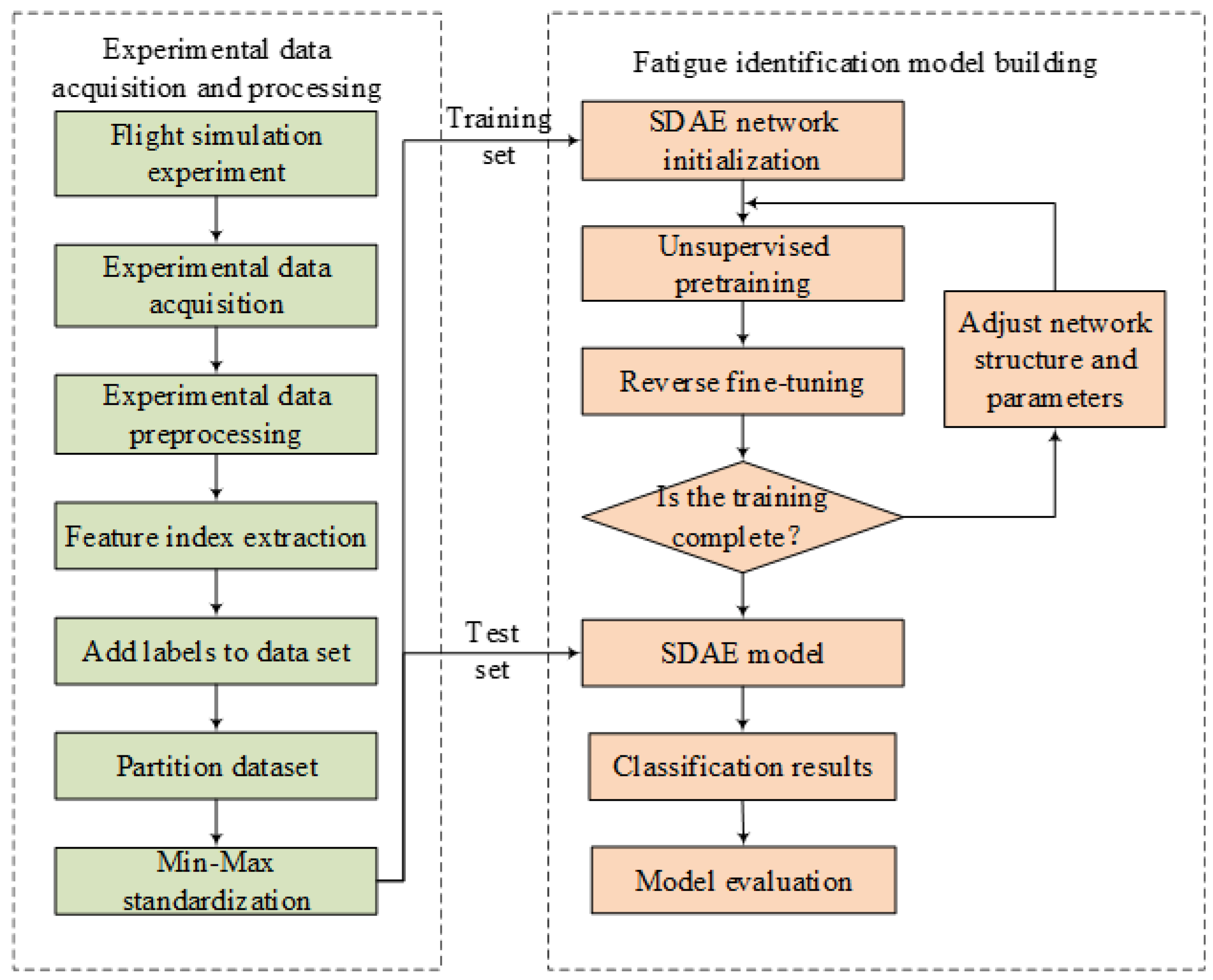
At present, there is little research on pilot fatigue based on fNIRS, with incomplete feature indicators and single identification methods. In this paper, the research on pilot fatigue state based on fNIRS is carried out to address the problems. The fatigue scale and fNIRS data were acquired on the basis of simulated flight experiments. Then the data were preprocessed to obtain the scale statistics and the relative HbO₂ concentrations for each channel. The characteristic indexes of the relative HbO₂ concentrations of each channel were extracted to establish the data set. The corresponding fatigue status labels were added to the data set. The data sets were min-max standardized, after which the data set was divided into training and test sets. Subsequently, the SDAE model was initialized. With the training set as the input, the network structure and parameters were adjusted through unsupervised pre-training and reverse fine-tuning steps. The test set was utilized to test the SDAE network model to obtain the classification results and evaluate the model. 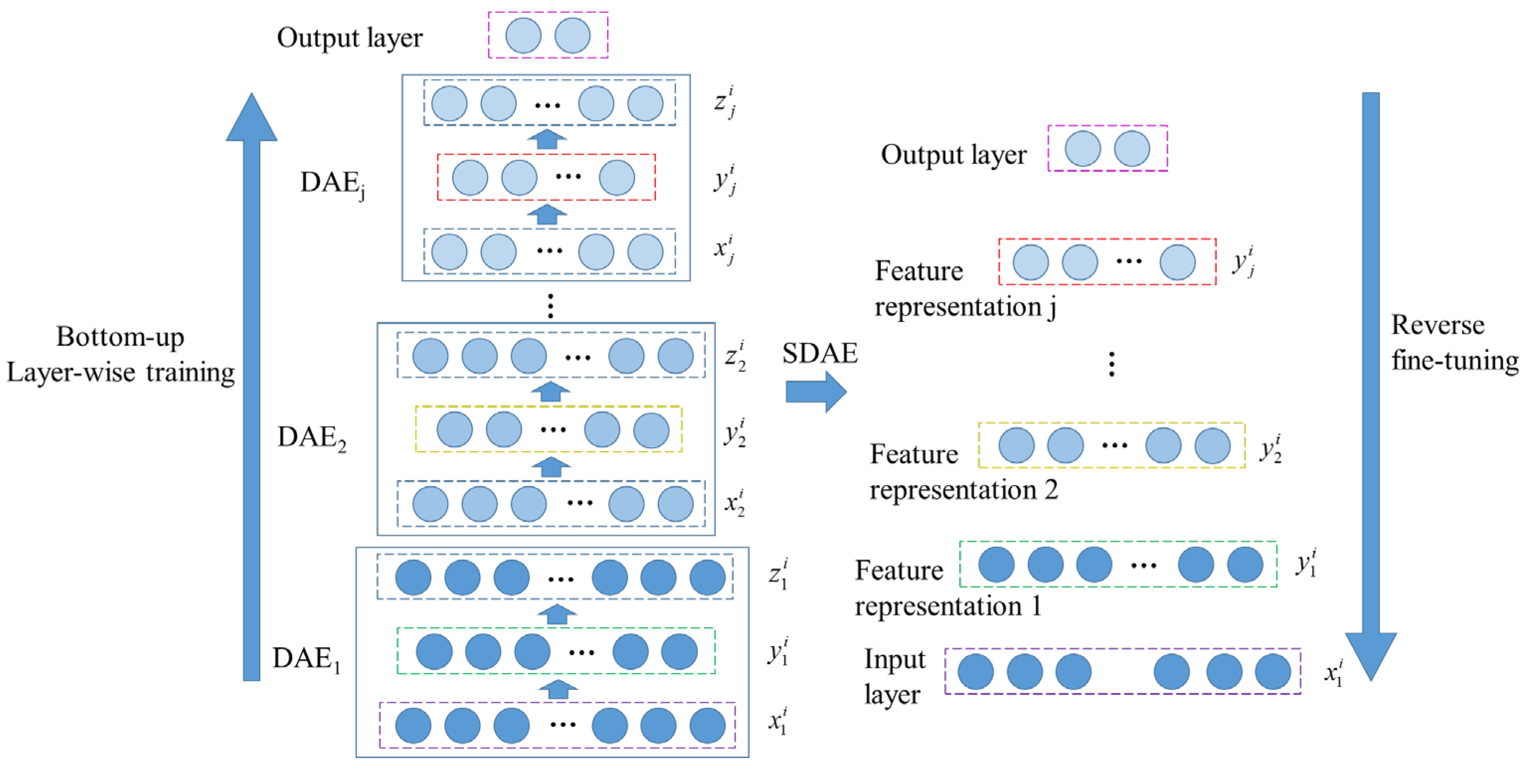Figure 1 shows the research framework.

The remainder of this paper is organized as follows: Details of the experimental content and research methodology are presented in Section 2. The results of the study are analyzed in Section 3. The discussion and future works are described in Section 4. We conclude the paper in Section 5.

2. Materials and Methods

2.1. Participants

Thirty pilots were recruited for the experiment, all of whom had obtained a Private Pilot License, Commercial Pilot License, and Instrument Rating License. The basic information is listed in

Table 1. Basic information of the participants.

Basic Information	Mean and Standard Deviation
Age	23.57 ± 1.42 (year)
Mean time of flight	291.25 ± 19.84 (h)

. The selected pilots were all right-handed, with normal or corrected vision, no history of serious medical conditions such as tumors, nephritis, or endocrine disorders and good sleep habits. Before the experiment, the participants were required to ensure sufficient sleep, avoid strenuous exercise, avoid smoking, drinking and other behaviors that excite or inhibit the central nervous system 24 h before the experiment and maintain a good mental state.

The experimental procedures were carried out in strict accordance with the Declaration of Helsinki. All experimenters received full instructions on the experimental procedures and equipment. All participants were familiar with the entire experimental procedure. They participated in the experiment voluntarily and completed a written consent form.

2.2. Experimental Equipment

The Gowerlabs LUMO system was adopted to acquire functional near-infrared spectral data from the prefrontal lobes of pilots’ brains with a sampling frequency of 10 Hz. The device adopts continuous wave (CW) measurement technology with a dual-wavelength light source (735 nm and 850 nm) and a sampling frequency of 10 Hz. 9 light sources (light sources numbered with the letters A, B, C, D, E, F, G, H, I) and 12 detectors (detectors numbered with the numbers 1–12) were utilized in the experiment and their positions were distributed as depicted in Figure 2. Each light source can form channels with each detector. In this case, a total of 108 channels were formed.

The Cessna 172 flight simulator was utilized for experiments and the experimental scene is indicated in Figure 3. In this simulator, equipment, airport, weather environment, training scene, and other conditions can be set. Moreover, the equipment itself is highly simulated in the Cessna 172, which creates a good simulation effect and a sense of immersion.

2.3. Subjective Scale

In order to evaluate the fatigue state of the participants during the flight mission, the participants filled out the Karolinska sleepiness scale (KSS) before performing the airfield traffic pattern mission. The subjective fatigue scale of the KSS is described in

Table 2. Description of Karolinska sleepiness scale. Data from [28].

Item	Describe	Scale
1	Extremely alert	1
2	Very alert	2
3	Alert	3
4	Rather alert	4
5	Neither alert nor sleepy	5
6	Some signs of sleepiness	6
7	Sleepy, but no effort to keep awake	7
8	Sleepy, but some effort to keep awake	8
9	Very sleepy, great effort to keep fighting sleep	9

. The fatigue scale is divided into 9 levels, with level 1 representing extremely alert and level 9 representing very sleepy. As the score increases, the degree of fatigue gradually deepens [28,29]. It is generally believed that when the KSS value of the participants is less than or equal to 4, they are in an awake state and can provide timely feedback to the outside world. When the KSS value of the participants is greater than 4 and less than or equal to 7, they are in a state of mild fatigue and they begin to appear unresponsive, tired, etc. When the KSS value of the subject is greater than 7, they are in a state of fatigue, lack of energy, and trance [30].

2.4. Experimental Task

The airfield traffic pattern is a common training task used in pilot training courses. This task includes the basic flight operations of a pilot during flight, such as taxiing, take-off, climbing, cruising, descent, landing, etc. Therefore, the airfield traffic pattern task was used as the experimental task. The process of the airfield traffic pattern task is given in Figure 4 and the simulated airfield traffic pattern path completed by the pilot is shown in Figure 5.

Participants participated in the experiment from 9:00 to 11:00 and from 14:00 to 16:00, respectively. One effective airfield traffic pattern was carried out in each time period. It took about 10 min to complete the airfield traffic pattern mission. Participants were asked to sleep for 8 h before the experiment and were deprived of midday sleep on the day of the experiment. Pilots filled out the KSS at the beginning of each time period of the mission, then sat in meditation for 15 min, followed by an airfield traffic pattern mission.

2.5. Data Analysis

2.5.1. Pre-Processing

In this section, the modified Beer–Lambert law (MBLL) was utilized to convert the obtained fNIRS data at two wavelengths per channel into optical density variations. Then the relative concentration of oxyhemoglobin (HbO₂), deoxyhemoglobin (Hb), and total hemoglobin (tHb) was obtained. Although the relative concentration data of HbO₂, Hb, and tHb were obtained through experiments in this paper, it was considered that oxygenated hemoglobin indicators had a higher signal-to-noise ratio [31,32] and were more sensitive to task stimuli [33]. Therefore, oxygenated hemoglobin concentration data was selected for analysis in this study.

In the process of collecting brain activity signals by the fNIRS equipment, in addition to the required effective data, there were some noises in the acquired fNIRS data, such as physiological noise, instrument noise, and motion artifacts, as shown in

Table 3. Main noise in fNIRS signal.

Noise Type	Describe
Physiological noise	Effects of human spontaneous hemodynamic oscillations such as heartbeat (0.5–2 Hz), respiration (0.2–0.4 Hz), Mayer oscillatory waves (0.08–0.12 Hz), and spontaneous low-frequency oscillations (0.06–0.1 Hz) [36,37].
Motion artifact	Head movement, coughing, and other behaviors may cause a shift in the relative position between the hat and the head, which can produce high-frequency interference. Motion artifacts are usually manifested as baseline drift in the signal [38].
Instrument noise	Instrument noise caused by unstable light sources, experimental equipment, surrounding environment, etc. [39].

. In order to eliminate the interference of physiological noise and instrument noise, low-pass filtering (0.01 Hz) and high-pass filtering (0.2 Hz) were utilized to process fNIRS signal [34]. After that, spline interpolation was used to remove motion artifacts from fNIRS signal [35]. The relative concentrations of hemoglobin before and after denoising are depicted in Figure 6.

2.5.2. Data Pre-Processing

Based on the obtained relative concentration data of HbO₂, the characteristic parameters reflecting the relative concentration of HbO₂ were further extracted. Furthermore, the near-infrared signal characteristic index that characterizes the fatigue state of the pilot could be obtained.

The time-domain method is usually adopted to analyze the characteristics of fNIRS signal and to study the variation of fNIRS characteristics in time sequence. The brain state and function of participants was judged and recognized by time domain features. Time-domain analysis method has been widely used in the research of brain-machine interfaces based on fNIRS [40], and the time-domain feature indexes used in our study are listed in

Table 4. Characteristic indexes of fNIRS signal.

Item	Indexes	Symbol	Unit	Formula
1	Average value	$\mu$	$\mu$mol/L	$\mu =\frac{1}{n}{\displaystyle \sum _{i=1}^n{x}_i}$
2	Variance	$D$	$\mu$mol2/L2	$D=\frac{1}{n}{\left(x_i-\mu \right)}^2$
3	Standard deviation	$\sigma$	$\mu$mol/L	$\sigma =\sqrt{\frac{1}{n-1}{\displaystyle \sum _{i=1}^n{(x_i-\tilde{x})}^2}}$
4	Kurtosis	$K_u$	-	$K_u=\frac{\frac{1}{n}{\displaystyle \sum _{i=1}^n{(x_i-\mu )}^4}}{{\left(\frac{1}{n}{\displaystyle \sum _{i=1}^n{\left(x_i-\mu \right)}^2}\right)}^2}-3$
5	Skewness	$S_k$	$\mu$mol2/L2	$S_k=\frac{\frac{1}{n}{\displaystyle \sum _{i=1}^n{(x_i-\mu )}^3}}{\sqrt{\frac{1}{n-1}{\displaystyle \sum _{i=1}^n{(x_i-\mu )}^2}}}$
6	Coefficient of variation	$C_v$	-	$C_v=\frac{\sigma }{\mu }$
7	Peak	$P_k$	$\mu$mol/L	$P_k=\underset{i=1,2,\cdots ,n}{\max }{x}_i$
8	Range	$R$	$\mu$mol/L	$R=\underset{i=1,2,\cdots ,n}{\max }{x}_i-\underset{i=1,2,\cdots ,n}{\min }{x}_i$

.

2.6. Data Classification

2.6.1. Denoising Autoencoder

Denoising autoencoder (DAE) was proposed by Vincent et al. in 2008 [41]. As shown in Figure 7, DAE is a classic three-layer neural network with full connectivity between the layers. Compared with traditional autoencoders, noise is added to the original input data in DAE. After the encoding–decoding process, the output layer can reconstruct the original input data from the corrupted data. The whole network has the ability to resist noise. In other words, the robustness of the whole network is increased. Thus, the generalization performance of the model is improved.

The main principle of denoising autoencoder is as follows:

(1)

Noise is randomly added to the input data $x_j^i$ of the input layer to generate corrupted input data $x_j^{\mathrm{\prime }i}$.

(2)

Based on $x_j^{\mathrm{\prime }i}$ the output data of the hidden layer $y_j^i$ is obtained by encoding function $f(•)$. Formula (1) illustrates the encoding process.

$$y=f\left(x^{\prime }\right)=s_f(wx+b)$$

(1)

where $w$ is the weight matrix, $b$ is the deviation vector, $s_f$ is the activation function, and $s_f=\frac{1}{1+e^{-x}}$.

(3)

Based on $y_j^i$, the non-linear calculation of the decoding function $g(•)$ is used for the hidden layer. Formula (2) demonstrates the decoding process.

$$z=g\left(y\right)=s_g(w^{\prime }y+b^{\prime })$$

(2)

where $w^{\prime }$ is the weight matrix, $b^{\prime }$ is the deviation vector, $s_g$ is the activation function, and $s_g=\frac{1}{1+e^{-y}}$.

During the training process, the loss function of the DAE is calculated by the following Equation (3).

$$\left\{w,b,w^{\prime },b^{\prime }\right\}=\arg \min Loss(x^{\prime },g(f(x^{\prime })))={\Vert x^{\prime }-g(f(x^{\prime }))\Vert }^2$$

(3)

2.6.2. Stacked Denoising Autoencoder

The stacked denoising autoencoder (SDAE) is formed by stacking multiple denoising autoencoders, as shown in Figure 8. The output of the previous DAE is utilized as the input of the next DAE. In the SDAE training process, the SDAE network is pre-trained with an unsupervised layer-by-layer training algorithm. Using the classification algorithm, optimization parameters of the whole neural network are reversely fine-tuned. In this way, the network is easier to converge during the whole training process. The training process of SADE is as follows:

Step 1: SDAE network parameters are initialized.

Step 2: The first DAE is trained by minimizing error, and the parameters of the first hidden layer are obtained. The first hidden layer is used as the input of the second DAE, whose training method is the same as the first. Training methods of other DAEs are the same.

Step 3: The trained DAEs are stacked to form SDAE. An output layer is added to the top layer of the SDAE network.

Step 4: The sample data and the correct rate of the output layer are utilized to perform supervised reverse fine-tuning of the entire network.

3. Results

3.1. Fatigue Scale Analysis

Pilots filled out the KSS before performing the flight mission during two time periods, respectively. The Shapiro–Wilk test was utilized to analyze the normality of KSS scores. The results show that under the test level of α = 0.05, the data from 9:00 to 11:00 follow the normal distribution (W = 0.941, p > 0.05) and the data from 14:00 to 16:00 follow the normal distribution (W = 0.965, p > 0.05). Then, a parametric test method, namely a paired sample t-test, was used to analyze the participants’ KSS scores. There is a significant increase in the KSS scores between 14:00 to 16:00 (M = 5.93, SD = 1.112) compared to KSS scores between 9:00 to 11:00 (M = 2.57, SD = 1.006); t (29) = −13.394, p < 0.001. In other words, pilots’ fatigue levels were significantly different in the two time periods. Between 7:00 and 9:00, the average KSS scores were less than 4. Between 14:00 and 16:00, the average KSS scores were greater than 4 but no greater than 7. Therefore, the fatigue levels corresponding to the two time periods can be divided into non-fatigued and fatigued.

3.2. fNIRS Data Collection

In our study, the fNIRS data of 30 pilots were obtained through flight simulation experiments. The data of 22 participants were randomly selected as training samples, and the data of the remaining 8 participants were taken as test samples. The fNIRS data were intercepted according to a time window of 15 s [33]. 1080 samples were ultimately obtained. The specific figures are described in

Table 5. Number of samples.

	Non-Fatigue	Fatigue	Total
Training samples	396	396	792
Test samples	144	144	288
Total	540	540	1080

. Eight characteristic indexes of each channel in the samples were extracted. Some data of certain samples are shown in

Table 6. Some experimental sample data.

	NO.	1	Gender	Male	Age	24	Fatigue State	Non-Fatigue
Indexes	$\mu$	$D$	$\sigma$	$K_u$	$S_k$	$C_v$	$P_k$	$R$
A1	−2.37 × 10−7	6.80 × 10−12	2.61 × 10−6	−1.82	7.34	−10.99	5.27 × 10−6	2.20 × 10−5
A2	−5.56 × 10−8	1.77 × 10−12	1.33 × 10−6	−1.22	5.23	−23.92	4.86 × 10−6	1.18 × 10−5
A3	−6.17 × 10−8	2.35 × 10−12	1.53 × 10−6	−1.15	5.03	−24.86	5.50 × 10−6	1.37 × 10−5
……	……	……	……	……	……	……	……	……
I10	−2.89 × 10−8	2.64 × 10−13	5.14 × 10−7	−1.13	4.55	−17.82	1.64 × 10−6	4.15 × 10−6
I11	−1.60 × 10−8	3.76 × 10−13	6.13 × 10−7	0.06	1.59	−38.23	2.65 × 10−6	4.67 × 10−6
I12	1.24 × 10−8	5.91 × 10−13	7.69 × 10−7	1.45	8.67	62.08	5.32 × 10−6	7.93 × 10−6

.

3.3. Establishment of SDAE Model

In the process of establishing the SDAE model, the selected different parameter combinations were trained and tested 10 times to obtain the average recognition accuracy.

3.3.1. Number of Hidden Layers

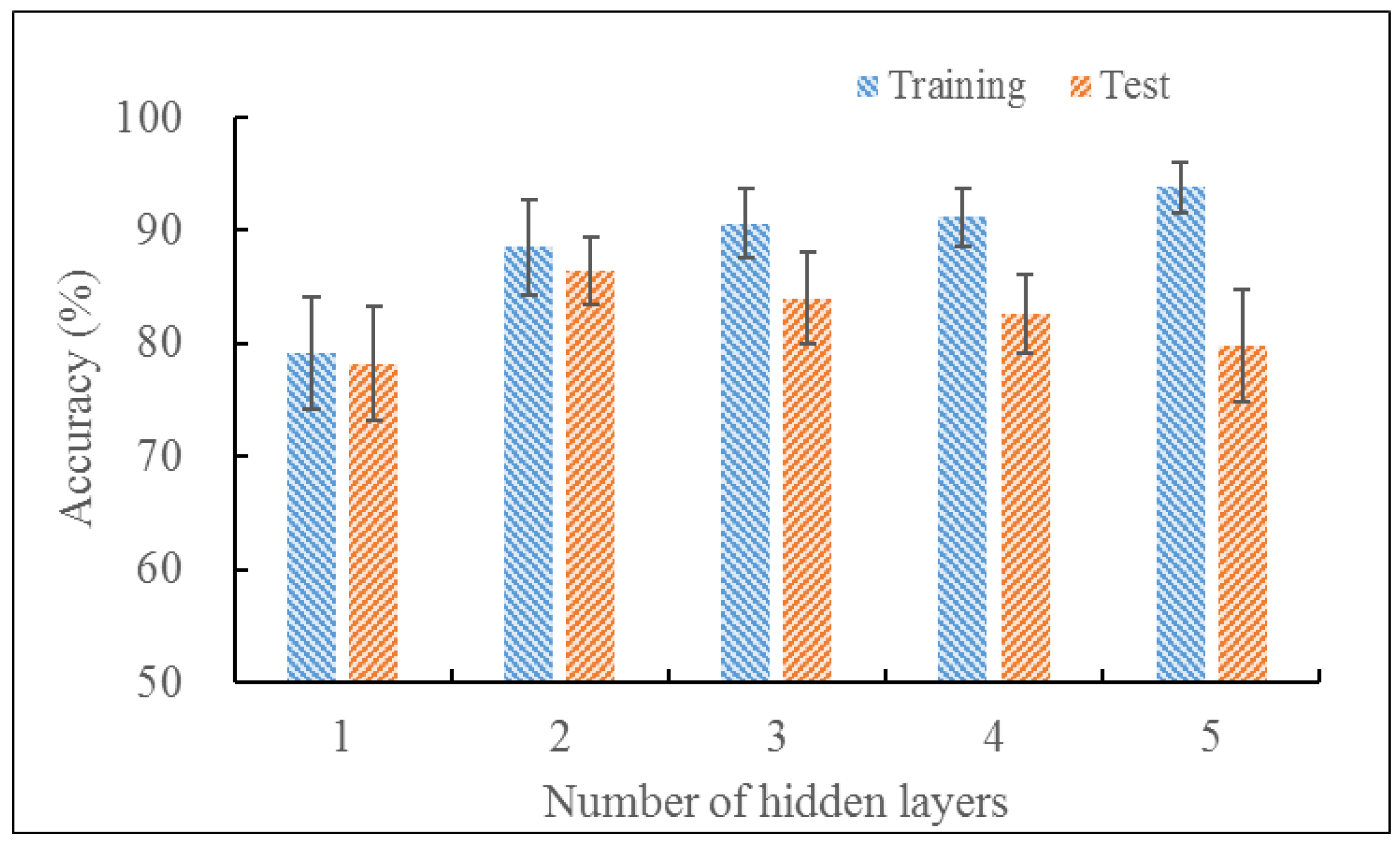
In this section, the characteristic indexes of fNIRS data are utilized as the input to the SDAE model, that is, the input dimension is 864 (108 × 8). The fatigue states were used as the output of the model, that is, the output dimension is two. In order to achieve the best recognition performance, the number of hidden layers was set to 1, 2, 3, 4, and 5, respectively. The number of neurons in the hidden layer was set to 864. The learning rate, the noise rate, the number of iterations, and the batch size were set to 0.1, 0.1, 15, and 4, respectively. The input data were classified, and the classification results are exhibited in Figure 9. With the increase in the number of hidden layers, the identification accuracy rate of the training set grew increasingly high. However, when the number of hidden layers was greater than two, the identification accuracy rate of the test set decreased instead of increasing. When the number of hidden layers was 2, the recognition rate of the network for the training set reached 88.52% and the identification accuracy rate of the network for the test set reached 86.46%. At this point, the accuracy of the test set was the highest. Therefore, two was chosen as the number of hidden layers.

3.3.2. Number of Nodes in the Hidden Layer

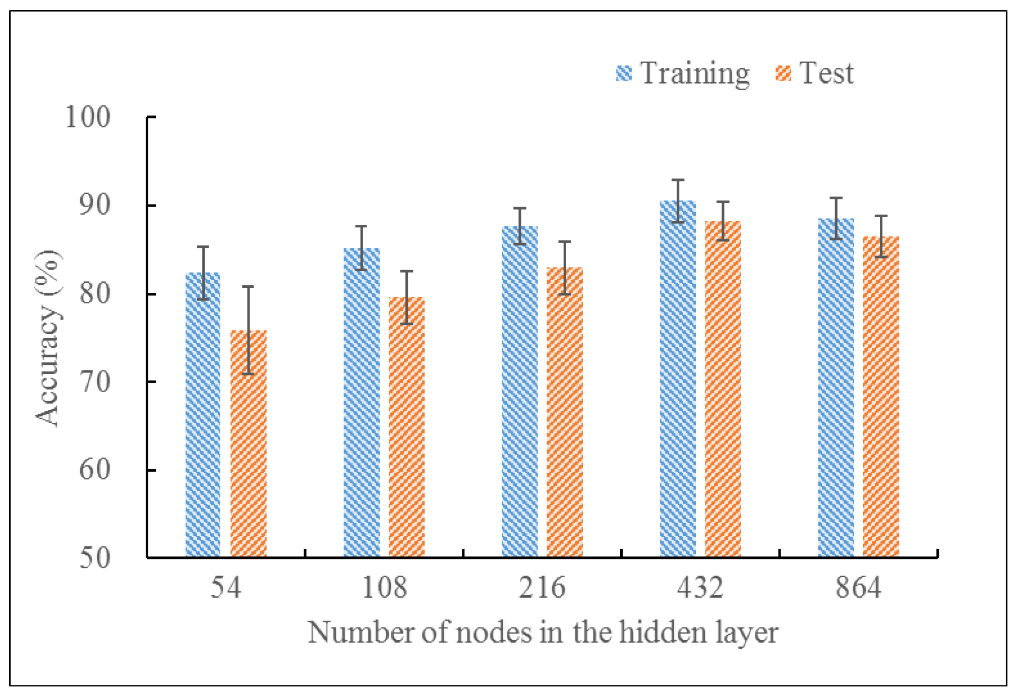
The number of hidden layer nodes was determined on the basis of determining the number of hidden layers. The number of neurons in the first hidden layer of SDAE indicated the feature dimension automatically extracted during the pre-training of the first DAE. Usually, the number of nodes in the hidden layer of SDAE is less than the number of nodes in the input layer. In this study, the number of neurons in the first hidden layer was set to 864, 432, 216, 108, and 54, respectively. The number of neurons in the second hidden layer was 1/2 of the first hidden layer. The networks were trained and tested. Results are illustrated in Figure 10. When the number of neurons in the first hidden layer was 432, the network had the highest accuracy on the training set and test set and the accuracy rate on the test set was 88.19%. Therefore, the number of neurons in the first hidden layer was 432.

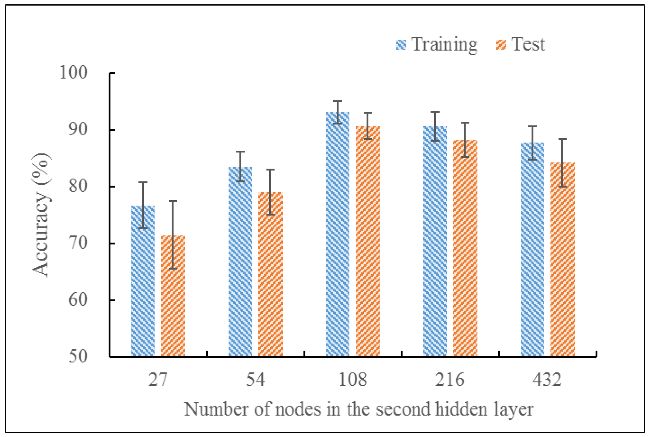
On the basis of choosing the number of neurons in the first hidden layer, the effect of the number of neurons in the second hidden layer on the results of SDAE fatigue identification accuracy is analyzed. The number of neurons in the second hidden layer was set to 27, 54, 108, 216, and 432, respectively. The accuracy results of the training set and test set are revealed in Figure 11. When the number of neurons in the second hidden layer reached 108, the accuracy rate of the training set and test set were 93.06% and 90.63%, respectively. Therefore, 108 was chosen as the number of the second hidden layer neurons after comprehensive consideration.

3.3.3. Noise Rate

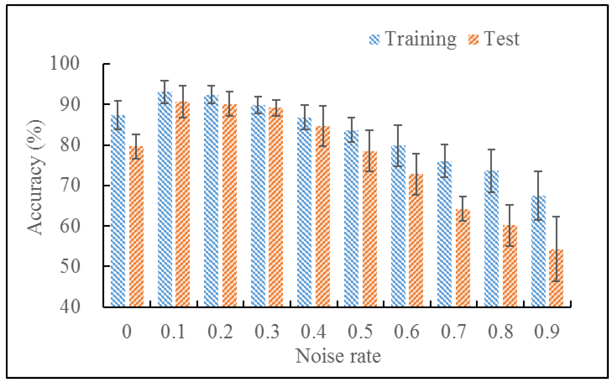
The noise rate indicates the proportion of noise added to the SDAE samples during the pre-training process. The larger the noise rate, the larger the proportion of noise added during the pre-training process. The optimal noise rate was selected through multiple trials, as shown in Figure 12. When the noise ratio was 0.1, the identification accuracy rate of the network was the highest and the identification accuracy rate of the training set and test set were 93.06% and 90.63%, respectively. Therefore, the noise rate was set to 0.1.

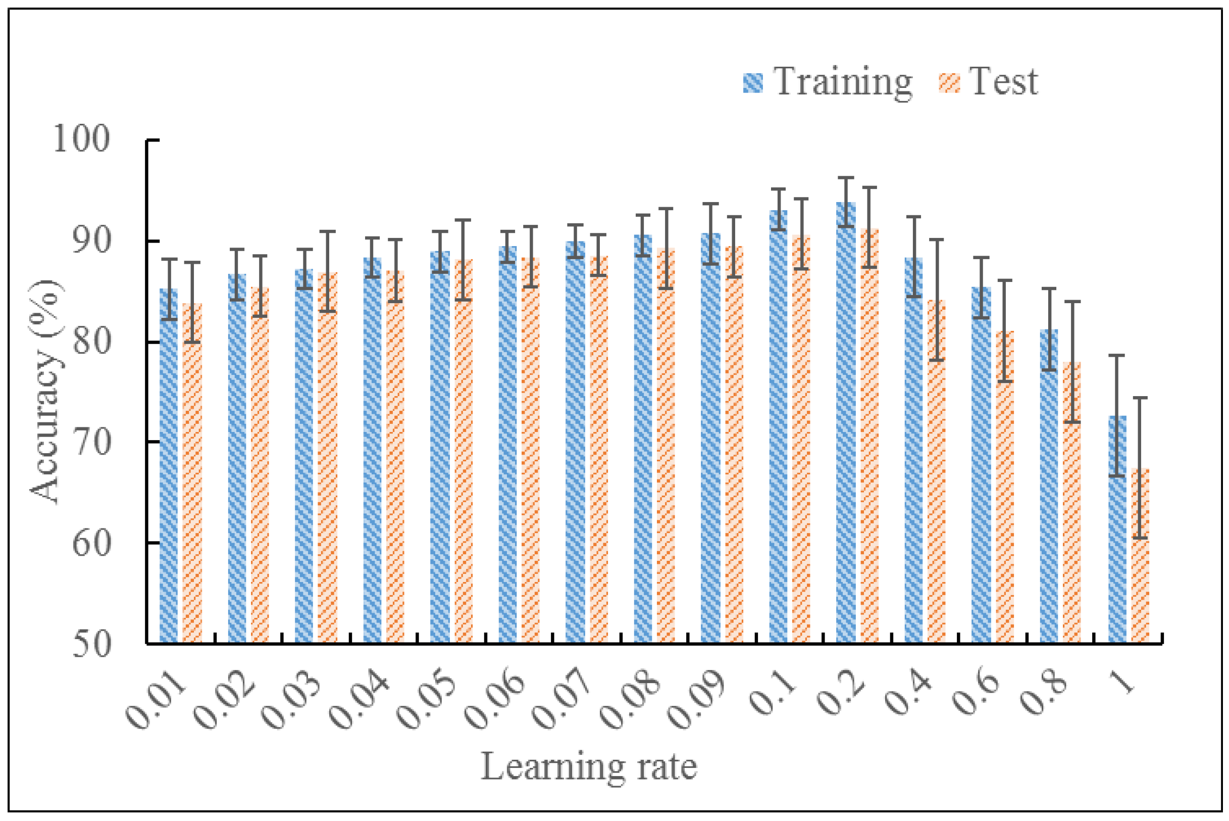
3.3.4. Learning Rate

The accuracy rates of the training set and test set under different learning rates are displayed in Figure 13. When the learning rate was 0.2, the network had the highest identification accuracy rate. The identification accuracy rate of the training set and test set were 93.89% and 91.32%, respectively. Combining the accuracy results of the training set and test set, 0.2 was chosen as the learning rate of the network.

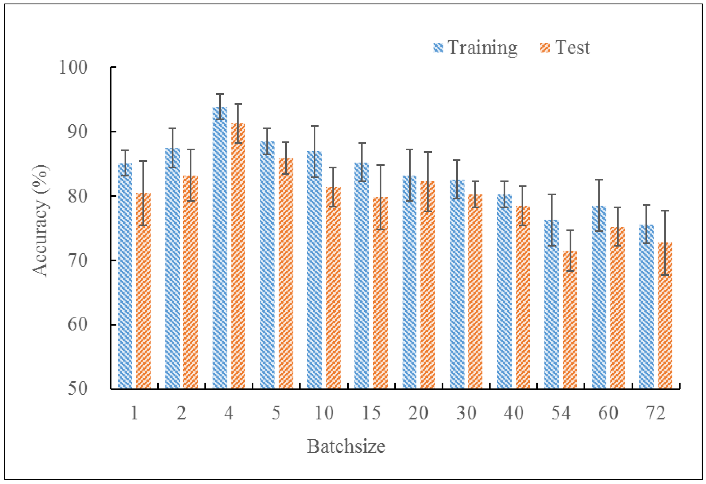
3.3.5. Batch Size

Batch size represents the number of samples loaded into the neural network at a time. The number of batch size must be evenly divisible by the number of training set. Figure 14 shows the relationship between different batch size and identification accuracy rate. When the batch size was 4, the identification accuracy rate of the test set was 91.32%. Therefore, the parameter batch size was set to four.

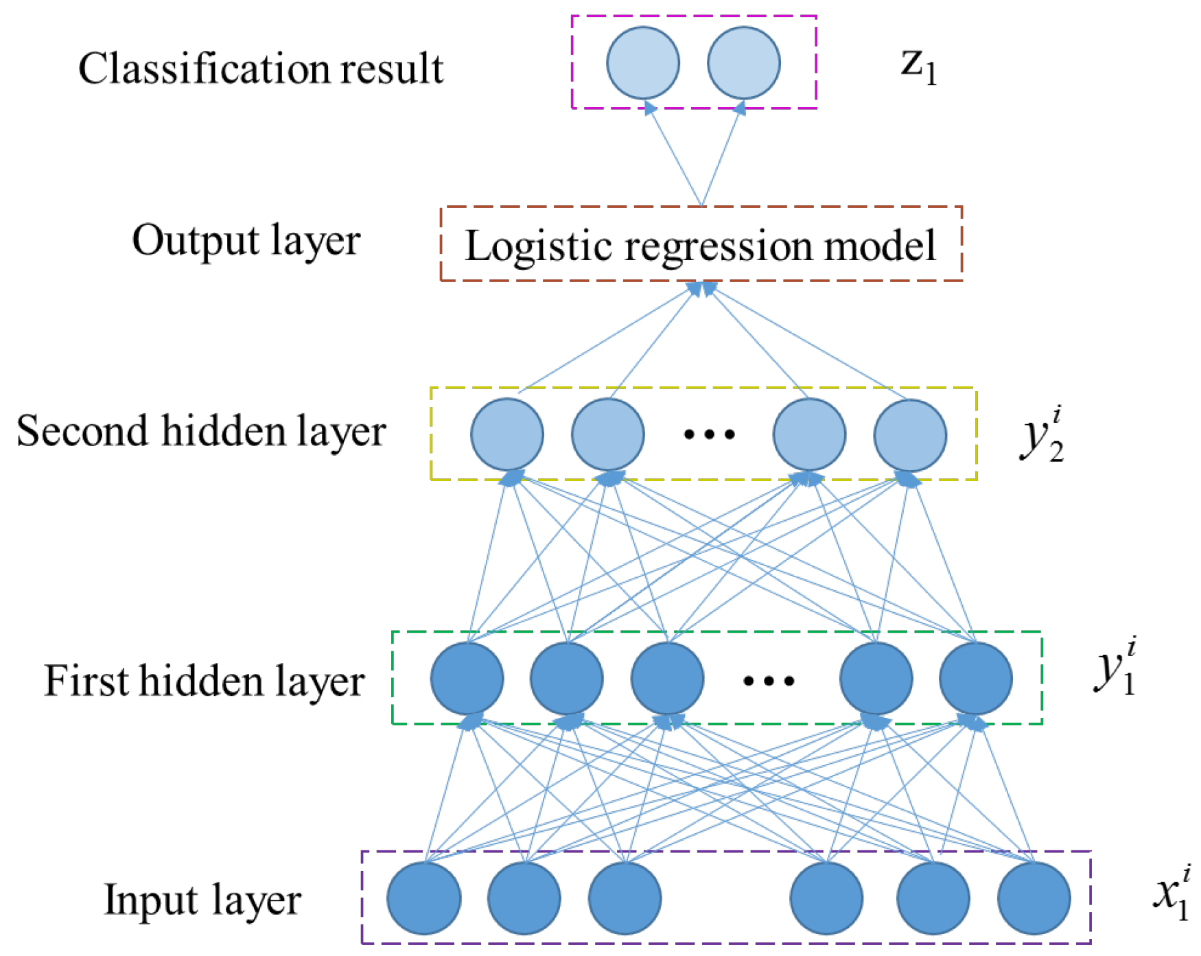
The optimal structure of the trained SDAE neural network is 864-432-108-2, which means that the SDAE neural network has a four-layer of structure, as seen in Figure 15. The input layer is used to input data. The first and the second hidden layers are used for dimensionality reduction and feature extraction. The output layer is utilized for outputting the results. The noise rate, learning rate, and batch size are 0.1, 0.2, and 4, respectively. The accuracy rate of SDAE model training set and test set are 93.89% and 91.32%, respectively.

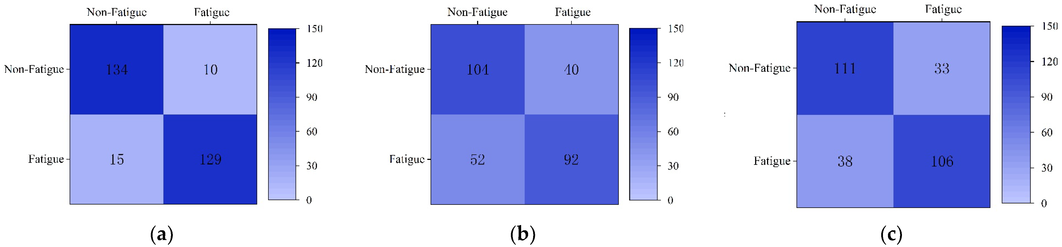
3.4. Model Performance Evaluation

In this section, the identification results of the SDAE model are compared with those of the traditional classification models SVM and LDA to verify the accuracy and effectiveness of the models. The training set was adopted to train SVM and LDA, respectively. In addition, the test set was used to test SVM and LDA models. The confusion matrix of the SDAE model, SVM model, and LDA model are shown in Figure 16 and the results of the identification accuracy rates are found in

Table 7. Identification accuracy rates of models.

Model	SDAE	LDA	SVM
Accuracy (%)	91.32	68.06	75.35

.

Figure 16 demonstrates that the accuracy of the SDAE model under two fatigue states is 93.06% and 89.58%, respectively. The accuracy of the LDA model under two fatigue states is 72.22% and 63.89%, respectively. The accuracy of the SVM model under two fatigue states is 77.08% and 73.61%, respectively. The accuracy of the SDAE model is higher than that of the LDA model and the SVM model under two fatigue states.

Table 7 presents the identification accuracy rate of the SDAE model as 23.26% higher than that of the LDA model and 15.97% higher than that of the SVM model. Therefore, the pilot fatigue identification model based on the SDAE model established in this paper has high identification accuracy.

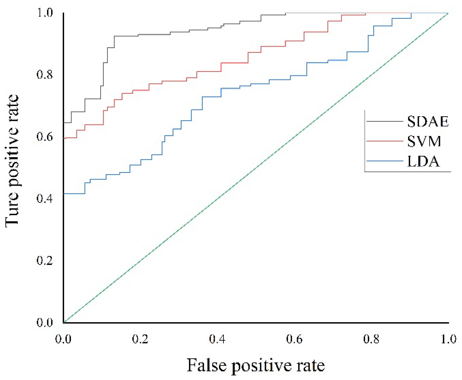
In order to further evaluate the classification performance of the models, four indicators are used in our study: precision rate, recall value, F1 score, and ROC curve. The calculated results of precision, recall value, and F1 score for the SDAE, LDA, and SVM models are indicated in

Table 8. Performance evaluation results of classification models.

Model	Precision (%)	Recall (%)	F1-Score (%)
SDAE	91.32	91.37	91.34
LDA	68.06	68.18	68.12
SVM	75.35	75.38	75.36

, and the receiver operating characteristic curve (ROC) is shown in Figure 17.

Table 8 demonstrates that compared with the LDA model and the SVM model, the SDAE model has higher accuracy, recall value, and F1 score, indicating that the classification precision and the sensitivity of the SDAE model are higher.

As can be seen from Figure 17, three curves are located on the upper left of the 45° diagonal and deviate from the 45° diagonal. However, the SDAE model curve is closer to the (0,1) point than the LDA and SVM model curves, indicating that the SDAE model performs better.

Based on the above accuracy rate, precision rate, recall value, F1 score and ROC curve results, the SDAE model is superior to the LDA model and the SVM model. The SDAE model can effectively identify the two fatigue states of the pilot.

4. Discussion

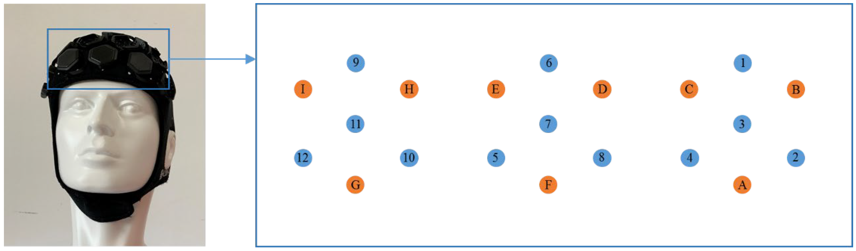
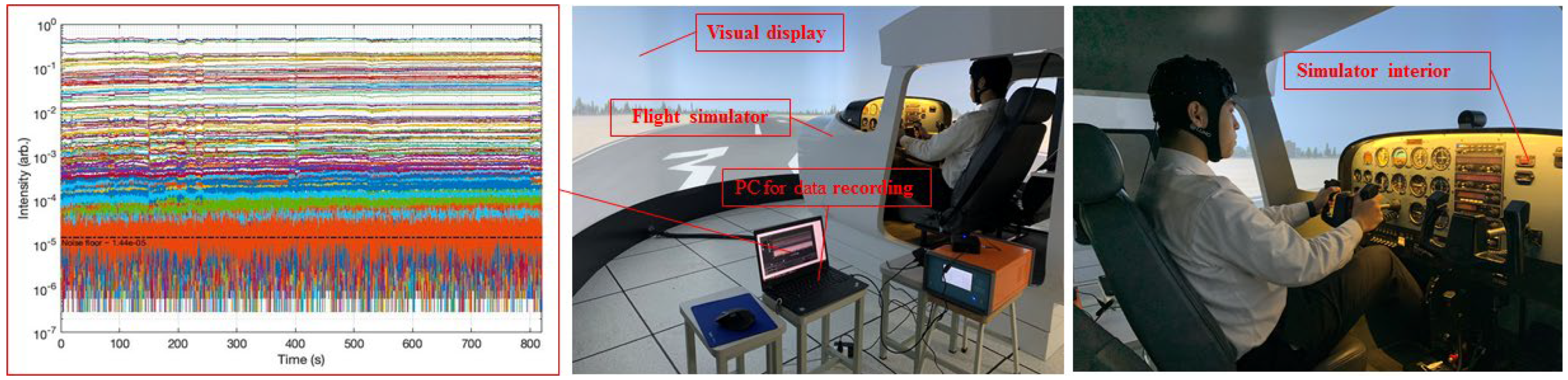
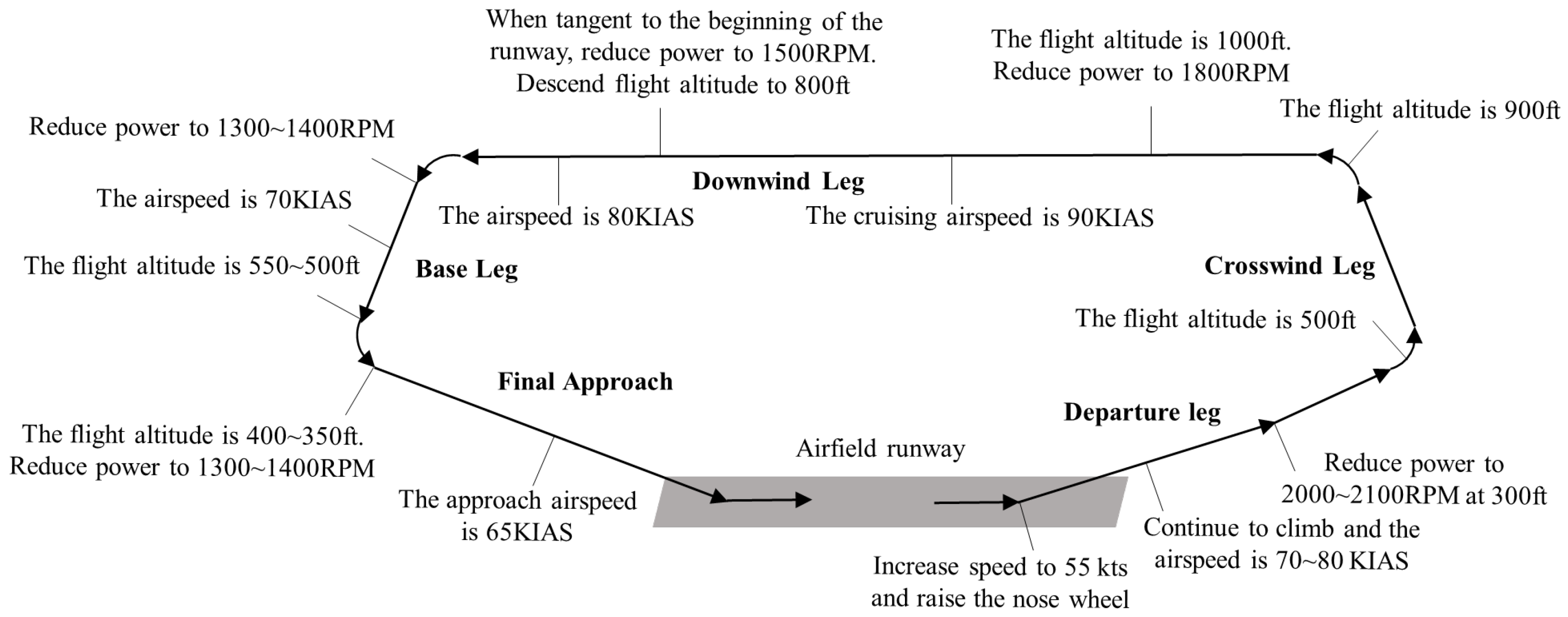
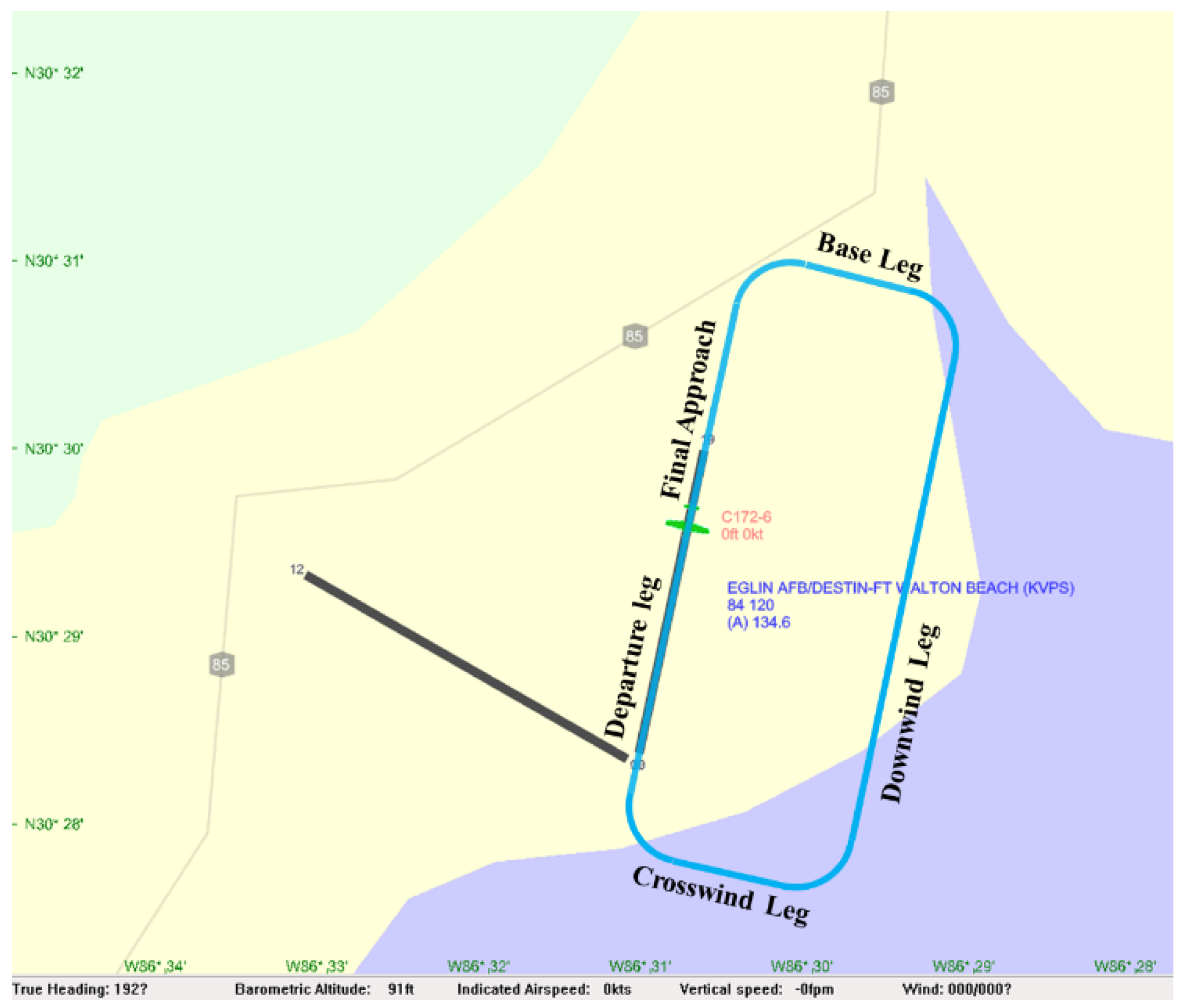
In order to establish the identification model of the pilots’ fatigue state, the pilots were selected as participants. The airfield traffic pattern was selected as the flight task, and the wireless wearable near-infrared device was selected as the data acquisition device. The flight simulation experiment had less interference from the pilot operation and a low cost of data acquisition. Therefore, the obtained fNIRS data are of great significance for studying the identification of pilots’ fatigue status and the effect of fatigue on pilots’ cognitive activities.

The fNIRS signals from the prefrontal lobe of the pilots’ brains were acquired. The results of the study show that the degree of brain fatigue can be reflected by the fNIRS data from the prefrontal lobe of the brain. This is consistent with the results of relevant research [17,42]. Meanwhile, the relative concentration of HbO2 in the fNIRS signal was extracted. The findings suggest that the relative concentration of HbO2 can reflect the degree of brain fatigue, which is consistent with the results of related studies [19,22]. This maintains the consistency of the related research results.

In our study, mean value, variance, standard deviation, kurtosis, skewness, coefficient of variation, peak value, and range of HbO2 for each channel were extracted as the characteristic indexes. Furthermore, the fatigue status of pilots was identified by these characteristic indicators. In related studies, fatigue states have been analyzed by experts and scholars based on indicators such as mean value, variance, skewness, and kurtosis [43]. Our results enrich the research of characteristic indicators of fNIRS.

This means that fNIRS could be a powerful tool for studying fatigue. The relevant characteristics of fNIRS may be indicators of fatigue. Therefore, fNIRS has good prospects in fatigue-related research.

Due to the limitation of time and effort, fatigue was divided into two states in this paper—non-fatigue and fatigue. In future studies, pilots’ fatigue states could be further refined and identified. The experimental participants selected for the experiments in our study were all male pilots, so female pilots could be recruited for the experiments in future research to expand the scope of the study. Thirty pilots were recruited as participants for the flight simulation experiment in our study, and the number of participants could be increased in future studies to improve reliability by increasing the sample size.

5. Conclusions

In this study, the wearable near-infrared equipment was used to obtain pilots’ fNIRS data in the flight simulation experiment and 1080 valid samples were selected. Eight feature indexes (mean, variance, standard deviation, kurtosis, skewness, standard deviation, coefficient of variation, peak value, and extreme deviation) of HbO₂ of each sample were extracted to establish the feature parameter set. These were used as the input of the SDAE model to train and test the pilots’ fatigue state identification model. The identification accuracy of the SDAE model is 91.32%, which is 23.26% and 15.97% higher than that of the LDA and SVM models, respectively. Therefore, the pilots’ fatigue state identification model based on the SDAE established in this paper has high identification accuracy. The SDAE model proposed in this paper can provide a new theoretical basis for the identification of pilots’ fatigue. This research can provide directions for monitoring and an early warning of pilot fatigue during flight missions by using fNIRS in the future. This is conducive to improving the pilot fatigue risk management system (FRMS) and reduce flight accidents caused by pilot fatigue.

References

1. Rosekind, M.R.; Gregory, K.B.; Co, E.L.; Miller, D.L.; Dinges, D.F. Crew Factors in Flight Operations XII: A Survey of Sleep Quantity and Quality in On-Board Crew Rest Facilities; NASA Ames Research Center: Moffett Field, CA, USA, 2000.
2. Kilic, B. Fatigue Among Student Pilots. Aerosp. Med. Hum. Perform. 2021, 92, 20–24. [Google Scholar] [PubMed]
3. Powell, D. Fatigue Self-Management Strategies and Reported Fatigue in International Pilots. Ergonomics 2004, 47, 461–468. [Google Scholar]
4. Dai, J.; Luo, M.; Hu, W.; Ma, J.; Wen, Z. Developing a fatigue questionnaire for Chinese civil aviation pilots. Int. J. Occup. Saf. Ergon. 2020, 26, 37–45. [Google Scholar] [CrossRef] [PubMed]
5. Luo, Y.; Wu, Q. Pilots’ Brain Cognitive State Inference Based on Remaining Life HSMM. In Proceedings of the 2019 Chinese Control and Decision Conference (CCDC), Nanchang, China, 3–5 June 2019; IEEE: Piscataway, NJ, USA, 2019; pp. 5289–5294. [Google Scholar]
6. Pan, T.; Wang, H.; Si, H.; Li, Y.; Shang, L. Identification of Pilots’ Fatigue Status Based on Electrocardiogram Signals. Sensors 2021, 21, 3003. [Google Scholar] [CrossRef]
7. Wu, E.Q.; Lin, C.T.; Zhu, L.M.; Tang, Z.R.; Jie, Y.W.; Zhou, G.R. Fatigue Detection of Pilots’ Brain Through Brains Cognitive Map and Multilayer Latent Incremental Learning Model. IEEE Trans. Cybern. 2021, 1–13. [Google Scholar]
8. Diaz-Piedra, C.; Rieiro, H.; Suarez, J.; Rios-Tejada, F.; Catenae, A.; Stasi, L. Fatigue in the Military: Towards a Fatigue Detection Test Based on the Saccadic Velocity. Physiol. Meas. 2016, 37, 62–75. [Google Scholar] [CrossRef]
9. Naeeri, S.; Manda, S.L.; Kang, Z. Analyzing Pilots’ Fatigue for Prolonged Flight Missions: Multimodal Analysis Approach Using Vigilance Test and Eye Tracking. Proc. Hum. Factors Ergon. Soc. Annu. Meet. 2019, 63, 111–115. [Google Scholar] [CrossRef]
10. Morris, T.L.; Miller, J.C. Electrooculographic and Performance Indices of Fatigue During Simulated Flight. Biol. Psychol. 1996, 42, 343–360. [Google Scholar] [CrossRef]
11. Di Stasi, L.L.; McCamy, M.B.; Martinez-Conde, S.; Gayles, E.; Hoare, C.; Foster, M.; Catena, A.; Macknik, S.L. Effects of Long and Short Simulated Flights on the Saccadic Eye Movement Velocity of Aviators. Physiol. Behav. 2016, 153, 91–96. [Google Scholar] [CrossRef] [Green Version]
12. Perhinschi, M.; Smith, B.; Betoney, P. Development of Pilot Fatigue Detection Schemes Based on Aircraft Sensor Measurements. In Proceedings of the AIAA Modeling & Simulation Technologies Conference & Exhibit, Hilton Head, SC, USA, 20–23 August 2007; American Institute of Aeronautics and Astronautics: New York, NY, USA, 2008; pp. 1–12. [Google Scholar]
13. Dillard, M.B.; Orhan, U.; Letsu-Dake, E. Nonintrusive pilot fatigue monitoring. In Proceedings of the IEEE/AIAA 35th Digital Avionics Systems Conference (DASC), Sacramento, CA, USA, 25–29 September 2016; IEEE: New York, NY, USA, 2016; pp. 1–6. [Google Scholar]
14. Wu, E.Q.; Zhou, M.C.; Hu, D.; Zhu, L.; Tang, Z.; Qiu, X. Self-Paced Dynamic Infinite Mixture Model for Fatigue Evaluation of Pilots’ Brains. In IEEE Transactions on Cybernetics; IEEE: Piscataway, NJ, USA, 2020; pp. 1–16. [Google Scholar]
15. Wu, E.Q.; Deng, P.Y.; Qu, X.Y.; Tang, Z.; Zhang, W.M.; Zhu, L.M.; Re, H.; Zhou, G.R.; Sheng, R.S.F. Detecting Fatigue Status of Pilots Based on Deep Learning Network Using EEG Signals. IEEE Trans. Cogn. Dev. Syst. 2021, 13, 575–585. [Google Scholar] [CrossRef]
16. Hanakova, L.; Socha, V.; Socha, L.; Lalis, L.; Kraus, J.; Malich, T. The Influence of Fatigue on Psychophysiological Indicators During 24 Hours Testing of Pilots. In Proceedings of the 2019 IEEE 17th World Symposium on Applied Machine Intelligence and Informatics (SAMI), Herlany, Slovakia, 24–26 January 2019; IEEE: New York, NY, USA, 2019; pp. 181–186. [Google Scholar]
17. Xu, B.; Wu, Q.; Xi, C.; He, R. Recognition of the Fatigue Status of Pilots Using BF-PSO Optimized Muti-class GP Classification with sEMG Signals. Reliab. Eng. Syst. Saf. 2020, 199, 106930. [Google Scholar]
18. Wu, Q.; Chen, X.; Ding, L.; Wei, C. Classification of EMG Signals by BFA-Optimized GSVCM for Diagnosis of Fatigue Status. IEEE Trans. Autom. Sci. Eng. 2017, 14, 915–930. [Google Scholar]
19. Dehais, F.; Duprès, A.; Flumeri, G.D.; Verdiere, K.; Roy, R. Monitoring Pilot’s Cognitive Fatigue with Engagement Features in Simulated and Actual Flight Conditions Using an Hybrid fNIRS-EEG Passive BCI. In Proceedings of the International Conference on Systems, Man, and Cybernetics, Prague, Czech Republic, 9–12 October 2022; IEEE: Piscataway, NJ, USA, 2018; pp. 544–549. [Google Scholar]
20. Pan, Y.; Borragán, G.; Peigneux, P. Applications of functional near-infrared spectroscopy in fatigue, sleep deprivation, and social cognition. Brain Topogr. 2019, 32, 998–1012. [Google Scholar] [CrossRef] [PubMed] [Green Version]
21. Lin, C.T.; King, J.T.; Chuang, C.H.; Ding, W.; Wang, Y.K. Exploring the Brain Responses to Driving Fatigue Through Simultaneous EEG and fNIRS Measurements. Int. J. Neural Syst. 2019, 30, 1950018. [Google Scholar] [PubMed]
22. Zhao, Y. Research on Fatigue Driving by Using Absolutely Detectable of Brain Imaging of Near-Infrared Spectroscopy; University of Electronic Science and Technology of China: Chengdu, China, 2015. [Google Scholar]
23. Xu, L.; Wang, B.; Xu, G.; Wang, W.; Liu, Z.; Li, Z. Functional Connectivity Analysis Using fNIRS in Healthy Subjects During Prolonged Simulated Driving. Neurosci. Lett. 2017, 640, 21–28. [Google Scholar] [CrossRef]
24. Li, Z.; Zhang, M.; Zhang, X.; Dai, S.; Yu, X.; Wang, Y. Assessment of Cerebral Oxygenation During Prolonged Simulated Driving Using Near Infrared Spectroscopy: Its Implications for Fatigue Development. Eur. J. Appl. Physiol. 2009, 107, 281–287. [Google Scholar] [CrossRef]
25. Khan, M.J.; Hong, K.S. Passive BCI Based on Drowsiness Detection: An fNIRS Study. Biomed. Opt. Express 2015, 6, 4063–4078. [Google Scholar] [CrossRef] [Green Version]
26. Nguyen, T.; Ahn, S.; Jang, H.; Jun, S.C.; Kim, J.G. Utilization of a Combined EEG/NIRS System to Predict Driver Drowsiness. Sci. Rep. 2017, 7, 43933. [Google Scholar] [CrossRef] [Green Version]
27. Zhang, Z.; Jiang, J.; Fu, J.; Cao, Y.; Jiao, X. Multi physiological mental fatigue detection based on the functional near infrared spectroscopy. Chin. J. Sci. Instrum. 2017, 38, 1345–1352. [Google Scholar]
28. Akerstedt, T.; Gillberg, M. Subjective and Objective Sleepiness in the Active Individual. Int. J. Neurosci. 1990, 52, 29–37. [Google Scholar] [CrossRef]
29. Ingre, M.; Akerstedt, T.; Peters, B.; Anund, A.; Kecklund, G. Subjective Sleepiness, Simulated Driving Performance and Blink Duration: Examining Individual Differences. J. Sleep Res. 2006, 15, 47–53. [Google Scholar] [CrossRef] [PubMed]
30. Yan, Y.; Yuan, H.; Yang, X.; Liu, G.; Guo, Z.; Wang, L. Relationship Model of Monotonous Road Environment and Driving Fatigue Based on Multi-Source Data. China J. Highw. Transp. 2021, 34, 156–167. [Google Scholar]
31. Strangman, G.; Culver, J.P.; Thompson, J.H.; Boas, D.A. A Quantitative Comparison of Simultaneous BOLD fMRI and NIRS Recordings during Functional Brain Activation. NeuroImage 2002, 17, 719–731. [Google Scholar] [CrossRef]
32. Homae, F.; Watanabe, H.; Nakano, T.; Taga, G. Prosodic Processing in the Developing Brain. Neurosci. Res. 2007, 59, 29–39. [Google Scholar] [CrossRef] [PubMed]
33. Hoshi, Y.; Kobayash, N.; Tamura, M. Interpretation of Near-infrared Spectroscopy Signals: A Study with a Newly Developed Perfused Rat Brain Model. J. Appl. Physiol. 2001, 90, 1657–1662. [Google Scholar] [CrossRef] [Green Version]
34. Wang, L.; Sang, L.; Zhang, Y.; Zhang, J.; Nian, Y.; Li, P.; Qiao, M.; Qiu, M. Near infrared brain functional imaging of working memory in health young individuals. J. Third Mil. Med. Univ. 2019, 41, 2061–2068. [Google Scholar]
35. Cooper, R.J.; Selb, J.; Gagnon, L.; Phillip, D.; Schytz, H.W.; Lversen, H.K.; Ashina, M.; Boas, D.A. A Systematic Comparison of Motion Artifact Correction Techniques for Functional Near-infrared Spectroscopy. Front. Neurosci. 2012, 6, 147. [Google Scholar] [CrossRef] [Green Version]
36. Coyle, S.; Ward, T.; Markham, C.; McDarby, G. On the Suitability of Near-infrared (NIR) Systems for Next-generation Brain-computer Interfaces. Physiol. Meas. 2004, 25, 815–822. [Google Scholar] [CrossRef] [Green Version]
37. Jiao, X.; Bai, J.; Chen, S.; Li, Q. Near infrared Spectroscopy Signal Processing for Interfacing Brain Function. In Proceedings of the IEEE International Conference on Virtual Environments Human-Computer Interfaces and Measurement Systems (VECIMS), Tianjin, China, 2–4 July 2012; IEEE: Piscataway, NJ, USA, 2012; pp. 1–5. [Google Scholar]
38. Scholkmann, F.; Spichtig, S.; Muehlemann, T.; Wolf, M. How to Detect and Reduce Movement Artifacts in Near-infrared Imaging using Moving Standard Deviation and Spline Interpolation. Physiol. Meas. 2010, 31, 649–662. [Google Scholar] [CrossRef] [Green Version]
39. Izzetoglu, M.; Devaraj, A.; Bunce, S.; Onaral, B. Motion Artifact Cancellation in NIR Spectroscopy using Wiener Filtering. IEEE Trans. Biomed. Eng. 2005, 52, 934–938. [Google Scholar] [CrossRef]
40. Hong, K.S.; Khan, M.J.; Hong, M.J. Feature Extraction and Classification Methods for Hybrid fNIRS-EEG Brain-Computer Interfaces. Front. Hum. Neurosci. 2018, 12, 246. [Google Scholar] [CrossRef] [PubMed]
41. Vincent, P.; Larochelle, H.; Bengio, Y.; Manzagol, P. Extracting and Composing Robust Features with Denoising Autoencoders. In Proceedings of the Twenty-Fifth International Conference on Machine Learning (ICML 2008), Helsinki, Finland, 5–9 July 2008; ACM: New York, NY, USA, 2008; pp. 1096–1103. [Google Scholar]
42. Chuang, C.H.; Cao, Z.; King, J.T.; Wu, B.S.; Wang, Y.K.; Lin, C.T. Brain Electrodynamic and Hemodynamic Signatures Against Fatigue During Driving. Front. Neurosci. 2018, 12, 181. [Google Scholar] [CrossRef] [PubMed]
43. Verdière Kevin, J.; Roy, R.N.; Dehaisk, F. Detecting Pilot’s Engagement Using fNIRS Connectivity Features in an Automated vs. Manual Landing Scenario. Front. Hum. Neurosci. 2018, 12, 6. [Google Scholar] [CrossRef] [PubMed] [Green Version]
Figure 1. Research architecture diagram.
Aerospace 09 00173 g001
Figure 2. The position of the near-infrared light source and detector.
Aerospace 09 00173 g002
Figure 3. Experimental scene.
Aerospace 09 00173 g003
Figure 4. Schematic diagram of airfield traffic pattern.
Aerospace 09 00173 g004
Figure 5. Schematic diagram of airfield traffic pattern path.
Aerospace 09 00173 g005
Figure 6. Schematic diagram of fNIRS data before and after denoising. (a) fNIRS data before denoising; (b) fNIRS data after denoising.
Aerospace 09 00173 g006
Figure 7. Schematic diagram of the DAE.
Aerospace 09 00173 g007
Figure 8. Schematic diagram of the training process of SDAE.
Aerospace 09 00173 g008
Figure 9. The relationship between the number of hidden layers and recognition rate.
Aerospace 09 00173 g009
Figure 10. Recognition results of different numbers of neurons in the first hidden layer.
Aerospace 09 00173 g010
Figure 11. Accuracy results of different number of neurons in the second hidden layer.
Aerospace 09 00173 g011
Figure 12. Recognition rate under different noise rates.
Aerospace 09 00173 g012
Figure 13. The relationship between learning rate and accuracy rate.
Aerospace 09 00173 g013
Figure 14. The relationship between batch size and accuracy rate.
Aerospace 09 00173 g014
Figure 15. The relationship between batch size and accuracy rate.
Aerospace 09 00173 g015
Figure 16. Confusion matrix of the three classification models. (a) SDAE; (b) LDA; (c) SVM.
Aerospace 09 00173 g016
Figure 17. ROC curves of three models.
Aerospace 09 00173 g017