An End-to-End UAV Simulation Platform for Visual SLAM and Navigation

Abstract

Visual simultaneous localization and mapping (v-SLAM) and navigation of unmanned aerial vehicles (UAVs) are receiving increasing attention in both research and education. However, extensive physical testing can be expensive and time-consuming due to safety precautions, battery constraints, and the complexity of hardware setups. For the efficient development of navigation algorithms and autonomous systems, as well as for education purposes, the ROS-Gazebo-PX4 simulator was customized in-depth, integrated into our previous released research works, and provided as an end-to-end simulation (E2ES) solution for UAV, v-SLAM, and navigation applications. Unlike most other similar works, which can only stimulate certain parts of the navigation algorithms, the E2ES platform simulates all of the localization, mapping, and path-planning kits in one simulator. The navigation stack performs well in the E2ES test bench with the absolute pose errors of 0.3 m (translation) and 0.9 degree (rotation), respectively, for an 83 m length trajectory. Moreover, the E2ES provides an out-of-box, click-and-fly autonomy in UAV navigation. The project source code is opened for the benefit of the research community.

1. Introduction

With the advent of modern artificial intelligence algorithms, multi-rotor unmanned aerial vehicles (UAVs) have become smart agents that can navigate in unknown environments. Given a target destination, UAVs can perceive the environment, reconstruct the environment map, and dynamically plan a trajectory to the target destination. Three types of tool kits have been applied in such scenarios: localization, mapping, and planning. The localization (or named pose estimation) kit utilizes onboard sensor information, such as that provided by a stereo camera, to estimate the vehicle’s six degrees of freedom (DoF) pose in real time. The pose feeds into the flight control unit (FCU) to achieve position–level control. Using the UAV’s pose and sensor inputs (e.g., point cloud input), the mapping kit reconstructs the environment throughout the mission. Typically, the environment is presented by a three-dimensional (3D) occupancy voxel map with Euclidean signed distance information [1]. The path-planning kit identifies the lowest-cost path to the destination, avoids obstacles, and generates a trajectory. That trajectory is then sent to the FCU as part of the time sequence used to navigate the UAV.

Verifying such UAV navigation systems under realistic scenarios can be effort-intensive, and failures during testing may damage the UAVs. To overcome these issues, simulators that provide simulated hardware components, such as perception sensors can be used, as they ease reconfiguration and enhance the flexibility of the environmental setup. Although various UAV simulation tools are currently available, most do not focus on a specific task. For example, flight-dynamic-oriented simulation ignores all environmental information. The simulation used in the visual simultaneous localization and mapping (vSLAM) study simplified the dynamic model of the UAV; the navigation-oriented simulation environment contained 3D information about the environment, but it neglected the features of 3D objects. Some simulation tools [2,3] achieve autonomous navigation to a certain degree, but their flexibility is limited, and their source codes have not been released. Thus, the motivation of this work is to construct an end-to-end simulation (E2ES) environment for research and education purposes. Throughout this paper, ’end-to-end’ refers to the capability of verifying the perception, reaction, and control algorithms in one simulator (Figure 1).

Based on the widely used ROS-Gazebo-PX4 toolchain, we made several improvements to the UAV model, environment, and function plugins to meet the requirement of UAV v-SLAM and navigation (Figure 2). These improvements include: (a) the construction of a simulated world, (b) the customization of UAV models, (c) the addition of a stereo camera model, and (d) the configuration of a vision-based control setup. At the end of this paper, we describe an E2ES for UAV navigation (Figure 3). In summary, the contributions of this work are as follows:

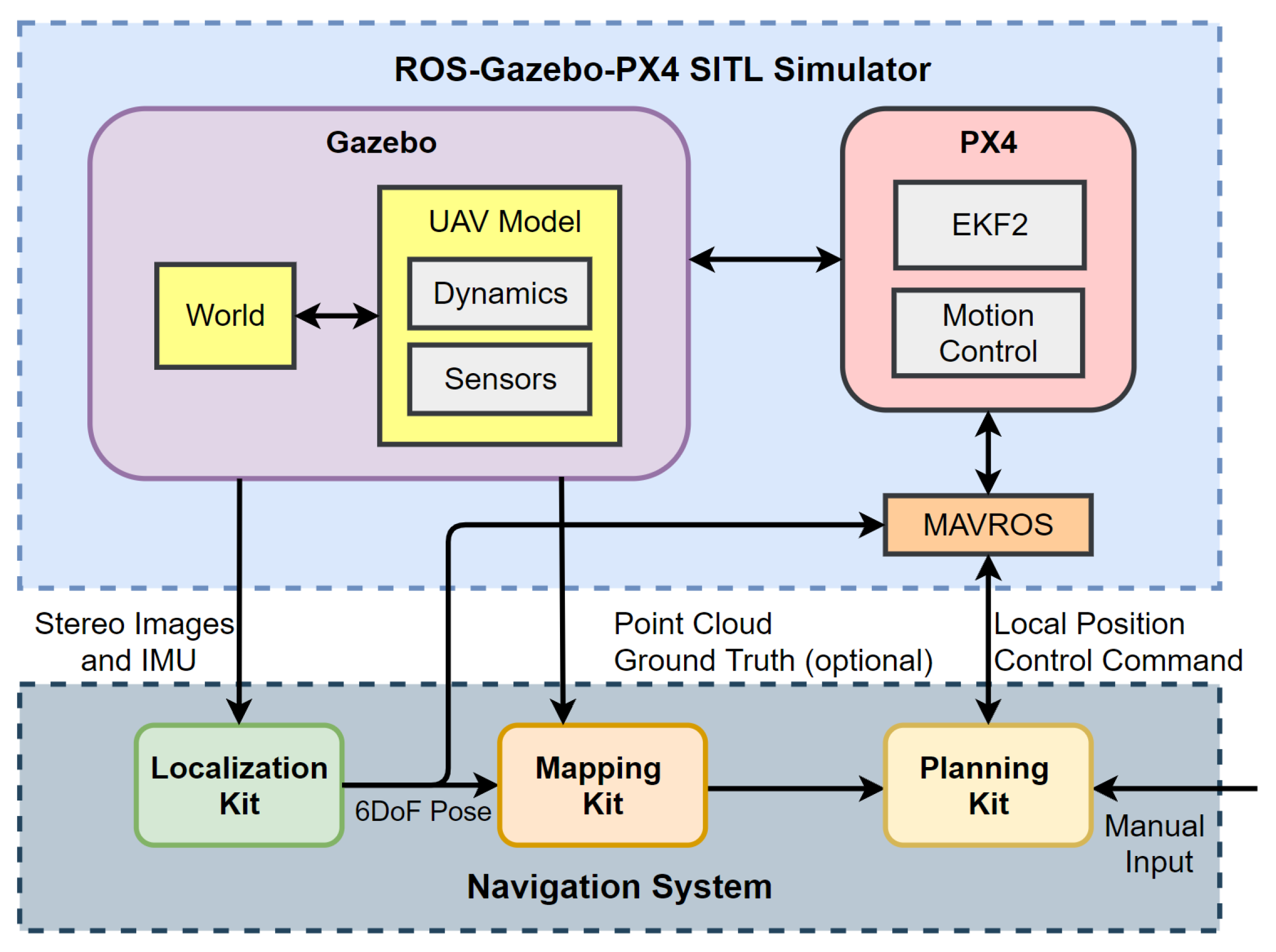
• Customization of the ROS-Gazebo-PX4 simulator in terms of the support of stereo inertial vision estimation, vision feedback control, and ground-truth level evaluation.
• Integration of functions, including localization, mapping, and planning, into tool kits.
• Achievement of click-and-fly level autonomy in the simulation environment.
• Release of the simulation setup, together with the localization kit, mapping kit, and planning kit as open-source tools for the research community (Supplementary Materials).

The remainder of this work is organized as follows. Section 2 describes related works. Section 3 introduces the customized simulation framework, and Section 4 shows the integrated vSLAM and navigation kits. Section 5 shows the simulation results and performance analysis. Finally, Section 6 concludes the paper.

2. Related Works

2.1. UAV Simulators

Depending on the scope of simulation, UAV simulators can be classified into two categories: flight dynamics simulators and environment-integrated simulators. The first type focuses on simulating the dynamics of different UAV platforms, and all environmental information is neglected except for the force of gravity. For example, based on Simulink in MATLAB, Quad-Sim [4] was demonstrated to be suitable to test flight-control algorithms for different dynamic models. Sun et al. [5] developed another Simulink-based simulator that includes a comprehensive aerodynamic model of the tail-sitter vertical take-off and landing UAV. The second type, the environment-integrated simulator (also known as the perception-supported simulator), includes perception sensors and environmental information. Users can access the simulated sensor outputs, such as camera images and the point cloud from the Lidar sensor [6]. For example, Schmittle et al. [7] developed an easy-access web-based UAV testbed for education and research. By applying the containers as a service technology, this simulator is deployed in the cloud; thus, the user does not need a high-performance computer to execute the simulation. Xiao et al. [8] developed a simulation platform called XTDrone. Comparing E2ES with XTDrone, both are based on ROS-Gazebo-PX4 toolchains, which means they have a similar kinetic model and flight controller. However, these two projects focus on solving different problems. XTDrone is focused on providing a general solution for UAV simulation, while the E2ES simulator is focused on providing an out-of-box solution for UAV SLAM and navigation. E2ES is more accessible for achieving full-stack navigation in the loop using its default localization, mapping, and planning tools or customized packages developed by users.

2.2. The UAV vSLAM and Navigation System

Typically, the v-SLAM and the navigation system consist of localization, mapping, and planning modules. The related works are reviewed in sequence.

2.2.1. Localization

The goal of localization is to achieve real-time pose estimations with the onboard computer and sensors. A wide range of methods has been pursued to solve this problem. Most preliminary methods use LiDAR [9,10,11] or cameras to perceive the environment. The LiDAR sensors have a wide detection range and can directly provide high-precision depth information. However, they are also expensive, heavy, and large, which limits the application scenarios of LiDAR on the UAV platform. In contrast, the camera has simple structure, light weight, and cheap price. These features make it very suitable for UAV applications, especially for the limited payload of quadcopter UAVs.

Visual localization (or visual pose estimation) can be realized using either monocular or stereo camera solutions. The monocular solution has the advantages of a simple structure and low weight. However, recovering the scale correctly is a challenge with such a system. Researchers have integrated IMU information [12] or predefined the object pattern [13,14] of the environment to eliminate this problem. Nowadays, stereo camera solutions are available off the shelf. As depth information can be directly extracted from every frame, the accuracy and robustness of this system is better than those of the monocular setup at the cost of a larger stereo data stream. Nevertheless, the use of powerful onboard computers can compensate for this issue.

In the UAV application, visual information is usually fused with the IMU data through either a filter-based framework or an optimization-based framework. Under the filter-based framework, the pose and the landmark are in the system states. IMU inputs propagate the pose states and the relevant con-variance matrices [15,16]. In the optimization-based framework, the IMU engaged through a pre-integration edge [17]. According to Delmerico et al. [18], the optimization-based approach outperforms the filter-based approach in terms of accuracy but requires more computational resources.

2.2.2. Mapping

The mapping system, which provides a foundation for onboard motion planning, is an essential component in the perception–planning–control pipeline. A mapping system needs to optimally trade-off measurement accuracy and the storage overhead. Three types of map have been successfully used in UAV navigation applications: the point cloud map [19], the occupancy map [20], and Euclidean Signed Distance Fields (ESDFs) [21] map.

The point cloud map can be easily obtained by measuring point stitching. However, this type of map is only suitable for high-precision sensors in static environments, because sensor noise and dynamic objects cannot be accessed and modified. Occupancy maps, such as OctoMap [20], store occupancy probabilities in a hierarchical octree structure. The main restrictions of these approaches is their fixed-size voxel grid, which requires a known map size in advance and cannot be dynamically changed [21]. In recent years, ESDF maps have gained popularity [22]. This type of map is suitable for dynamically growing maps and is advantageous in that it can evaluate distance and gradient information with relation to obstacles.

2.2.3. Planning

For UAV route planning, algorithms can be classified into two main categories: sampling-based algorithms [23] and optimization-based algorithms [24]. The rapidly exploring random tree (RRT) algorithm [23] is representative of sampling-based algorithms. In this method, samples are drawn randomly from the configuration space to guide the tree to grow toward the target [25]. The rapidly exploring random graph system [26] is an extension of the RRT algorithm and is asymptotically optimal. Although the sampling-based method is suitable for identifying safe paths, it is not easy for the UAV to follow. The minimum-snap algorithm [24] can be applied to generate a smooth trajectory. It formulates the trajectory generation problem as a quadratic programming problem. By instantly minimizing the cost function, the trajectory can be represented using piece-wise polynomial functions. The cost function includes two terms: the penalty for the trajectory with the potential of collision and the smoothness of the trajectory itself. With optimization-based methods, another way to add constraints to the optimization problem is to first obtain a series of waypoints using a sample search or a grid search and to then optimize the motion primitives to generate a smooth trajectory through the waypoints under the UAV’s dynamic constraints [27]. This approach combines the advantages of the two categories, and its computation efficiency is higher than those of pure optimization-based algorithms. However, the safe radius and other parameters must be tuned carefully.

2.3. UAV SLAM and Navigation Simulations

Some UAV SLAM and navigation simulations have previously been proposed. Zhang et al. [2] proposed a quadrotor UAV simulator integrated with a hierarchical navigation system. Under this approach, the UAV is equipped with two laser scanners and one monocular camera. One laser scanner is mounted on the bottom for altitude control and 3D map construction, while the other is attached to the top for navigation purposes. The monocular camera is attached to a tilting mechanism for target detection and visual guidance. The fused data are then constructed into OctoMap and used to facilitate a trajectory from an A* global path planner. In this approach, the environmental setup is quite simple and does not include visual features, and the navigation is based on Laser SLAM. In Alzugaray et al. [3], a point-to-point planner algorithm was designed to work with the SLAM estimation of a monocular-inertial system. In the simulator, the UAV was flown around the building to reconstruct the environment. However, as the UAV was flown outside the building, obstacle avoidance was not considered in their work.

3. Simulation Platform

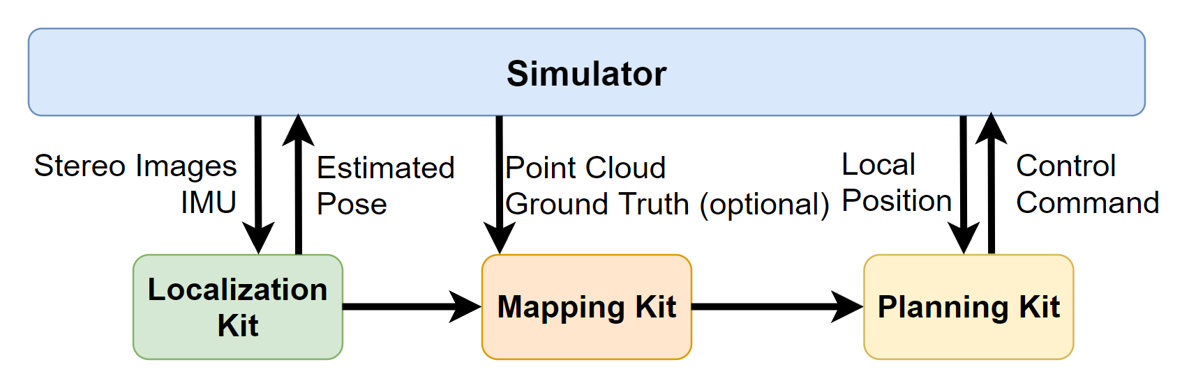
3.1. Overview

The proposed simulation platform is based on the ROS-Gazebo-PX4 toolchain. In the field of robotics, the robot operating system (ROS) [28] is the most convenient platform, because it provides powerful developer tools and software packages from drivers to state-of-the-art algorithms. Moreover, many navigation kits contain the ROS-version package, and it can be integrated conveniently. Moreover, Gazebo [29], which is an open-source robotics simulator, is the most widely used simulator used for ROSs. We selected the widely used open-source UAV autopilot stack, PX4 [30], which supports software in the loop (SITL) simulations.

As shown in Figure 4, the upper part of our simulation is the Gazebo SITL simulator. It has an environmental map, also called "the world", and a simulated UAV model, which supports the dynamic simulation and a series of onboard sensors, including a global positioning system, IMU, barometer, and custom-defined-depth camera sensors. All of these sensors are attached to the UAV through Gazebo plugins. The bottom panel of Figure 4 shows the navigation system. All components are coordinated and communicated through different ROS topics. The communication between the navigation system and PX4 is conducted through MAVROS (http://wiki.ros.org/mavros, accessed on 18 December 2021). In the simulator, PX4 communicates with Gazebo by receiving sensor data from the simulated world and sending motor and actuator commands to the UAV. The extended Kalman Filter-based state estimator and the motion control module run on the PX4 stack.

3.2. The UAV Dynamic Model

The dynamic model in the simulator follows the conventional quadcopter dynamic model, which can be found in general papers on dynamics and control, such as [31,32,33]. The UAV is modeled as a six-DoF rigid body (three DoF in position and three DoF in rotation). The position of the UAV’s center of gravity in the inertial frame is defined by $\mathbf{\xi }={\left[XYZ\right]}^{\mathsf{T}}\in {\mathbb{R}}^3$; the orientation of the UAV is denoted by the rotation matrix from the body frame (B) to the inertial frame (I) ${\mathbf{R}}_B^I\in SO\left(3\right)$. The velocity, as the derivative of position, in the inertial frame is described by $\mathbf{v}={\left[\dot{X}\dot{Y}\dot{Z}\right]}^{\mathsf{T}}\in {\mathbb{R}}^3$, and the angular velocity is denoted by $\mathbf{\omega }$. The kinematics and dynamics of the position and attitude are denoted by:

$$\begin{array}{cc}\hfill \dot{\mathbf{\xi }}& =\mathbf{v},\hfill \\ \hfill m\dot{\mathbf{v}}& ={\mathbf{R}}_B^I{\mathbf{F}}_B,\hfill \\ \hfill {\dot{\mathbf{R}}}_B^I& ={\mathbf{R}}_B^I{\mathbf{\omega }}_{\times },\hfill \\ \hfill \mathbf{I}\dot{\mathbf{\omega }}& =-\mathbf{\omega }\times \left(\mathbf{I}\mathbf{\omega }\right)+{\mathbf{M}}_B,\hfill \end{array}$$

(1)

where m denotes the mass, $\mathbf{I}$ denotes the inertia matrix of the vehicle, and ${\mathbf{\omega }}_{\times }$ denotes the skew-symmetric matrix, such that ${\mathbf{\omega }}_{\times }\mathbf{v}=\mathbf{\omega }\times \mathbf{v}$ for any vector $\mathbf{v}\in {\mathbb{R}}^3$. ${\mathbf{F}}_B$ and ${\mathbf{M}}_B$ are the total force and moment acting on the body frame, respectively. The dynamic simulation of the UAV is achieved by the model in Gazebo. The PX4 SITL simulator handles the inner loop attitude, velocity, and position control. The user commands the UAV in the off-board control mode by sending the target position or velocity command through MAVROS.

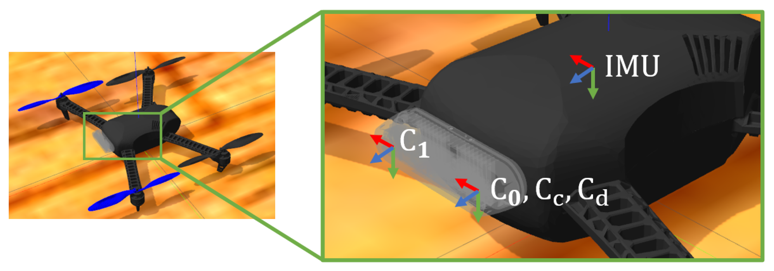
3.3. On-Board Sensors

To improve the 3DR-IRIS model provided by the original PX4 firmware, we added a depth camera and customized the IMU sensor to support the visual–inertial pose estimator. To do this, we introduced the camera and IMU models. The coordinate definition of the body and the IMU are shown in Figure 5.

3.3.1. The Visual Sensor

The visual sensor is based on librealsense_gazebo_plugin (https://github.com/pal-robotics/realsense_gazebo_plugin, accessed on 17 December 2021). The visual sensor in the simulator consists of two gray-scale cameras ($C_0$ and $C_1$), a color camera ($C_c$), and a depth camera ($C_d$). All of these cameras are based on the non-distortion pinhole camera model. The output of the sensors includes two gray-scale images, a color image, a depth image, and a point cloud. All of these outputs are temporally synchronized. The horizon field of view ($HFOV$) and resolution ($width\times height$) define the intrinsic camera parameters ($f_x$, $f_y$, $c_x$, $c_y$) as follows:

$$f_x=f_y=\frac{width}{2·tan(HFOV/2)}$$

(2)

$$c_x=c_x=\frac{width}{2};c_y=\frac{height}{2}.$$

(3)

The installation geometry in the SDFormat (Simulation Description Format) file defines the extrinsic parameters. For convenience, the color camera, the depth camera, and the left pinhole camera were installed in the same link, which means the color image, depth image, left gray-scale image, and point cloud were all aligned.

3.3.2. The IMU

In the simulator, the IMU consists of a three-axis accelerometer and a three-axis gyroscope. The measured angular velocity and acceleration can be described using the following models:

$$\begin{array}{cc}\hfill & {\mathbf{\omega }}_m={\mathbf{\omega }}_{real}+{\mathit{b}}_{\omega }+{\mathit{n}}_{\omega }\hfill \end{array}$$

(4)

$$\begin{array}{cc}\hfill & {\mathit{a}}_m={\mathit{a}}_{real}+{\mathit{b}}_a+{\mathit{n}}_a\hfill \end{array}$$

(5)

$$\begin{array}{cc}\hfill & {\mathit{n}}_{\omega }\sim \mathcal{N}(\mathbf{0},{\mathbf{\sigma }}_{\omega }^2);{\mathit{n}}_a\sim \mathcal{N}(\mathbf{0},{\mathbf{\sigma }}_a^2)\hfill \end{array}$$

(6)

$$\begin{array}{cc}\hfill & {\dot{\mathit{b}}}_{\omega }\sim \mathcal{N}(\mathbf{0},{\mathbf{\sigma }}_{{\omega }_b}^2);{\dot{\mathit{b}}}_a\sim \mathcal{N}(\mathbf{0},{\mathbf{\sigma }}_{a_b}^2),\hfill \end{array}$$

(7)

where ${\mathit{n}}_{\omega }$ and ${\mathit{n}}_a$ refer to the intrinsic noise of the sensor, which follows the Gaussian distribution. Biases, including ${\mathbf{\omega }}_b$ and ${\mathit{a}}_b$, are affected by the temperature and change over time. Slow variations in the sensor biases are modeled using random walk noise in discrete time. That is, the time derivatives of the biases (i.e., ${\dot{\mathit{b}}}_{\omega }$ and ${\dot{\mathit{b}}}_a$) follow the Gaussian distribution. Furthermore, in the IRIS model provided by PX4 firmware, the update rate of the IMU is constrained by the MAVROS. To cross the speed limit, we added another IMU plugin, which publishes IMU information at a rate of 200 Hz.

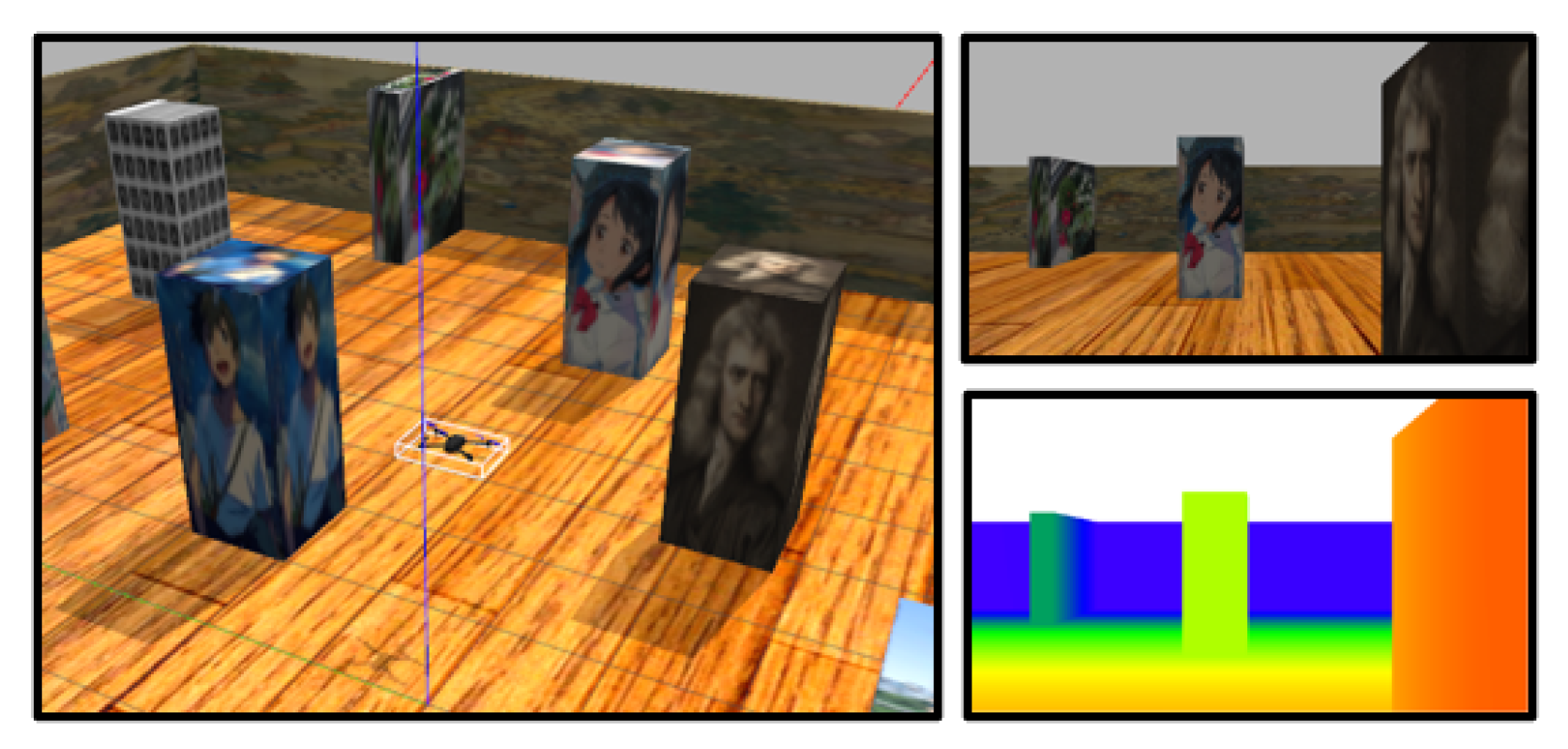
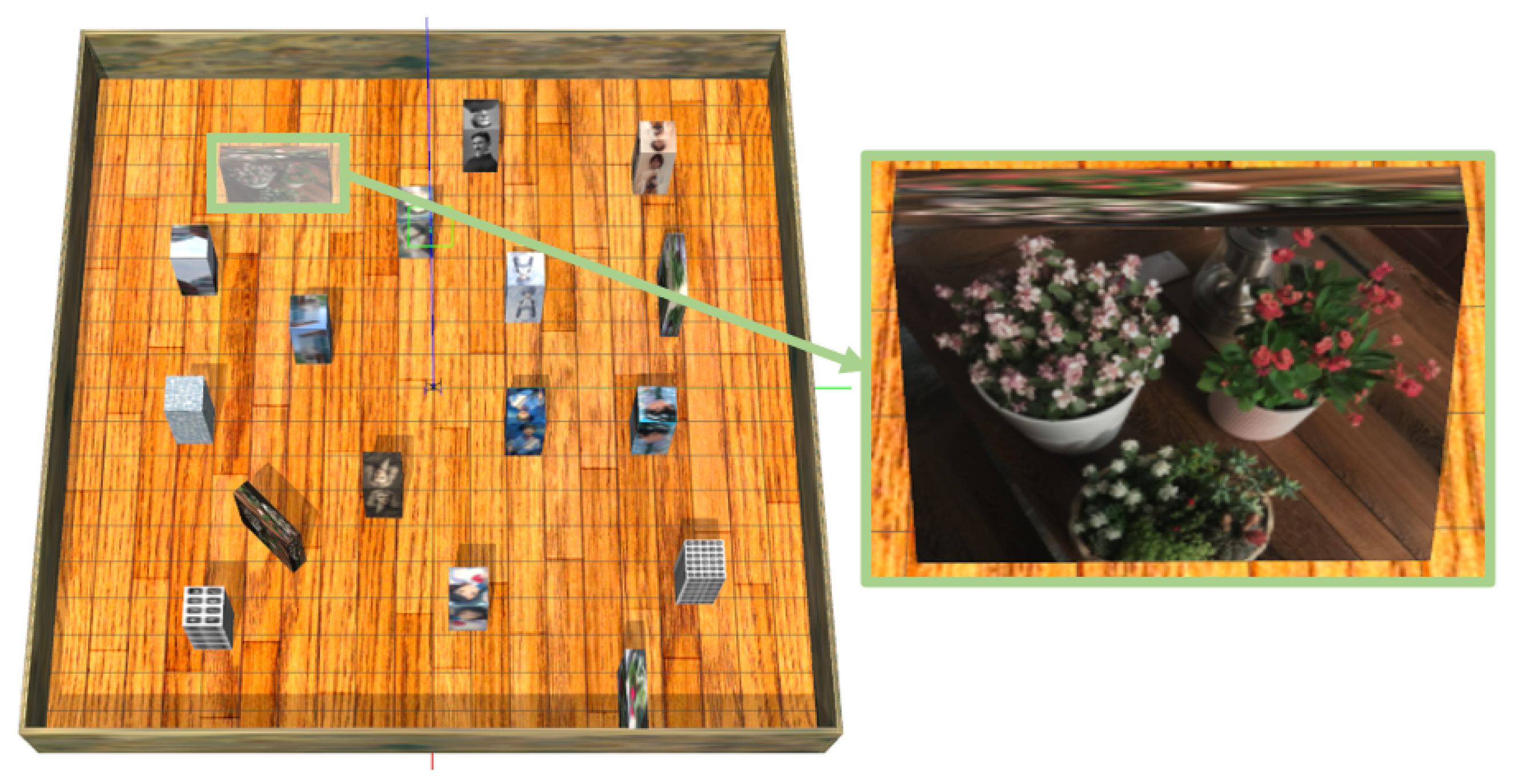
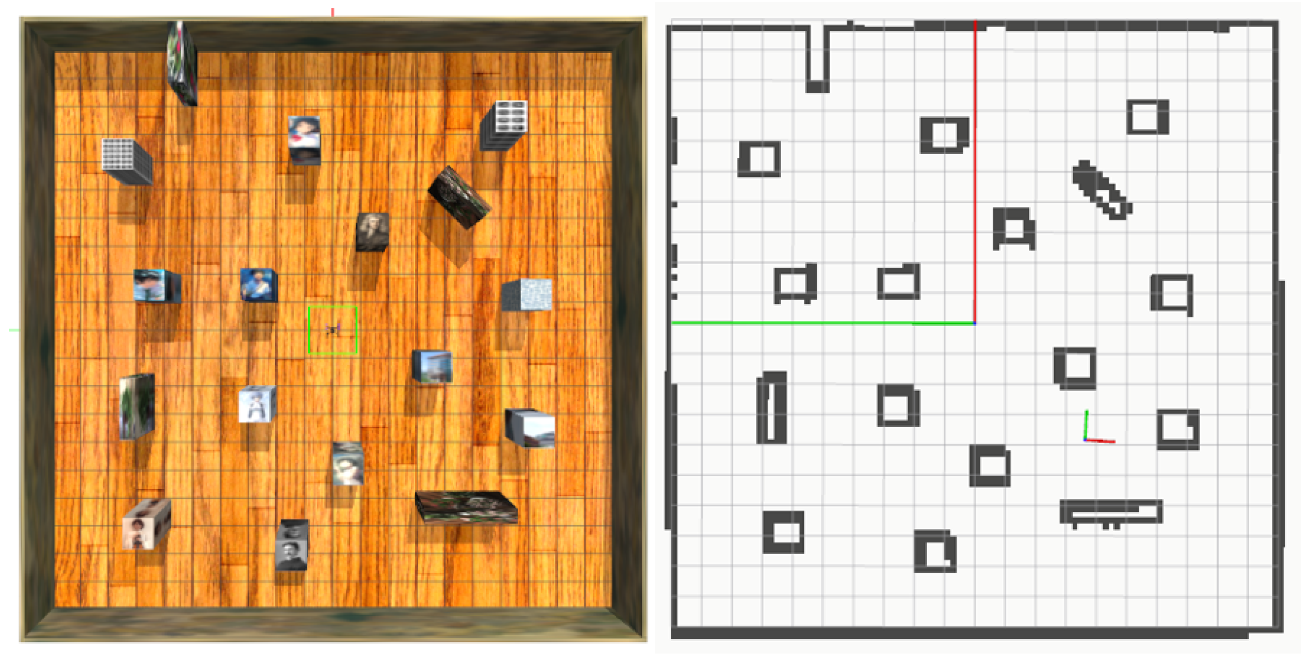
3.4. The Simulation World Setup

First, we added obstacles, such as walls and boxes, into a $20\times 20$ m empty world. Then, to meet the requirements of v-SLAM simulation, we furnished all of these items and the ground plane with various wallpaper, which contained rich visual features, as shown in Figure 6.

4. MAV Navigation Framework

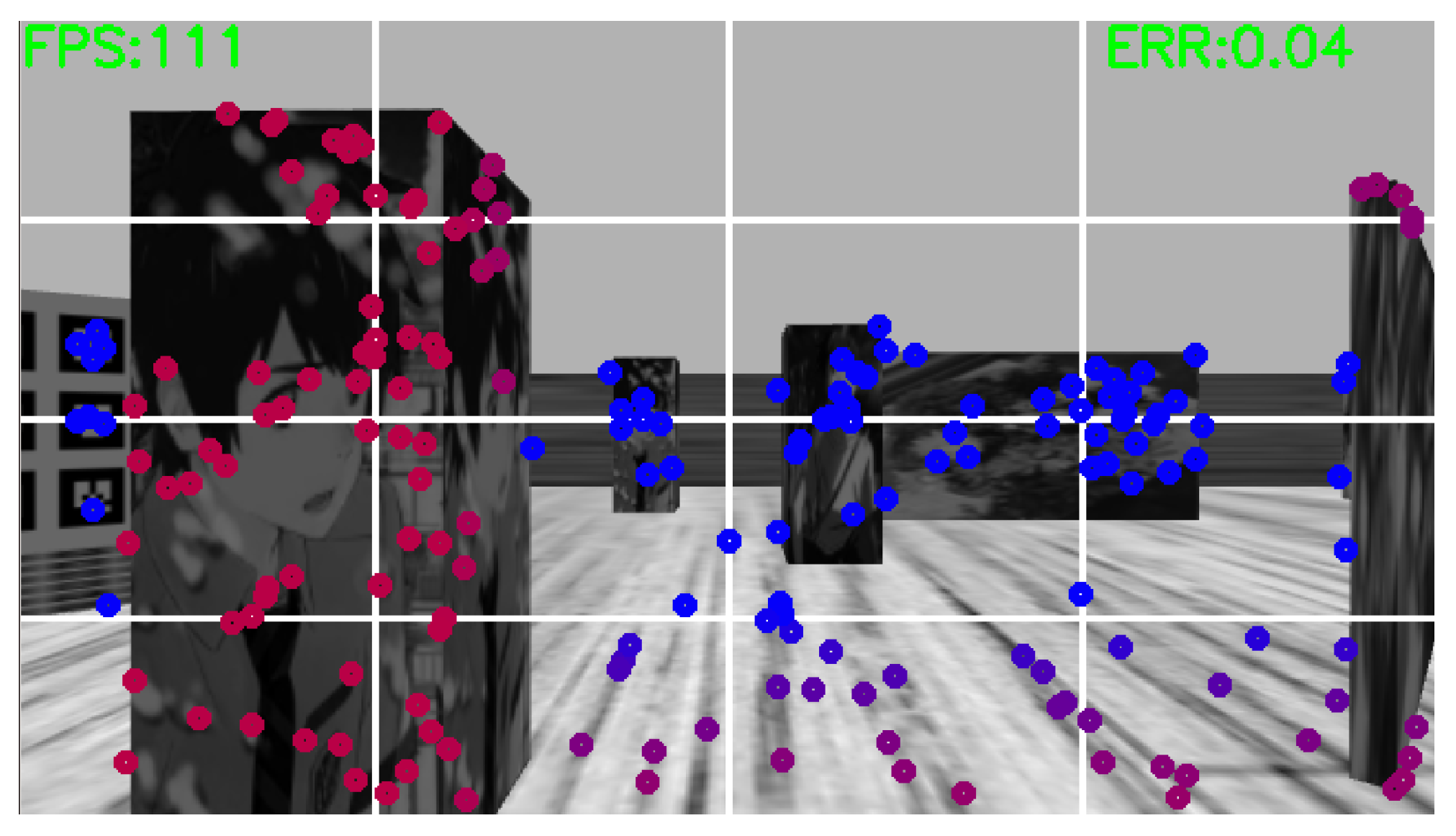
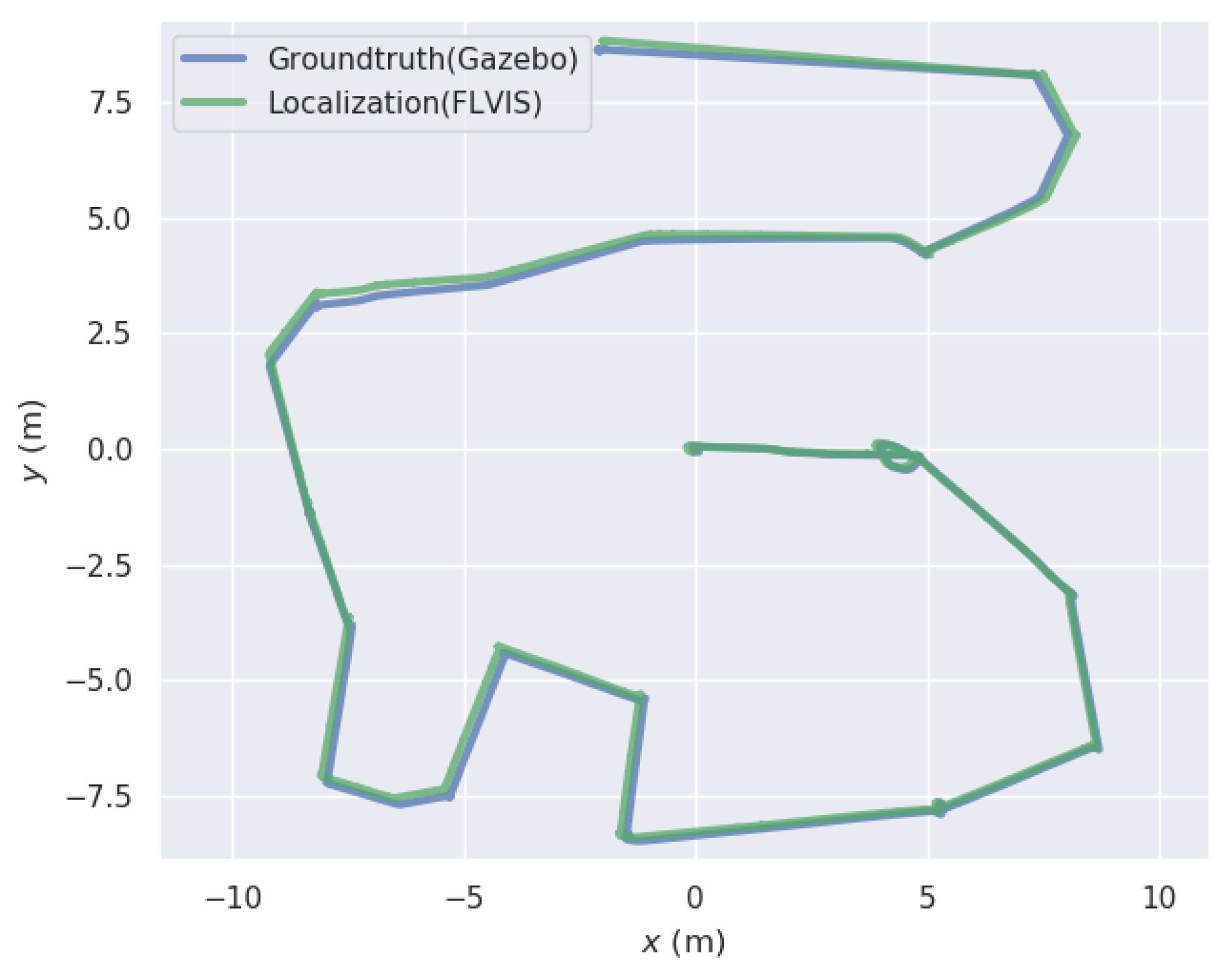
4.1. Localization

For localization, a stereo visual-inertial pose estimator, FLVIS [34], which was developed by our group, was integrated as the localization kit in the proposed simulation platform (Figure 7). Compared with other monocular v-SLAM solutions, the stereo visual-inertial pose estimator has the advantages of robustness, accuracy, and scale consistency. Robustness means that the pose between consecutive visual frames can be estimated by the IMU when visual tracking is lost. Accuracy means that more measurements are fused in the pose estimation process to achieve better accuracy. Scale consistency means that the depth information can be extracted directly from stereo images without any motion. FLVIS uses feedback/feedforward loops to fuse the data from the IMU and stereo/RGB-D camera and to achieve high accuracy in the resource-limited computation platform.

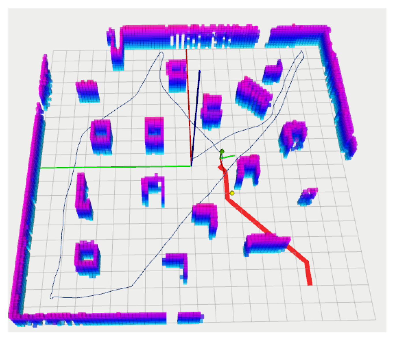
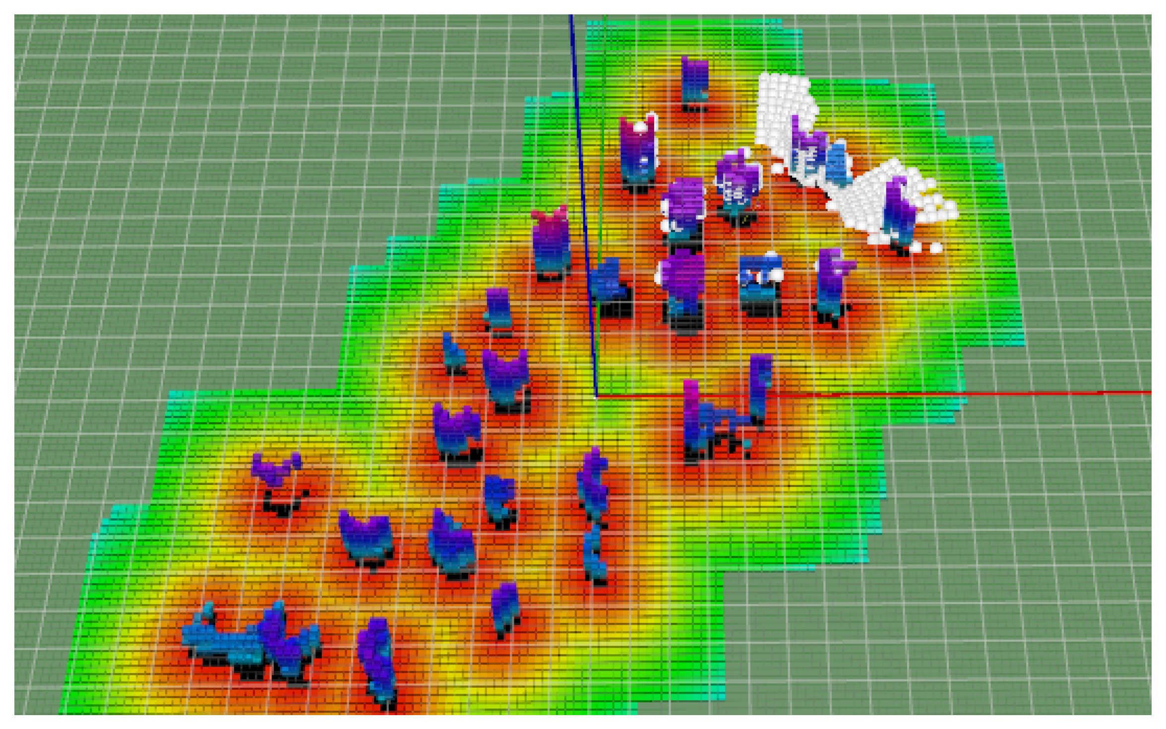
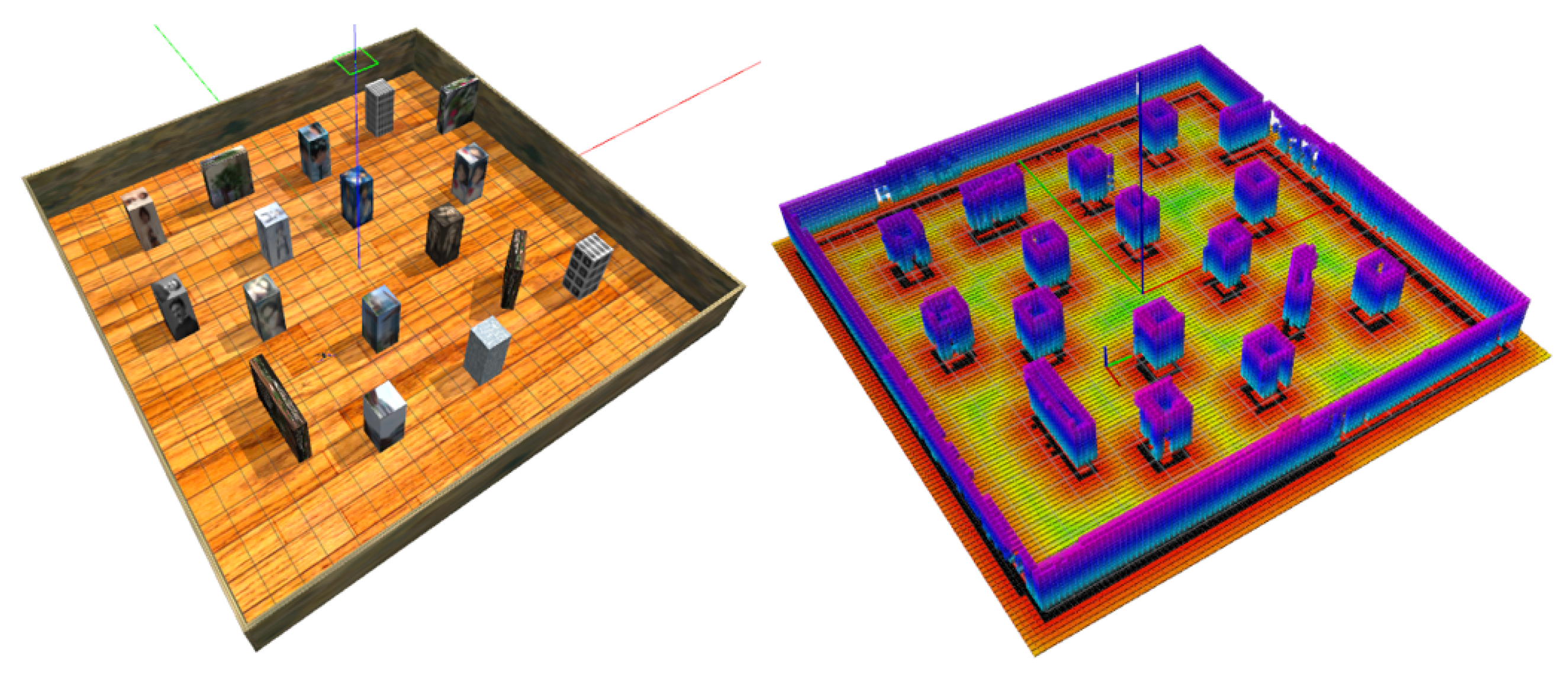
4.2. Mapping

A global-local mapping kit “glmapping” (https://github.com/HKPolyU-UAV/glmapping, accessed on 18 December 2021), which was developed by our group, was integrated into the simulator, as shown in Figure 8. This mapping kit is a 3D occupancy voxel map that was designed for MAV or mobile robot navigation applications. In the global map, the color (blue-purple) refers to the height of the obstacle, the ESFD map color (red-yellow-green) refers to the signed distance value, and the highlighted white spheres refer to the local map. Currently, most navigation strategies combine global planning and local planning algorithms. Global planning focuses on finding the lowest-cost path from the current position to the target destination. Furthermore, local planning is used to re-plan and optimize the trajectory to ensure smoothness and to avoid dynamic obstacles. This mapping kit processes perception information separately. The global map on a Cartesian coordinate system is a probability occupancy map, and the local map on a cylindrical coordinate system has excellent dynamic performance. The mapping kit also supports the projected two-dimensional (2D) occupancy grid map and the ESDF map output. The generated map can satisfy the requirements of both path-planning and environment visualization.

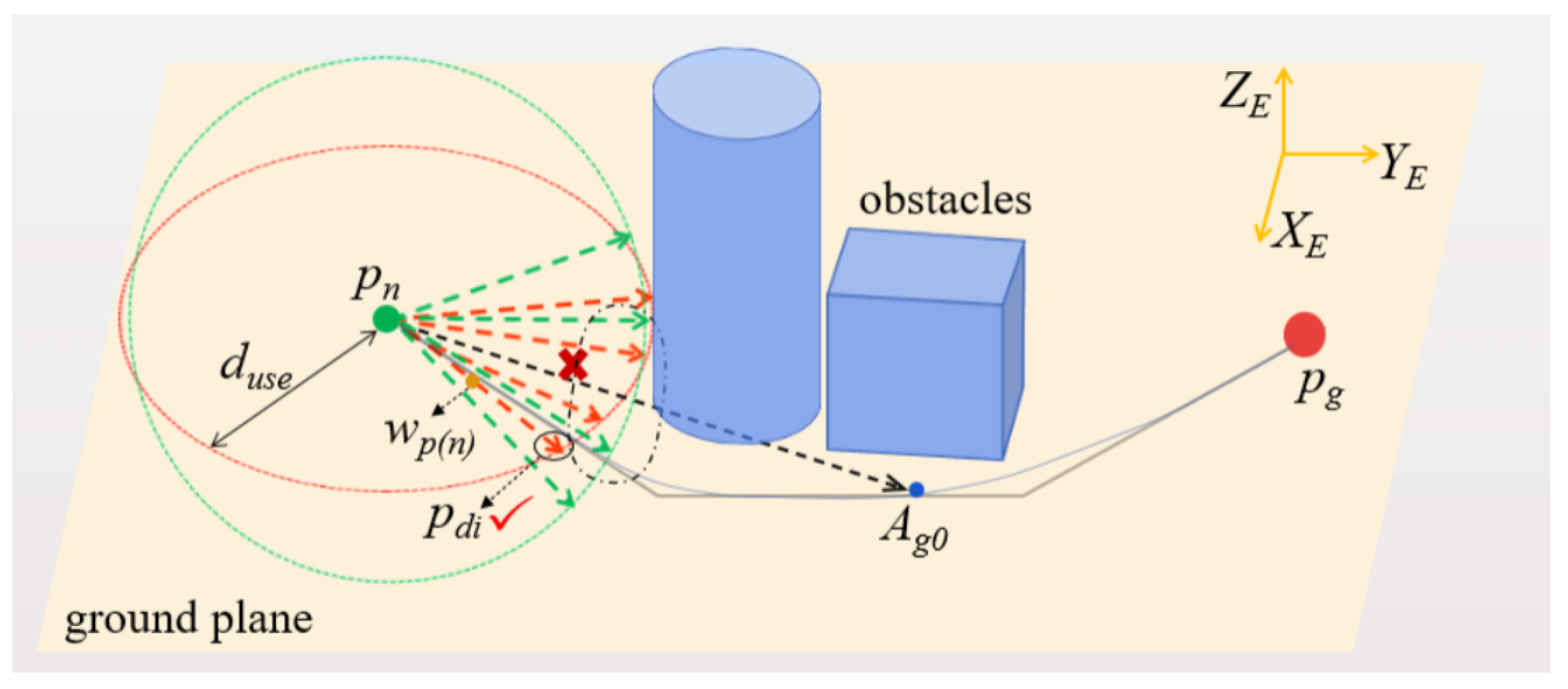
4.3. Path Planning and Obstacle Avoidance

The fuxi-Planner [27,35] was further integrated as the default path-planning kit. The planner is composed of a global path planner and a local planner and appears as an asynchronous parallel framework. The global planner works on a 2D global grid map to identify the shortest 2D path and to output the local goal of the local planner. The local planner works directly on the point cloud to avoid potential collisions with obstacles and to plan a kinematically feasible trajectory to the local goal. Algorithm 1 and Figure 9 illustrate the planning process. The local planner’s core component is a sample-based waypoint search method called the ’discrete angular search method’. The engagement of the global planner prevents the local planner from failing into the kidnap situation. The global planner uses the jump point search algorithm [36] to output a serial of waypoints, which represent the shortest path on the projected 2D grid map. The waypoints are then transformed and used as the control points to draw a Bézier curve. The local motion planner’s goal is to locate one sample point from the Bézier curve.

The initial search direction for the discrete angular search progress starts from $A_{g0}$, which consists of the horizontal and vertical direction angles from the drone’s position $p_n$ to the sample point. As shown in Figure 9, a group of line segments spread out from the initial search direction $A_{g0}$, and these line segments have a common start point $p_n$ and the same length $d_{use}$. $d_{use}$ is the point cloud distance threshold, the points whose distances from $p_n$ further than $d_{use}$ are not considered in the collision check. The two arrows of symmetry about $A_{g0}$ on the plane parallel to the ground plane are first checked to see if they collide with obstacles. If they will collide, the two lines in the vertical plane will be checked. These four lines have the same angle difference from $A_{g0}$. If the minimal distance between the line and the obstacles is smaller than the pre-assigned safety radius, it is treated as a collision. Figure 9 shows when the first round of the search has failed (arrows in the black dashed circle), another round with greater angle of difference is conducted until a collision-free direction, $\overrightarrow{p_n{p}_{di}}$, is found. Finally, the motion optimization problem is solved, taking point $w_{p\left(n\right)}$ as the endpoint constraint and generating the final motion primitives controlling the drone through $w_{p\left(n\right)}$ and respecting the kinodynamic limits. $w_{p\left(n\right)}$ is on $\overrightarrow{p_n{p}_{di}}$, and $|p_n{w}_{p\left(n\right)}|$ should satisfy the safety analysis in [35]. Although the global planner’s outer loop frequency is relatively low, the local planner’s inner loop still maintains a high update rate and can continuously command the UAV.

Algorithm 1 fuxi-Planner

1: while goal not reached: do 2:    Receive a global 3D voxel map $Pc{l}_m$, and its projecttion on the ground ($Map1$) as the 2D pixel map for path finding 3:    Cut off blank edge of $Map1$ and apply obstacle inflation on $Map1$, output $Map2$ 4:    Find the shortest $Path1$ to goal 5:    Calculate the optimal local goal by the Bezier curve 6: end while 7: while goal not reached: do 8:    Receive the local goal 9:    Find the next waypoint $N_k$ by heuristic angular search 10:    if $foundafeasiblewaypoint:$ then 11:      Run the minimum acceleration motion planner to get motion primitives 12:    else 13:      Run the backup plan for safety, then go to 5 14:    end if 15:    Send the motion primitives to the UAV flight controller 16: end while

5. Simulation Results and Performance Analysis

In this section, we report two experiments conducted to demonstrate the performance of the proposed simulator. In the first experiment, the vehicle was manually flown in the simulation world using the keyboard to verify the performance of the localization and mapping kits. In the second experiment, click-and-fly autonomous navigation was used.

The accuracy of the v-SLAM localization is presented by the absolute pose error (APE) of translation and rotation [37]. The definitions of APE is:

$${\mathit{E}}_{ape,n}={{\mathit{T}}_n^{gt}}^{-1}\mathit{S}{\mathit{T}}_n^{est},$$

(8)

where ${\mathit{T}}_n^{gt}$ is the transformation of the ground truth of frame n, ${\mathit{T}}_n^{est}$ is the transformation estimate of frame n, and $\mathit{S}$ is the least-squares estimation of transformation between the estimated trajectory ${\mathit{T}}_{1:m}^{est}$ and the ground truth trajectory ${\mathit{T}}_{1:m}^{gt}$ by Umeyama’s method [38]. The alignment transformation has six degrees of freedom ($\mathit{S}\in SE\left(3\right)$). In detail, the translation and rotation errors are defined by the root mean square error (RMSE) of APE, using:

$$\begin{array}{cc}\hfill {APE}_{trans}& =RMSE\left({\mathit{E}}_{ape,1:m}\right)\hfill \\ \hfill & =\sqrt{\frac{1}{m}\sum _{n=1}^m{∥trans\left({\mathit{E}}_{APE,n}\right)∥}^2}\hfill \end{array}$$

(9)

$$\begin{array}{cc}\hfill {APE}_{rot}& =RMSE\left({\mathit{E}}_{1:m}\right)\hfill \\ \hfill & =\sqrt{\frac{1}{m}\sum _{n=1}^m{∥rot\left({\mathit{E}}_{APE,n}\right)-{\mathit{I}}_{3x3}∥}^2}.\hfill \end{array}$$

(10)

The mapping kit will generate an reconstructed map. The agreement of this reconstructed map and the simulation world can also represent the accuracy of the localization kit and the overall performance of the mapping kit.

5.1. Manual Exploration

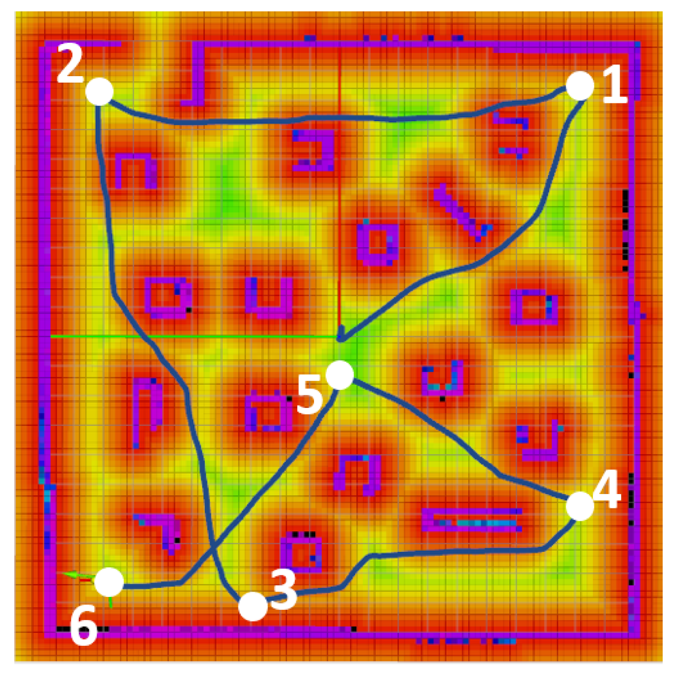
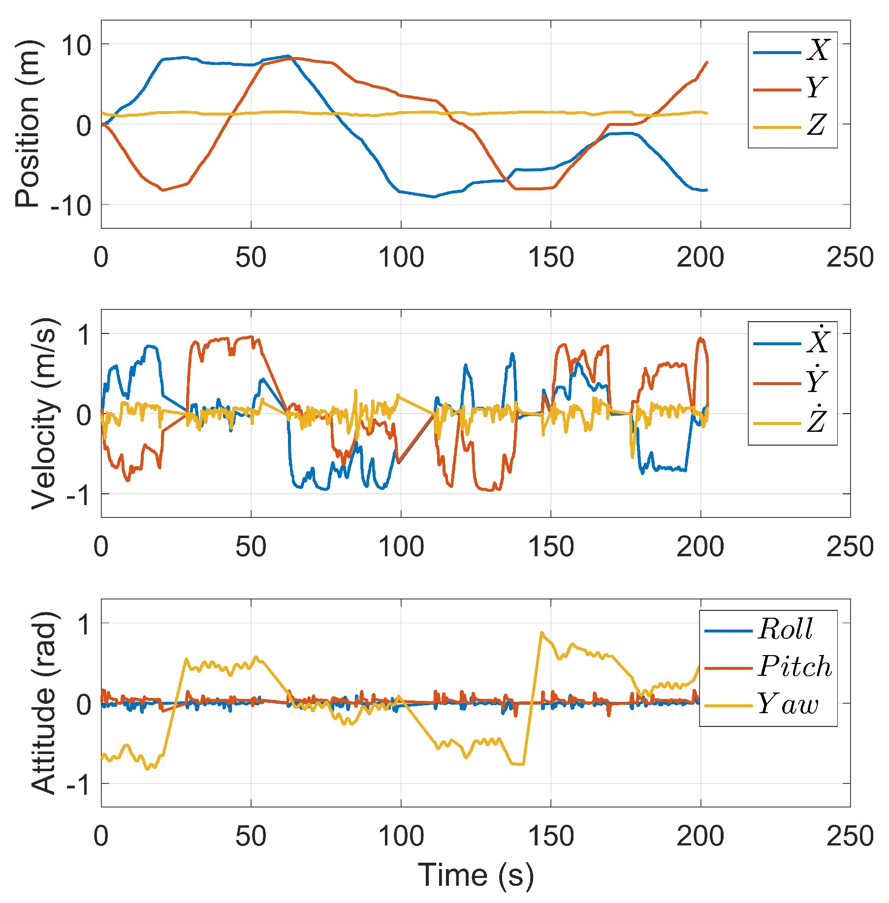
5.1.1. A 20 m × 20 m Room Environment

In this experiment, the localization and mapping kits were integrated. Using the first-person view from the color camera and the real-time reconstructed map view, the UAV was controlled to explore the 20 m × 20 m unknown environment. The exploration mission took 7 min and 24 s, and the UAV traveled 82 m in the simulation world.

The excellent agreement between the ground truth path and the estimated path of the localization kit is shown in Figure 10. A tool from Michael Grupp [37] was also used to evaluate the accuracy of the localization kit. The ${APE}_{trans}$ and ${APE}_{rot}$ of the trajectory was 0.3 m and 0.9 degree.

Images of the simulated world and the reconstructed map were captured from different viewpoints. Good agreement between them and the detail of the map can be observed in Figure 11 and Figure 12. The voxel size of the map was $0.2\times 0.2\times 0.2$ m.

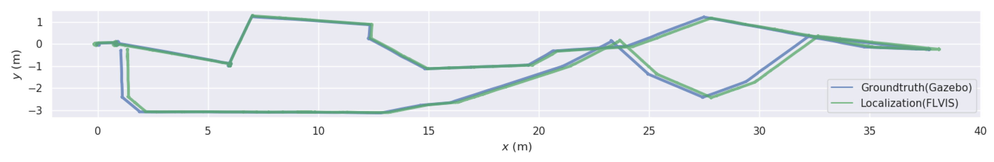
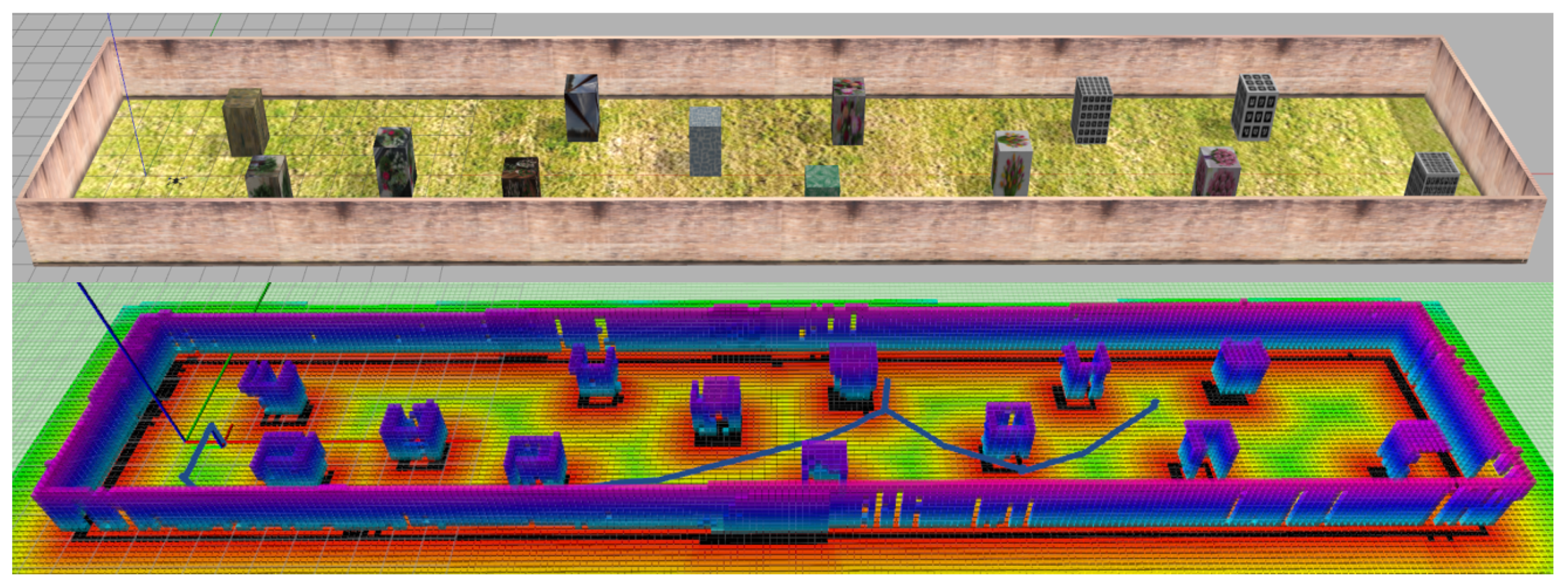
5.1.2. An 8 m × 40 m Corridor Environment

Another manual exploration experiment was carried out in an 8 m × 40 m unknown environment; this kind of environment setup represents the typical scenarios of flying in the jungle or a long corridor. Figure 13 shows the comparison of the ground truth and the estimated trajectory. The length of the trajectory was 100.4 m and the ${APE}_{trans}$ and ${APE}_{rot}$ of the trajectory were $0.3$ m and 0.9 degree, respectively. Figure 14 shows the good agreement of the simulation world and the reconstructed map.

5.2. Click-and-Fly Level Autonomy

In this case, the path-planning kit was further integrated into the simulation platform. Only the target destination was provided to the UAV on the map. Following this, the UAV planned a path to avoid the obstacles and to automatically fly to the target destination. As shown in Figure 15, six waypoints were set during the mission. The UAV perceived the environment and planned a path to automatically visit these waypoints in sequence. The UAV kept a safe distance from the nearest obstacle to avoid collision.

Figure 16 displays the position, velocity, and attitude plots of the simulation. The velocity was well controlled under the speed limit (1 m/s). Moreover, the position curves are fluent and pass all of the six goal points in a stable manner. The pitch and roll angles are small, suggesting that the vision localization kit had good performance.

5.3. The Processing Speed of Simulation

The navigation system was configured as follows. In the localization kit, the input image resolution was $640\times 360$; in the mapping kit, the voxel size was 0.2 m × 0.2 m × 0.2 m; and the map contained 181,500 ($110\times 110\times 15$) voxels. The simulation was verified on two different computers. The processing times are listed in

Table 1. Processing Time of the Navigation System and the Simulation Time Factor.

Kits		Computer 1	Computer 2
Localization (with out-loop closure)		28 ms	22 ms
Mapping	Global map	26 ms	18 ms
	Local map	4 ms	4 ms
	Projected ESDFs map	70 ms	64 ms
Planning	Global planning	90 ms	65 ms
	Local planning	20 ms	16 ms
Simulator	Average time factor	0.6	0.92

Note: Computer 1: i5-8250u CPU, 8 GB RAM, GeForce MX150 graphic card; Computer 2: i7-8550u CPU, 16 GB RAM, GeForce MX150 graphic card.

. The average time factor refers to the ratio of the actual time over the simulation time. A time factor value of 1 means that the simulation was run in real time.

5.4. Discussions

The main features of commonly used UAV simulators are listed in

Table 2. Features of Several UAV Simulation Platforms.

Features	E2ES	XTDrone [8]	AirSim [39]	FlightGoggles [40]
Rendering Engine	OpenGL	OpenGL	Unreal Engine	Unity
Dynamics	Gazebo	Gazebo	PhysX	User Define
Localization	Support	Support	Support	Support
Planning	Support	Support	Support	Support
Full Stack Solution	Support	Not Support	Not Support	Not Support
Multiple Vehicles	Not Support	Support	Support	Not Support

. The AirSim [39] and FlightGoggles [40] have more realistic visual effects, since they adopt game engines to render the scenes. The E2ES and XTDrone are based on the gazebo-PX4 toolchain, which means the algorithm can directly port to command the PX4 flight-control unit. Compared to other simulation frameworks, E2ES provides a full-stack solution. However, as this work focused on providing an out-of-box, end-to-end v-SLAM and navigation simulation, extended types of UAV models (airplanes, helicopters, etc.) and multi-vehicle simulation will be supported in the later versions.

6. Conclusions and Future Works

In this study, an end-to-end UAV simulation platform for SLAM, navigation research, and applications was introduced, including the detailed simulator setup and an out-of-box localization, mapping, and navigation system. The click-and-fly level autonomy navigation used by the simulator was also demonstrated. The flight results show that the simulator could provide a trustworthy data stream and versatile interfaces for the development of UAV autonomous function. We have offered all the kits for public access to promote further research and development of the autonomous UAV system based on this framework. Future work will focus on two aspects. One is to support more notable open-source navigation-related kits and, moreover, to design the benchmark scenario in the simulator to evaluate the performance of these kits. Another aspect is to expand the current simulator to encompass more perception sensors, more UAV models, and more challenging environments for a variety of potential tasks.

References

- Oleynikova, H.; Millane, A.; Taylor, Z.; Galceran, E.; Nieto, J.; Siegwart, R. Signed distance fields: A natural representation for both mapping and planning. In Proceedings of the RSS 2016 Workshop: Geometry and Beyond-Representations, Physics, and Scene Understanding for Robotics, Ann Arbor, MI, USA, 19 June 2016. [Google Scholar]
- Zhang, M.; Qin, H.; Lan, M.; Lin, J.; Wang, S.; Liu, K.; Lin, F.; Chen, B.M. A high fidelity simulator for a quadrotor uav using ros and gazebo. In Proceedings of the IECON 2015-41st Annual Conference of the IEEE Industrial Electronics Society, Yokohama, Japan, 9–12 November 2015; pp. 2846–2851. [Google Scholar]
- Alzugaray, I.; Teixeira, L.; Chli, M. Short-term UAV path-planning with monocular-inertial SLAM in the loop. In Proceedings of the 2017 IEEE International Conference on Robotics and Automation (ICRA), Singapore, 29 May–3 June 2017; pp. 2739–2746. [Google Scholar]
- Hartman, D.; Landis, K.; Mehrer, M.; Moreno, S.; Kim, J. dch33/Quad-Sim. Available online: https://github.com/dch33/Quad-Sim (accessed on 17 December 2021).
- Sun, J.; Li, B.; Wen, C.Y.; Chen, C.K. Design and implementation of a real-time hardware-in-the-loop testing platform for a dual-rotor tail-sitter unmanned aerial vehicle. Mechatronics 2018, 56, 1–15. [Google Scholar] [CrossRef]
- Furrer, F.; Burri, M.; Achtelik, M.; Siegwart, R. Robot Operating System (ROS): The Complete Reference; Chapter RotorS—A Modular Gazebo MAV Simulator Framework; Springer International Publishing: Cham, Switzerland, 2016; Volume 1, pp. 595–625. [Google Scholar] [CrossRef]
- Schmittle, M.; Lukina, A.; Vacek, L.; Das, J.; Buskirk, C.P.; Rees, S.; Sztipanovits, J.; Grosu, R.; Kumar, V. OpenUAV: A UAV testbed for the CPS and robotics community. In Proceedings of the ACM/IEEE 9th International Conference on Cyber-Physical Systems (ICCPS), Porto, Portugal, 11–13 April 2018; pp. 130–139. [Google Scholar]
- Xiao, K.; Tan, S.; Wang, G.; An, X.; Wang, X.; Wang, X. XTDrone: A Customizable Multi-rotor UAVs Simulation Platform. In Proceedings of the 2020 4th International Conference on Robotics and Automation Sciences (ICRAS), Wuhan, China, 12–14 June 2020; pp. 55–61. [Google Scholar] [CrossRef]
- Qian, J.; Chen, K.; Chen, Q.; Yang, Y.; Zhang, J.; Chen, S. Robust Visual-Lidar Simultaneous Localization and Mapping System for UAV. IEEE Geosci. Remote. Sens. Lett. 2021, 19, 1–5. [Google Scholar] [CrossRef]
- Sadeghzadeh-Nokhodberiz, N.; Can, A.; Stolkin, R.; Montazeri, A. Dynamics-Based Modified Fast Simultaneous Localization and Mapping for Unmanned Aerial Vehicles With Joint Inertial Sensor Bias and Drift Estimation. IEEE Access 2021, 9, 120247–120260. [Google Scholar] [CrossRef]
- Demim, F.; Nemra, A.; Mouali, O.; Hedir, M.; Rouigueb, A.; Hamerlain, M.; Bendoumi, M.A.; Bazoula, A. Simultaneous Localization and Mapping Algorithm based on 3D Laser for Unmanned Aerial Vehicle. In Proceedings of the 4th International Conference on Electrical Engineering and Control Applications, Constantine, Algeria, 17–19 December 2019; Bououden, S., Chadli, M., Ziani, S., Zelinka, I., Eds.; Springer: Singapore; pp. 1003–1020. [Google Scholar]
- Qin, T.; Li, P.; Shen, S. Vins-mono: A robust and versatile monocular visual-inertial state estimator. IEEE Trans. Robot. 2018, 34, 1004–1020. [Google Scholar] [CrossRef] [Green Version]
- Frost, D.; Prisacariu, V.; Murray, D. Recovering stable scale in monocular SLAM using object-supplemented bundle adjustment. IEEE Trans. Robot. 2018, 34, 736–747. [Google Scholar] [CrossRef]
- Pfrommer, B.; Daniilidis, K. TagSLAM: Robust SLAM with fiducial markers. arXiv 2019, arXiv:1910.00679. [Google Scholar]
- Mourikis, A.I.; Roumeliotis, S.I. A multi-state constraint Kalman filter for vision-aided inertial navigation. In Proceedings of the 2007 IEEE International Conference on Robotics and Automation, Rome, Italy, 10–14 April 2007; pp. 3565–3572. [Google Scholar]
- Bloesch, M.; Burri, M.; Omari, S.; Hutter, M.; Siegwart, R. Iterated extended Kalman filter based visual-inertial odometry using direct photometric feedback. Int. J. Robot. Res. 2017, 36, 1053–1072. [Google Scholar] [CrossRef] [Green Version]
- Leutenegger, S.; Lynen, S.; Bosse, M.; Siegwart, R.; Furgale, P. Keyframe-based visual–inertial odometry using nonlinear optimization. Int. J. Robot. Res. 2015, 34, 314–334. [Google Scholar] [CrossRef] [Green Version]
- Delmerico, J.; Scaramuzza, D. A benchmark comparison of monocular visual-inertial odometry algorithms for flying robots. In Proceedings of the IEEE International Conference on Robotics and Automation (ICRA), Brisbane, QLD, Australia, 21–25 May 2018; pp. 2502–2509. [Google Scholar]
- Gao, F.; Wu, W.; Gao, W.; Shen, S. Flying on point clouds: Online trajectory generation and autonomous navigation for quadrotors in cluttered environments. J. Field Robot. 2019, 36, 710–733. [Google Scholar] [CrossRef]
- Hornung, A.; Wurm, K.M.; Bennewitz, M.; Stachniss, C.; Burgard, W. OctoMap: An efficient probabilistic 3D mapping framework based on octrees. Auton. Robot. 2013, 34, 189–206. [Google Scholar] [CrossRef] [Green Version]
- Oleynikova, H.; Taylor, Z.; Fehr, M.; Siegwart, R.; Nieto, J. Voxblox: Incremental 3d euclidean signed distance fields for on-board mav planning. In Proceedings of the IEEE/RSJ International Conference on Intelligent Robots and Systems (IROS), Vancouver, BC, Canada, 24–28 September 2017; pp. 1366–1373. [Google Scholar]
- Han, L.; Gao, F.; Zhou, B.; Shen, S. Fiesta: Fast incremental euclidean distance fields for online motion planning of aerial robots. arXiv 2019, arXiv:1903.02144. [Google Scholar]
- LaValle, S.M. Rapidly-Exploring Random Trees: A New Tool for Path Planning; Technical Report; Computer Science Department, Iowa State University: Ames, IA, USA, 1998. [Google Scholar]
- Mellinger, D.; Kumar, V. Minimum snap trajectory generation and control for quadrotors. In Proceedings of the IEEE International Conference on Robotics and Automation (ICRA), Shanghai, China, 9–13 May 2011; pp. 2520–2525. [Google Scholar]
- Gao, F.; Lin, Y.; Shen, S. Gradient-based online safe trajectory generation for quadrotor flight in complex environments. In Proceedings of the IEEE/RSJ International Conference on Intelligent Robots and Systems (IROS), Vancouver, BC, Canada, 24–28 September 2017; pp. 3681–3688. [Google Scholar]
- Karaman, S.; Frazzoli, E. Sampling-based algorithms for optimal motion planning. Int. J. Robot. Res. 2011, 30, 846–894. [Google Scholar] [CrossRef]
- Chen, H.; Lu, P.; Xiao, C. Dynamic Obstacle Avoidance for UAVs Using a Fast Trajectory Planning Approach. In Proceedings of the IEEE International Conference on Robotics and Biomimetics (ROBIO), Dali, China, 6–8 December 2019; pp. 1459–1464. [Google Scholar]
- Quigley, M.; Conley, K.; Gerkey, B.; Faust, J.; Foote, T.; Leibs, J.; Wheeler, R.; Ng, A.Y. ROS: An open-source Robot Operating System. In Proceedings of the ICRA Workshop on Open Source Software, Kobe, Japan, 12–17 May 2009; Volume 3, p. 5. [Google Scholar]
- Koenig, N.; Howard, A. Design and use paradigms for gazebo, an open-source multi-robot simulator. In Proceedings of the IEEE/RSJ International Conference on Intelligent Robots and Systems (IROS), Sendai, Japan, 28 September–2 October 2004; Volume 3, pp. 2149–2154. [Google Scholar]
- Meier, L.; Honegger, D.; Pollefeys, M. PX4: A node-based multithreaded open source robotics framework for deeply embedded platforms. In Proceedings of the IEEE International Conference on Robotics and Automation (ICRA), Seattle, WA, USA, 26–30 May 2015; pp. 6235–6240. [Google Scholar]
- Lee, T.; Leok, M.; McClamroch, N.H. Geometric tracking control of a quadrotor UAV on SE (3). In Proceedings of the 49th IEEE Conference on Decision and Control (CDC), Atlanta, GA, USA, 15–17 December 2010; pp. 5420–5425. [Google Scholar]
- Mahony, R.; Kumar, V.; Corke, P. Multirotor Aerial Vehicles: Modeling, Estimation, and Control of Quadrotor. IEEE Robot. Autom. Mag. 2012, 19, 20–32. [Google Scholar] [CrossRef]
- Verling, S.; Weibel, B.; Boosfeld, M.; Alexis, K.; Burri, M.; Siegwart, R. Full Attitude Control of a VTOL tailsitter UAV. IEEE Int. Conf. Robot. Autom. 2016. [Google Scholar] [CrossRef] [Green Version]
- Chen, S.; Wen, C.Y.; Zou, Y.; Chen, W. Stereo Visual Inertial Pose Estimation Based on Feedforward-Feedback Loops. arXiv 2020, arXiv:2007.02250. [Google Scholar]
- Chen, H.; Lu, P. Computationally Efficient Obstacle Avoidance Trajectory Planner for UAVs Based on Heuristic Angular Search Method. In Proceedings of the IEEE/RSJ International Conference on Intelligent Robots and Systems (IROS), Las Vegas, NV, USA, 24 October–24 January 2021; pp. 5693–5699. [Google Scholar] [CrossRef]
- Harabor, D.; Grastien, A. Improving Jump Point Search. In Proceedings of the Twenty-Fourth International Conferenc on International Conference on Automated Planning and Scheduling (ICAPS’14), Portsmouth, NH, USA, 21–26 June 2014; pp. 128–135. [Google Scholar]
- Grupp, M. EVO: Python Package for the Evaluation of Odometry and SLAM. Available online: https://github.com/MichaelGrupp/evo (accessed on 17 December 2021).
- Umeyama, S. Least-squares estimation of transformation parameters between two point patterns. IEEE Trans. Pattern Anal. Mach. Intell. 1991, 13, 376–380. [Google Scholar] [CrossRef] [Green Version]
- Shah, S.; Dey, D.; Lovett, C.; Kapoor, A. AirSim: High-Fidelity Visual and Physical Simulation for Autonomous Vehicles; Field and Service Robotic; Springer International Publishing: Berlin/Heidelberg, Germany, 2018; pp. 621–635. [Google Scholar]
- Guerra, W.; Tal, E.; Murali, V.; Ryou, G.; Karaman, S. FlightGoggles: Photorealistic Sensor Simulation for Perception-driven Robotics using Photogrammetry and Virtual Reality. In Proceedings of the IEEE/RSJ International Conference on Intelligent Robots and Systems (IROS), Macau, China, 3–8 November 2019; pp. 6941–6948. [Google Scholar] [CrossRef] [Green Version]