Article

A Robust Reacting Flow Solver with Computational Diagnostics Based on OpenFOAM and Cantera

Department of Mechanical Engineering, University of Minnesota–Twin Cities, Minneapolis, MN 55455, USA
*
Author to whom correspondence should be addressed.
Current address: UM-SJTU Joint Institute, Shanghai Jiao Tong University, Shanghai 200240, China.
Aerospace 2022, 9(2), 102; https://doi.org/10.3390/aerospace9020102
Submission received: 4 January 2022 / Revised: 2 February 2022 / Accepted: 8 February 2022 / Published: 14 February 2022
(This article belongs to the Section Aeronautics)

Abstract

:
In this study, we developed a new reacting flow solver based on OpenFOAM (OF) and Cantera, with the capabilities of (i) dealing with detailed species transport and chemistry, (ii) integration using a well-balanced splitting scheme, and (iii) two advanced computational diagnostic methods. First of all, a flaw of the original OF chemistry model to deal with pressure-dependent reactions is fixed. This solver then couples Cantera with OF so that the robust chemistry reader, chemical reaction rate calculations, ordinary differential equations (ODEs) solver, and species transport properties handled by Cantera can be accessed by OF. In this way, two transport models (mixture-averaged and constant Lewis number models) are implemented in the coupled solver. Finally, both the Strang splitting scheme and a well-balanced splitting scheme are implemented in this solver. The newly added features are then assessed and validated via a series of auto-ignition tests, a perfectly stirred reactor, a 1D unstretched laminar premixed flame, a 2D counter-flow laminar diffusion flame, and a 3D turbulent partially premixed flame (Sandia Flame D). It is shown that the well-balanced property is crucial for splitting schemes to accurately capture the ignition and extinction events. To facilitate the understanding on combustion modes and complex chemistry in large scale simulations, two computational diagnostic methods (conservative chemical explosive mode analysis, CCEMA, and global pathway analysis, GPA) are subsequently implemented in the current framework and used to study Sandia Flame D for the first time. It is shown that these two diagnostic methods can extract the flame structure, combustion modes, and controlling global reaction pathways from the simulation data.

1. Introduction

High-fidelity reacting flow simulations are becoming more and more important nowadays with the increasing demand for designing clean and efficient energy conversion and propulsion technologies. The combustion processes in these technologies involve complex multi-component mixtures. As a result, robust reacting flow solvers with the capability to simulate the physical and chemical processes with detailed chemistry and transport properties for a large number of chemical species are fundamentally needed. In addition, it is well-known that the combustion processes in practical engines involve turbulence, and turbulence–chemistry interaction needs to be accurately understood [1]. Within OpenFOAM (OF) [2] computational fluid dynamics (CFD) platform, the reactingFoam solver contains multi-species finite-rate chemistry and thermodynamics, together with plenty of options for turbulence and turbulent combustion models, and is widely used in the combustion community [3,4].
However, as pointed out by a recent study [5], although the reactingFoam solver could give reliable results for highly turbulent reacting flows, it fails to predict laminar reacting flows accurately, especially for laminar flame speeds. The underlying reason is due to the simplified transport properties in OF, as pointed out in ref. [5]. In highly turbulent reacting flows, the multi-component molecular diffusion is dominated by turbulence mixing, and the effective unity Lewis number assumption used in OF is normally valid for temperature and the chemical species that dictate the heat release. However, in laminar reacting flows, molecular diffusion dominates, and the accurate evaluation of multi-component molecular transport properties (including viscosity, thermal conductivity, and mass diffusivity) becomes crucial to accurately predict low turbulent or laminar reacting flows. Conventionally in OF, the species viscosity is evaluated by Sutherland’s formula as a function of temperature. The thermal diffusivity and species mass diffusivities are then calculated via assumptions of unity Schmidt number and unity Lewis numbers, respectively. Implementing the more sophisticated and accurate multi-component [6] and mixture-averaged [7] transport models into OF is desirable. Moreover, one of the major concerns of applying these more accurate transport models into large scale reacting flow simulations is their high computational cost. As reported in ref. [8], constant but non-unity Lewis numbers for various species have very low computational cost and shown good consistency with the predicted results from the mixture-averaged transport model, thus it is a good compromise for large scale reacting flow simulations.
Although a few previous attempts of coupling more sophisticated transport models have been successful in [5,9], OF is still suffering from many other issues for reacting flow simulations. Firstly, although OF provides a chemistry reader to read reaction mechanisms in CHEMKIN format [10], some pressure-dependent fall-off reaction types (including Troe’s formula [11] and PLOG), which are widely used in chemical mechanisms, are not defined and supported in the OF chemistry models. Secondly, the stiff ordinary differential equation (ODE) solver in OF (i.e., Semi-implicit EULer EXtrapolation, SEULEX [12]) is reportedly unstable and unable to capture the low temperature combustion characteristics [5]. More specifically, Yang, Zhao, and Ge [5] found that in the Negative Temperature Coefficient (NTC) region, 14% relative errors are observed compared with the results by more robust stiff ODE solvers (e.g., the widely used variable-coefficient ODE solver in C, CVODE [13]). Finally, as reported by several studies [14,15], the most-widely used Strang splitting scheme [16] could have significant error because it cannot preserve the steady state exactly (i.e., not well-balanced). Even worse, OF uses a first-order accurate splitting scheme (which is not well-balanced), which, however, has never been discussed in the literature. The reactingFoam solver in OF without using well-balanced splitting schemes could lead to inaccurate flame extinction and re-ignition predictions [17].
Accordingly, the first objective of this paper is to tackle these issues and develop a robust and accurate reacting flow solver. To do so, the features of Cantera (an open-source suite of tools for problems involving chemical kinetics, thermodynamics, and transport processes) [18] reading chemical mechanisms and calculating reaction rates and transport properties are integrated into OF, enabling it to read mechanisms with more pressure-dependent fall-off reaction types. To introduce a more accurate ODE solver, the widely used CVODE is coupled, rendering accurate ODE solution for the chemical source terms in reacting flow simulations, especially for NTC region. In addition, the widely used second-order accurate Strang splitting scheme is added to replace the current first-order accurate solver. To minimize the splitting error when the transport flux terms and chemical source terms are at the same order of magnitude, a well-balanced splitting scheme [14] is also implemented in the current numerical framework.
Finally, high-fidelity reacting flow simulations with detailed chemistry generate large datasets [19]. It is difficult to extract useful information from such large datasets. To tackle this problem, we implemented two computational diagnostic methods into the current framework. Firstly, a conservative chemical explosive mode analysis (CCEMA) [20,21] is used to study the local chemical explosive and dissipative modes. However, CCEMA is not able to see how fuel/oxidizer is converted to the products (e.g., the global reaction pathway from fuel to products and all the intermediate steps). In this sense, a global pathway analysis (GPA) method [22,23] is used to complement CCEMA [19]. In GPA, the dominant global reaction pathways can be identified and we can understand the controlling conversion steps and elementary reactions.
In summary, the objective of this paper is to develop a robust reacting flow solver and associated analysis tools based on OF and Cantera, with the implementation of detailed chemistry and transport properties, a well-balanced splitting scheme and two advanced computational diagnostic tools. This framework could enable us to simulate and study the physio-chemical processes in combustion, with comprehensive diagnostics to understand the underlying physics and chemistry. The 0D and 1D ideal reactors, 1D and 2D laminar flames, and a 3D turbulent partially premixed jet flame are tested within this framework. The computational diagnostic methods (CCEMA and GPA) are used to analyze the 1D premixed flame and the 3D turbulent jet flame in this study.
The remaining of this paper is structured as follows. Section 2 introduces the numerical methodologies implemented and developed in this study. A variety of different flame configurations are simulated to demonstrate the accuracy and capabilities of the current framework in Section 3. Specifically, 0D auto-ignition cases are firstly simulated to prove the credibility of the chemistry reader and models. The 0D perfectly stirred reactor cases are then simulated to show the importance of well-balanced splitting schemes. In addition, 2D counter-flow diffusion flame simulations are conducted to test the transport models. Finally, 1D premixed flames and 3D partially turbulent flames are used to demonstrate the analysis of flames by the two diagnostic methods and their integration. Conclusions are then drawn in Section 4.

2. Methodology

2.1. Transport Models

The mass fraction transport equation for species k in a mixture with K species is given by
ρ Y k t + · ( ρ Y k u ) + · J k = r ˙ k ,
where Y k is mass fraction of the k-th species, ρ is mixture density and u is velocity. J k is molecular diffusion flux, which can be closed by different transport models. r ˙ k is the chemical source term. The enthalpy equation
ρ h t + · ( ρ h u ) + · q + τ : u = D p D t + Q ˙ ,
where q is the molecular heat flux, Q ˙ is the heat source terms including the chemical and radiative heat sources. D p D t is the the enthalpy changing rate due to compression and τ : u is the enthalpy changing rate due to viscous dissipation.
The molecular diffusion flux J k is calculated by the diffusion velocity V k
J k = ρ V k Y k .
Different transport models give different estimation on the diffusion velocity. In the multi-component diffusivity formulation, diffusion velocity is computed by
V k = ( j k K M j D k , j X j ) / X k M ¯ ,
where M k is the molecular weight of species k and M ¯ is the mean molecular weight of the mixture. X k is the molar concentration of species k, and D k , j is the binary diffusion coefficient of species k with respect to species j. Although this is considered to be the most accurate model, its complex and expensive calculation make it computationally prohibitive to be applied in 3D simulations of turbulent combustion with a lot of components [17]. Following the Fick’s Law, a simpler mixture-averaged model is typically used in combustion simulations, which calculates diffusion velocity by
V k = D k , m i x X k / X k ,
where D k , m i x is the mixture-averaged diffusion coefficient of species k and is computed by the binary coefficients D k , j :
D k , m i x = ( 1 Y k ) / j k K ( X j / D k , j ) .
It is noted there is no guarantee that the sum over mass diffusion of each species k = 1 K V k Y k is zero (in order to conserve mass) with the mixture-averaged diffusion velocity. Hence, an artificial correction is introduced by
V k c = V k j = 1 K V j Y j .
Even though this mixture-averaged transport model provides good approximation on mass diffusivity, it is still computationally expensive for 3D simulations of turbulent combustion (e.g., LES) [8]. Burali et al. [8] reported that using constant but non-unity Lewis numbers for LES provides acceptable accuracy, which calculates mass diffusivity based on species Lewis number and thermal diffusivity:
D k , m i x = α / L e k ,
where α is the thermal diffusivity and L e k is the Lewis number of species k. Since the species Lewis numbers are computed and provided a priori by counter-flow flame simulations based on mixture-averaged transport model, this constant but non-unity Lewis number model is computationally very efficient.
The three transport models mentioned above are implemented into OF, extending its capability for more accurate, as well as efficient simulations for both canonical flames and realistic combustors. In the mixture-averaged and multi-component models, the diffusion velocity is computed based on the molecular diffusivity coefficients obtained from Cantera.

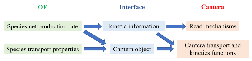
2.2. Chemistry Models and ODE Solvers

In OpenFOAM-6, two chemistry readers (i.e., FOAM chemistry reader and CHEMKIN reader) are provided for FOAM formatted and CHEMKIN formatted mechanisms, respectively. Simple elementary reactions, pressure independent third-body reactions and pressure-dependent fall-off reactions (e.g., Troe’s formula) can be read. Considering that CHEMKIN formatted mechanisms are the most widely used in the combustion community, one of the major weakness is that the current OF reaction types do not support “PLOG” pressure-dependent reaction type [24], which is adopted in more and more newly developed mechanisms (e.g., the AramcoMech [25]) and is supported in CHEMKIN-Pro and Cantera. The other major weaknesses of the current CHEMKIN reader in OF is its strict format requirement for the input files. Most of the current CHEMKIN mechanisms to be used in OF need some format modifications (e.g., lower case letters are not allowed), which is sometimes very tedious.
In order to address these weaknesses, Cantera is coupled into OF for chemical mechanisms reading, as shown in Figure 1, where the arrows from A to B indicate “A is obtained from B”. When OF needs to calculate species net production rate, it can either access the kinetic information obtained by the CT mechanism reader, or directly access the functions in the CT object (see Figure 1). In other words, two options are provided to deal with chemistry. The first option is to make the Cantera chemistry reader compatible with the current chemistry models in OF. To this end, after the Cantera mechanism reading, the species, thermodynamic and reaction data are embedded into OF. However, it should be pointed out that with this option, the PLOG reaction type is still not supported because OF lacks the necessary functions to handle this reaction type. The second option is to save the Cantera object (which contains all the thermodynamic and chemistry data) for later use in the chemistry models (e.g., estimating the reaction rates or specie production rates). In this way, any mechanism formats compatible in Cantera can also be used in OF. This option necessitates developing a new chemistry model class in OF (e.g., an addition to StandardChemistryModel in OF) to take advantage of the objects in Cantera. Thus, in this study, a Cantera Chemistry Model is developed and integrated into OF. As a result, all the functions for chemical kinetic calculations in the original standard chemistry model of OF are now accomplished by the functions from Cantera.
In addition, Yang, Zhao, and Ge [5] reported that the existing SEULEX stiff ODE solver in OF is not accurate to predict two-stage ignition and shows instability at different operating conditions. Except for the auto-ignition characteristics, ref. [26] also observed obvious discrepancy in terms of burning velocity calculations at near stoichiometric and rich conditions compared with the Cantera computed results. It is hence desirable to include a more robust stiff ODE solver into OF for chemistry integration. CVODES (i.e., CVODE with Sensitivity analysis capabilities) [27] in the SUNDIALS (Suite of Nonlinear and Differential/Algebraic equation Solvers) [28] library is widely adopted for stiff chemistry integration in combustion simulations, thus is integrated into OF via Cantera in this study.

2.3. Splitting Schemes

In OF reacting flow solvers, the solution of Equations (1) and (2) are achieved by a first-order accurate splitting scheme (named as ‘OF-splitting’ in this paper). To illustrate the splitting schemes in this section, the species and energy transport equations are rewritten as
d ϕ d t = T + R ,
where ϕ is the state variable vector, containing ρ Y k of all species and ρ h . T and R represent the transport term (including convection and diffusion) and chemistry source term, respectively. The OF-splitting scheme integrates R by solving the following ODE system with a stiff ODE solver and internal sub-cycling:
d ϕ d t = R ,
and obtains the first step solution ϕ * . OF then solves the equation
d ϕ d t = ϕ * ϕ 0 h + T ,
where h is the time step size, and ϕ 0 is the initial value. This way of splitting is only first-order accurate and not well-balanced (i.e., not preserving steady-state solutions) [29]. Other than OF-splitting, the most widely used splitting scheme in reacting flow simulations is the second-order accurate Strang splitting scheme [16], which symmetrically integrates Equation (9) by
d ϕ * d t = T ( ϕ * ) , ϕ * ( t n ) = ϕ n . d ϕ * * d t = R ( ϕ * * ) , ϕ * * ( t n ) = ϕ * ( t n + h / 2 ) . d ϕ * * * d t = T ( ϕ * * * ) , ϕ * * * ( t n + h / 2 ) = ϕ * * ( t n + h ) . ϕ ( t n + 1 ) = ϕ * * * ( t n + h ) .
It is widely reported that Strang splitting is not capable of accurately predicting flame extinction and ignition behavior when transport is at a similar time scale of reaction [14,15]. To address this issue, Lu et al. [15] and Wu, Ma, and Ihme [14] proposed well-balanced splitting schemes for those near-limit flames. The splitting scheme in Wu, Ma, and Ihme [14] (named as ‘Wu-splitting’ scheme hereafter) integrates transport and chemistry terms sequentially in such a fashion:
c n = T ( ϕ n ) . d ϕ * d t = R ( ϕ * ) c n , ϕ * ( t n ) = ϕ n . d ϕ * * d t = T ( ϕ * * ) + c n , ϕ * * ( t n + h / 2 ) = ϕ * ( t n + h ) . ϕ ( t n + 1 ) = ϕ * * ( t n + h ) .
As seen, due to the c n term introduced, the final integration step in Equation (13) is naturally well-balanced. This splitting scheme is implemented into the current numerical solver and used to solve Equations (1) and (2).

2.4. Conservative Chemical Explosive Mode Analysis (CCEMA)

We implemented a computational diagnostic method to identify the chemistry and flow contributions to combustion—the recently developed conservative CEMA (CCEMA) [21].
The original CEMA [30] was proposed to identify local chemistry state based on the eigen-analysis of local chemistry source term. The governing equations of a reacting flow system can be written as
D Φ D t = ω ( Φ ) + G ,
where Φ = [ c 1 , c 2 , . . . , T ] , representing the chemical species concentrations and temperature. G represents the transport terms. By taking the material derivative of ω with respect to time, the chemical Jacobian can be obtained by
D ω ( Φ ) D t = J · D Φ D t = J · [ ω ( Φ ) + G ] ,
where J = ω ( Φ ) Φ is the chemical Jacobian. As such, chemical modes are identified by the eigenvalues of J . Specifically, except for the conservation modes corresponding to element conservation and energy conservation, the other eigenvalues represents either explosive or dissipative modes of the local chemistry. The most positive real part of the eigenvalue λ e , if existing, implies that the local chemistry tends to explode eventually. The corresponding chemical mode associated with λ e is named as the chemical explosive mode (CEM). The contributions from each chemical species to CEM is quantified by the explosive index (EI), given by
EI = a e × b e a e × b e ,
where a e and b e are the right and left eigenvectors associated with λ e , respectively, and the symbol × indicates element-wise multiplication. CEMA is able to diagnose the flame and ignition front and detect the controlling chemical kinetics for the flame. Xu et al. [31] further extended CEMA by projecting the diffusion terms to the CEM:
D [ b e ω ( Φ ) ] D t = λ e b e · [ ω ( Φ ) + G d ] + ω ( Φ ) D b e D t = λ e · ( ϕ ω + ϕ d ) ,
where the term ω ( Φ ) D b e D t is ignored due to the fact that it has no effect on the ratio between ϕ ω and ϕ d (thus no effect on the following analysis) [32]. G d indicates the diffusion of Φ . With this way, it is then seen that the diffusion effect on CEM can be quantified by ϕ d , while the chemistry effect on CEM is ϕ ω . A parameter α is then defined as the ratio between ϕ d and ϕ ω and is used to detect the combustion regime, where α > 1 indicates diffusion assisted ignition, | α | < 1 indicates auto-ignition while α < 1 indicates diffusion inhibits the ignition process. As demonstrated by Wu et al. [21], the original CEMA needs special treatment to distinguish the energy conservation mode because temperature instead of internal energy is used in Φ . In addition, terms such as pressure work and compressibility contributions cannot be evaluated. Wu et al. [21] proposed to include momentum ( ρ u i ) and internal energy ( ρ e ) in the state variable vector Φ . In this way, the contributions of terms in the momentum and energy equations can be quantified. In detail, the contribution from compressibility G r and pressure work G p are considered by
D [ b e ω ( Φ ) ] D t = λ e b e · [ ω ( Φ ) + G d + G r + G p ] + ω ( Φ ) D b e D t = λ e · ( ϕ ω + ϕ d + ϕ r + ϕ p ) ,
where ϕ r = b e · G r and ϕ p = b e · G p . As pointed out by many previous CEMA studies [30,33,34], it is crucial to obtain a very accurate evaluation of chemical Jacobian matrix for CEMA analysis. The OF chemistry model, when dealing with pressure-dependent fall-off reactions, has a flaw, leading to inaccurate chemical Jacobian evaluation. Specifically, to evaluate the reaction rate of a Troe reaction, a Lindemann expression is firstly calculated based on a parameter F c e n t :
F c e n t = ( 1 a ) exp ( T T * * * ) + a exp ( T T * ) + exp ( T * * T ) ,
where a, T * * * , T * * and T * are specified reaction coefficients of the reaction (provided by chemical mechanisms). Note that the final parameter T * * are optional, meaning that the last term in Equation (19) should be zero if T * * is not specified in the reaction. However, OF regards the T**/T as a small number while exponential of a small number is not close to zero, which incurs large error and leads to inaccurate chemical Jacobian calculation. This flaw has been fixed in our new solver by directly setting the last term in Equation (19) to zero if T * * is not specified.

2.5. Global Pathway Analysis (GPA)

The Global Pathway Selection (GPS) algorithm was firstly proposed by Gao, Yang, and Sun [35] as a mechanism reduction tool and then extended to Global Pathway Analysis (GPA) [22,23,36] to find the dominant reaction pathways, as well as radical and elementary reactions controlling the phenomena of interest in a complex reacting system and the underlying connections among different species. In GPA, the most dominant reaction pathways based on element flux (i.e., global pathway (GP)) in a reacting system is firstly selected with the GPS algorithm. Then, the radical production and consumption, heat release and elementary reactions associated with the most dominant GP can be calculated at all spatial positions to study the chemical kinetic effects.
As the first step in GPA, an element flux graph is constructed, where each node in the graph represents one chemical species while the strengths of the edges connecting two nodes indicate the element (e.g., C, H, and O in hydrocarbon combustion processes) flux from one to another. The flux is calculated by
A e , i j = r a e , r , i j ,
where a e , r , i j is the contribution of the r-th reaction to the element flux of element e from the i-th species to the j-th species, which is computed by
a e , r , i j = max ( 0 , C e , r , i j R ˙ r ) ,
where R ˙ r is the net reaction rate of the r-th reaction. Zero value is used if R ˙ r is negative to ensure one direction flux from the i-th species to the j-th species. C e , r , i j is the element flux from the i-th species to the j-th species contributed by the r-th reaction, which is given by
C e , r , i j = n e , r , j n e , r , i n e , r v r , j v r , i < 0 ; 0 otherwise ,
where n e , r , i is the number of the e-th element transferred out from the i-th species in the r-th reaction, n e , r , j is the number of the e-th element transferred into the j-th species in the r-th reaction, n e , r is the number of the e-th element transferred in the r-th reaction, v r , i is the stoichiometric coefficient of the i-th species in the r-th reaction. The stoichiometric coefficient is positive for products and negative for reactants. In this way, C e , r , i j is zero when v r , j v r , i is positive, because the i-th and j-th species are in the same side in the reaction, indicating no element flux between them.
After the construction of element flux graph, a hub species is first defined by selecting the species that has the largest element flux through. The identification of GP after selecting the hub species is searching for the fastest path (i.e., the path with the largest geometric mean of the fluxes of links in the path) from the prescribed source species to the hub species and from the hub species to the sink species. The radical consumption and production associated with one certain GP R G P is then given by
R G P = D G P , e r G P Ω r ,
where D G P , e is the ratio of the e-th element number in the source species to the total number of the e-th element in all the initial species in the system. Ω r is the net radical production rate of the r-th reaction:
Ω r = ω r k δ k v r , k ,
where ω is the reaction rate of the r-th reaction. δ k is the 1 when the k-th species is OH, H, or O radical, and is 0 otherwise.
With the GPA method, we can identify the GPs that controls the carbon flux from fuel to products, and subsequently extract the significant conversion steps and the involved elementary reactions.
With all the methods aforementioned, we developed a reacting flow simulation and diagnostics platform based on OF and Cantera. Detailed transport and chemistry properties, new chemistry reader, stiff ODE solvers, splitting schemes, computational diagnostics tools are the special features of the current solver.

3. Results and Analysis

In this section, a variety of ideal reactors and laminar flames, and a turbulent partially premixed flame are simulated to test and show the capability of the solver. GPA and CCEMA are then conducted to understand the flame dynamics/modes and controlling chemical kinetics in the 1D premixed flame and 3D turbulent partially premixed flame.

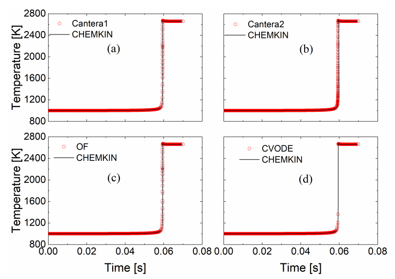
3.1. Zero-Dimensional Auto-Ignition: Chemistry Readers and Models, ODE Solvers

A 0D auto-ignition case is firstly conducted to validate the new chemistry reader and chemistry model from Cantera. GRI-Mech 3.0 mechanism [37] was used, and the SEULEX ODE solver was employed to integrate the chemistry except for the last case which applies the CVODES solver for comparison. The initial mixture is methane/air with unity equivalence ratio. The initial temperature is 1000 K and the pressure is constant at 1 bar. In Figure 2c, the original FOAM chemistry reader and FOAM standard chemistry model computed results are also plotted as references. Taking the CHEMKIN-II [10] results as the benchmark, as seen in Figure 2, digitally perfect agreements are achieved among different combinations of chemistry readers, chemistry models, and ODE solvers. The 0D auto-ignition calculations validate the current newly implemented chemistry reader (Figure 2b), chemistry model (Figure 2a), and ODE solver (Figure 2d). In all the following cases, CVODES stiff ODE solver, Cantera chemistry reader and Cantera chemistry model are used, except specified otherwise. The computational efficiency is found to be almost the same as Cantera.

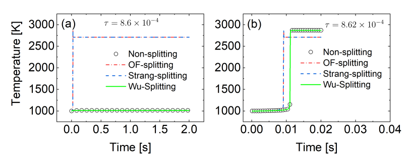
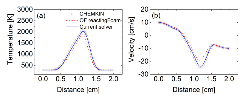
3.2. Zero-Dimensional Perfectly Stirred Reactor (PSR): Splitting Schemes

To show the importance of well-balanced splitting schemes, a PSR solver based on OF is first developed. Two hydrogen auto-ignition cases are then simulated, with the residence time τ = 8.6 × 10 4 (Figure 3a) and τ = 8.62 × 10 4 (Figure 3b) with a time step size h = τ / 100 . Note that the two residence times are chosen so that they are near the ignition and extinction limit, respectively. The hydrogen mechanism is from ref. [38], containing 10 species and 40 reactions (reverse reactions are counted separately). As seen in Figure 3, when τ = 8.6 × 10 4 where extinction is supposed to occur, the original OF splitting scheme and Strang-splitting scheme predict erroneous ignition. The well-balanced Wu-splitting scheme reproduces the extinction perfectly, compared with the benchmark case (without any splitting scheme and, hence, considered as the exact solution here). When τ = 8.62 × 10 4 where residence time is just long enough to allow ignition, the original OF splitting scheme and Strang-splitting scheme fail to capture the correct ignition delay. Compared with the non-splitting scheme, the Wu-splitting scheme reproduces the temperature profile and ignition delay in the reactor very well. The PSR tests with different splitting schemes in this section, thus, show that it is crucial to possess the well-balanced property for accurate ignition and extinction prediction in combustion simulations.

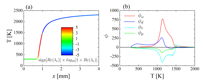
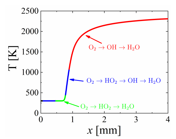
3.3. One-Dimensional Premixed Flame: CCEMA and GPA

To test the capability of the implemented CCEMA and GPA for reacting flow analysis, a 1D freely propagating premixed flame is tested and analyzed. The 1D premixed flame has an inlet of stoichiometric H2/air mixture at 300 K and 1 atm with a velocity of 2.4 m/s. A 9 species and 21 reaction H2 chemical mechanism [39] is used to model the H2 combustion. For scalars, the outlet boundary conditions are set to be zero gradient.
The temperature profile colored with the CEM eigenvalues is shown in Figure 4a. As has been seen, the CEM eigenvalues are able to clearly indicate the preheat zone, primary reaction zone, and final oxidation/burn-out zone. In addition, the projected diffusion ϕ d , compressibility ϕ r , and pressure work ϕ p terms in CEM are shown in Figure 4b. The diffusion term shows positive values in the preheat zone and its magnitude is larger than the chemical source term, indicating that before the reaction zone, diffusion assists the ignition by transporting fresh mixture from the preheat zone to the reaction zone and heat from reaction zone to the preheat zone. Compressibility and pressure work in this 1D flame are inhibiting ignition with negative projected values ( ϕ r and ϕ p ) in CEM.
GPA is then conducted to study the chemical kinetics for this 1D premixed flame. As shown in Figure 5, different dominant GPs are identified by GPA. It is noted that O2 (instead of H2 based on sensitivity analysis) is used as the source species here because it is well known that hydrogen flame is highly sensitive to O2 reactions with radicals [39]. From Figure 5, it is seen that the primary reaction zone and final oxidation/burn-out zone are dominated by the GP O2 → OH → H2O. In this GP, the elementary reaction is H + O2 = OH + O, which is reported in ref. [39] as one of the most important reactions involved H radical (based on sensitivity analysis). In the preheat zone, HO2 is firstly produced by the reaction O2 + H = HO2. As mentioned in ref. [39], this reaction is crucial for flame speed based on sensitivity analysis. Based on this analysis, we can see that GPA is able to identify the most dominant GPs at different flame zones and thus provide elementary reaction information to understand the key chemical kinetics at different flame zones, without conducting the computationally expensive sensitivity analysis.

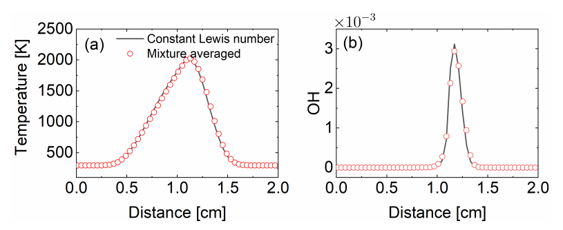
3.4. Two-Dimensional Counter-Flow Diffusion Flame: Molecular Transport Models

In this section, a 2D counter-flow diffusion flame is simulated to validate the various transport models implemented in the new reacting flow solver. With the mixture-averaged model, necessary molecular transport data (e.g., viscosity, thermal conductivity, and species mass diffusivity) is calculated in Cantera. The 2D counter-flow diffusion flame case is with pure methane stream and air stream flowing into the domain from two 1 cm × 1 cm inlets at a fixed velocity of 10 cm/s. The separation distance of two inlets is 2 cm. The grid size along the flow direction (x direction) is uniformly 0.2 mm. The faces in the y direction are set as outlets and their boundary conditions for scalars are zero gradient. The height and width of the domain were set to be 1 cm while the y direction is subdivided into 41 cells. GRI-Mech 3.0 mechanism [37] was used in this section. The same physical and chemical conditions, and chemical mechanism are also used in the CHEMKIN-Pro 1D counter-flow diffusion flame calculation to provide a reference solution due to the mixture averaged transport model and adaptive mesh used in CHEMKIN-Pro calculations.
In the original OF reacting flow solvers (e.g., reactingFoam), species viscosity coefficients are calculated by the Sutherland transport model, and then the thermal/mass diffusivity coefficients are evaluated by unity Schmidt/Lewis number assumption. As seen in Figure 6, the OF reactingFoam solver showed significant discrepancies from the CHEMKIN-Pro reference solution in terms of temperature (Figure 6a) and velocity profiles (Figure 6b). In contrast, as seen from Figure 6, good agreement was achieved between the CHEMKIN-Pro and the current solver using mixture-averaged transport model.
The constant Lewis number model is also implemented in this solver. As investigated in Burali et al. [8], the grid point with the maximum temperature is able to capture the flame features and thus species Lewis numbers at those points could well represent the ratio between thermal diffusivity and mass diffusivity in the flame. In this study, the counter-flow diffusion flame case is firstly simulated using the mixture-averaged transport model, where the species Lewis numbers at the maximum temperature grid points [8] are calculated and retrieved as inputs for the constant Lewis number flame calculation. The mass diffusivity coefficient in this new case is calculated with Equation (8). The predicted temperature (Figure 7a) and OH mass fraction profile (Figure 7b) with this constant non-unity Lewis number model is shown in Figure 7 and compared with the mixture-averaged transport model results. It is seen that the constant Lewis number model reproduces the temperature profile very well.

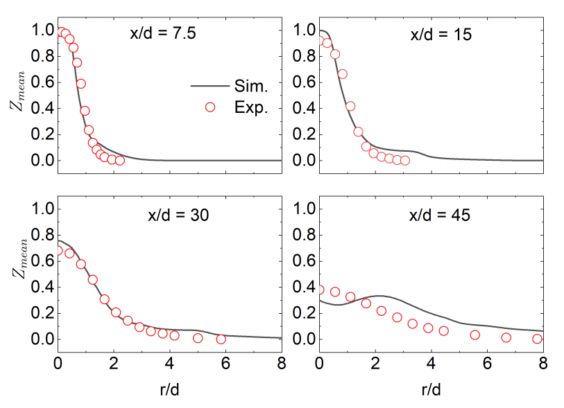
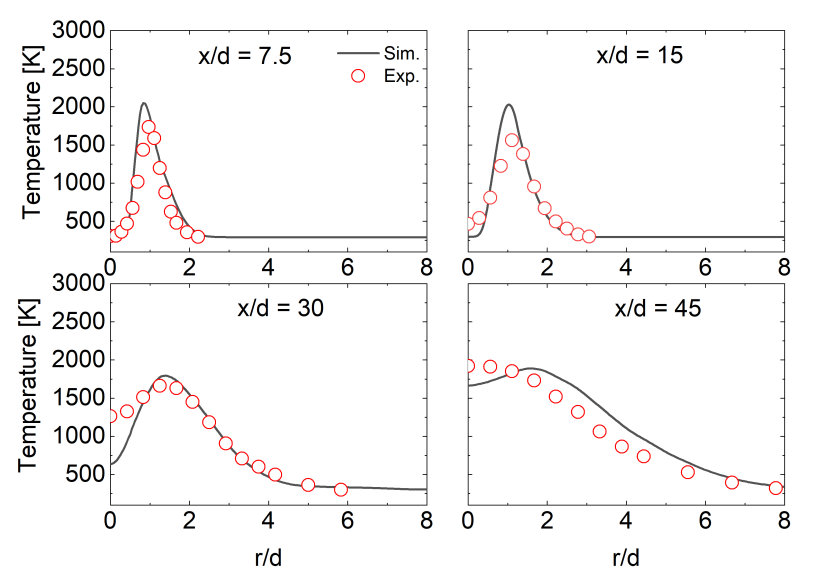
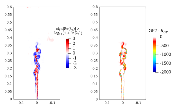
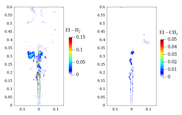
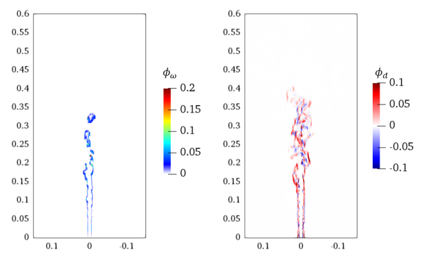
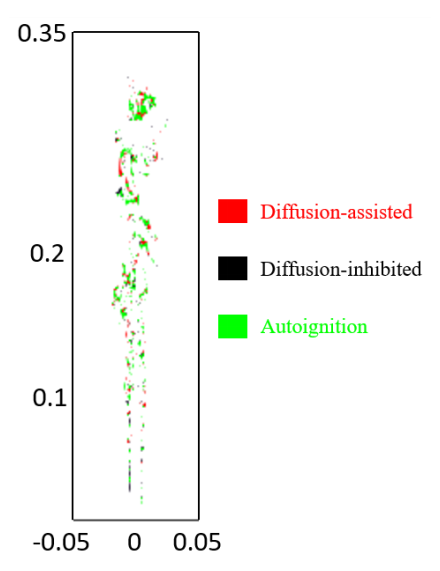
3.5. Three-Dimensional Turbulent Partially Premixed Flame: Integrated CCEMA and GPA

In this section, a large eddy simulation (LES) is conducted for a 3D turbulent partially premixed flame—Sandia Flame D [40]. Sandia Flame D documentation provides detailed experimental data and the flames are widely used to validate different CFD frameworks [41,42]. The flow conditions in Sandia Flame D is presented in Table 1.
Sandia Flame D has relatively simple geometry and fluid dynamics but complex turbulence–chemistry interaction, and, hence, is widely used as a benchmark case for combustion model/solver validations [1,43]. In this study, Sandia Flame D [40] is simulated with approximately 2.5 million grid points, where grid points in the jet and pilot regions are concentrated with the minimum grid size around 0.1 mm. In the axial direction, a cell size expansion ratio (the end cell size in this direction divided by the starting cell size in the same direction) of 2 is used. In the radial direction, the fuel jet and pilot regions are uniformly discretized, while the air co-flow region adopts a cell size expansion ratio of 3. Similar finest grid size (0.1 mm) is used in many other Sandia Flame D simulations [1,43] and, hence, is considered fine enough for the current LES study. The computational domain is 150D (where D is the jet diameter) in the axial direction and 60D in the radial direction. In LES, a series of filtered equations for mass, momentum, and species equations are solved. The Smagorinsky model [44] is used to close the subgrid-scale (SGS) turbulent flux terms in these filtered equations, which is also used in other Sandia Flame D studies [1,43,45]. A partially stirred reactor (PaSR) model [46] is used to close the unresolved chemical source term. GRI-Mech 3.0 mechanism [37] is used for the chemical kinetics. A turbulent inlet jet velocity boundary condition is used by adding perturbation (3% turbulence intensity) on the prescribed mean velocity profiles with a decaying turbulence inflow generator [47]. The outlet boundary conditions for all the scalars are zero gradient. The simulation starts with a cold flow, where the chemistry is frozen and uniform temperature (300 K), and velocity (49.6 m/s) is initialized in the domain. After two flow through times, the reaction starts and more than four flow through times are used to reach the statistically stationary state. Statistical mean values for temperature, mixture fraction and other major species are then collected over 6 flow through times. The maximum CFL number is set to 0.5 in the simulation.
The LES results with the newly developed solver are, firstly, compared to the experimental data. As shown in Figure 8, the predicted mixture fraction at four different axial positions agrees with the experimental data well (the maximum L 2 norm error for the four positions is less than 0.02). Temperature comparison is also shown in Figure 9 at four different axial positions and again, the experimental data are well predicted by the current simulations (the maximum L 2 norm error for the four positions is less than 10 K). At more downstream positions, both the mixture fraction and temperature show more obvious discrepancy compared with the measured data, which may be attributed to the accumulated error with the flow at downstream positions.
More importantly, we analyzed the LES results with the newly implemented CCEMA and GPA computational diagnostic tools. It is noted that the CCEMA and GPA results utilize the local chemistry and temperature for combustion modes and reaction pathway analysis. In LES, the filtered specie concentrations and temperature are used. The validity of local chemistry analysis for LES was discussed in refs. [20,21] and it showed that local chemistry analysis using filtered quantities could give reliable analysis for LES. The instantaneous temperature distribution on the Y plane is shown in Figure 10, together with the most dominant GPs at different regions. As shown, the most dominant GP for the main fuel jet burning region (axis 0.25–0.3 m) is majorly controlled by GP2 starting with CH4 + H = CH3 + H2. Further downstream, where temperature is below 1500 K, GP1 is the dominant pathway to convert fuel to products, indicating that in the low temperature region, the produced CH3 tends to generate C2H5 by reactions of H abstraction of C2H6 with C2H(s), O, OH, and CH3. R G P associated with GP2 is then calculated to show the radical production/consumption of this dominant GP, as shown in Figure 11. It is seen that GP2 is consuming radicals at the pilot-fuel shear layer and the main fuel jet burning region (axis 0.25–0.3 m). Compared with the eigenvalue plot of CCEMA in Figure 11, it is clearly seen that these radical consumption regions with GP2 coincide with the very negative eigenvalue region, implying that the dominant GP is rapidly consuming radicals and the mixture in this region is in dissipative mode and approaching equilibrium.
In Figure 12, the EI (as defined in Equation (16)) values of the important species (H2 and CH3) in GP1 and GP2 are presented to show the contribution of these species to the CEM. Figure 12 shows that H2 has maximum value of 0.15, indicating that it plays a significant role in contributing to the CEM. Note that the high H2 EI value region coincides with GP2 dominant regions (see Figure 10). It is thus seen that the integrated analysis with CCEMA and GPA is able to give us a comprehensive way to understand the contribution of species to the CEM and then the detailed reaction pathway information can be obtained by scrutinizing the conversion steps in the corresponding GP. CH3 is also shown in Figure 12 and it is found that contribution of CH3 to CEM is much less than H2. In addition, the follow-up reactions of H2 which generate H radicals, as indicated in GP2, are also significantly contributing to the CEM.
Finally, to further understand the combustion modes, the projections of reaction term ( ϕ ω ) and diffusion term ( ϕ d ) to the CEM are plotted in Figure 13. The projections of pressure work and compressibility terms to the CEM are trivial in this low-Mach flame, hence they are not shown in the figure. It is firstly seen that ϕ ω is significant at the pilot-fuel jet shear layer and the main fuel jet burning region (axis 0.25–0.3 m). As for ϕ d , both positive and negative values are shown, indicating that diffusion could both assist and inhibit combustion in the flame, depending on locations.
As introduced in Section 2.4, the ratio α between ϕ d and ϕ ω can be interpreted to distinguish different combustion modes, which is shown in Figure 14. It is seen that Sandia Flame D is a combination of auto-ignition-assisted and diffusion-assisted combustion in the shear layer. However, in the high temperature regions, diffusion is found to assist combustion at some locations but to inhibit the flame at some other locations.

4. Conclusions

The current work extends the capability of OpenFOAM (OF) dealing with chemical mechanisms with PLOG reaction types, as well as in integrating stiff chemistry with the widely used CVODES solver. A significant flaw for dealing with the Troe’s formula for pressure-dependent reactions is fixed in the OF. Then, two transport models (i.e., mixture averaged transport model and constant non-unity Lewis number model) are developed in OF by taking advantage of the transport properties calculated from Cantera. A second-order, accurate, well-balanced splitting scheme is implemented to robustly predict the near-limit combustion (i.e., near extinction/ignition). Finally, two computational diagnostics methods, global pathway analysis (GPA), and conservative chemical explosive mode analysis (CCEMA) are implemented to analyze combustion modes and controlling chemical kinetics in reacting flows, without conducting the computationally expensive sensitivity analysis. In addition, the flaws in the original OF for dealing with pressure-dependent fall-off reactions are fixed such that the chemical Jacobian evaluation can be sufficiently accurate for CCEMA.
With these newly-added features, a robust and accurate reacting flow solver with computational diagnostic tools is developed. The unsteady perfect stirred reactor (PSR) results show that the original first-order splitting scheme in OF and the popular second-order Strang splitting scheme could predict incorrect ignition/extinction behavior when transport is as significant as chemistry. In contrast, the newly-added well-balanced Wu-splitting scheme is able to predict the ignition/extinction correctly. In addition, the validation results in 0D auto-ignition, 1D premixed flame, 2D counter-flow diffusion flame, and 3D partially premixed turbulent flame showed good agreement compared with the CHEMKIN results. Detailed GPA and CCEMA analysis are then conducted for the 3D turbulent partially premixed flame (Sandia Flame D) for the first time. It is shown that the major fuel decomposition in Sandia Flame D is through the H radical with CH4. The combustion modes analysis indicates that Sandia Flame D is majorly controlled by auto-ignition combustion but accompanied by diffusion-assisted combustion. In the high temperature regions, diffusion is assisting combustion at some locations but inhibiting combustion at some other locations.

Author Contributions

Conceptualization, D.Z. and S.Y.; methodology, D.Z. and S.Y.; software, D.Z. and H.Z.; validation, D.Z.; formal analysis, D.Z. and H.Z.; investigation, D.Z.; resources, S.Y.; data curation, D.Z.; writing—original draft preparation, D.Z.; writing—review and editing, D.Z. and S.Y.; visualization, D.Z. and H.Z.; supervision, S.Y.; project administration, S.Y.; funding acquisition, S.Y. All authors have read and agreed to the published version of the manuscript.

Funding

S. Yang gratefully acknowledges the faculty start-up funding from the University of Minnesota—Twin Cities. H. Zhang gratefully acknowledges the support from the 3M Science and Technology Doctoral Fellowship, UMII MnDRIVE Graduate Assistantship Award, and Frontera Computational Science Fellowship.

Institutional Review Board Statement

Not applicable.

Informed Consent Statement

Not applicable.

Data Availability Statement

The data presented in this study are available on request from the corresponding author. The solver and CT-OF coupling interface are open source and can be found in https://github.com/UMN-CRFEL/OpenFOAM-Cantera (accessed on 31 January 2022).

Acknowledgments

The helpful discussion with Wantong Wu about CCEMA is greatly appreciated. The authors gratefully acknowledge the computational resources shared by the Minnesota Supercomputing Institute (MSI).

Conflicts of Interest

The authors declare no conflict of interest.

References

  1. Ihme, M.; Pitsch, H. Prediction of extinction and reignition in nonpremixed turbulent flames using a flamelet/progress variable model: 2. Application in LES of Sandia flames D and E. Combust. Flame 2008, 155, 90–107. [Google Scholar] [CrossRef]
  2. Jasak, H. OpenFOAM: Open source CFD in research and industry. Int. J. Nav. Archit. Ocean. Eng. 2009, 1, 89–94. [Google Scholar]
  3. Chen, Z.X.; Swaminathan, N.; Stöhr, M.; Meier, W. Interaction between self-excited oscillations and fuel–air mixing in a dual swirl combustor. Proc. Combust. Inst. 2019, 37, 2325–2333. [Google Scholar] [CrossRef] [Green Version]
  4. Huang, Z.; Zhao, M.; Xu, Y.; Li, G.; Zhang, H. Eulerian-Lagrangian modelling of detonative combustion in two-phase gas-droplet mixtures with OpenFOAM: Validations and verifications. Fuel 2021, 286, 119402. [Google Scholar] [CrossRef]
  5. Yang, Q.; Zhao, P.; Ge, H. reactingFoam-SCI: An open source CFD platform for reacting flow simulation. Comput. Fluids 2019, 190, 114–127. [Google Scholar] [CrossRef]
  6. Dixon-Lewis, G.N. Flame structure and flame reaction kinetics II. Transport phenomena in multicomponent systems. Proc. R. Soc. Lond. Ser. A Math. Phys. Sci. 1968, 307, 111–135. [Google Scholar]
  7. Bird, R.B.; Stewart, W.E.; Lightfoot, E.N. Transport Phenomena; John Wiley & Sons: Hoboken, NJ, USA, 2007. [Google Scholar]
  8. Burali, N.; Lapointe, S.; Bobbitt, B.; Blanquart, G.; Xuan, Y. Assessment of the constant non-unity Lewis number assumption in chemically-reacting flows. Combust. Theory Model. 2016, 20, 632–657. [Google Scholar] [CrossRef]
  9. Zhang, F.; Bonart, H.; Zirwes, T.; Habisreuther, P.; Bockhorn, H.; Zarzalis, N. Direct numerical simulation of chemically reacting flows with the public domain code OpenFOAM. In High Performance Computing in Science and Engineering’14; Springer: Berlin/Heidelberg, Germany, 2015; pp. 221–236. [Google Scholar]
  10. Kee, R.J.; Rupley, F.M.; Miller, J.A. Chemkin-II: A Fortran Chemical Kinetics Package for the Analysis of Gas-Phase Chemical Kinetics; Technical Report; Sandia National Lab. (SNL-CA): Livermore, CA, USA, 1989. [Google Scholar]
  11. Troe, J. Theory of Thermal Unimolecular Reactions in the Fall-off Range. I. Strong Collision Rate Constants. Berichte Bunsenges. FüR Phys. Chem. 1983, 87, 169–177. [Google Scholar] [CrossRef]
  12. Hairer, E. Solving Ordinary Differential Equations II: Stiff and Differential—Algebraic Problems, 1st ed.; Springer Series in Computational Mathematics Ser; Springer: Berlin/Heidelberg, Germany, 1991. [Google Scholar]
  13. Cohen, S.D.; Hindmarsh, A.C.; Dubois, P.F. CVODE, A Stiff/Nonstiff ODE Solver in C. Comput. Phys. 1996, 10, 138–143. [Google Scholar] [CrossRef] [Green Version]
  14. Wu, H.; Ma, P.C.; Ihme, M. Efficient time-stepping techniques for simulating turbulent reactive flows with stiff chemistry. Comput. Phys. Commun. 2019, 243, 81–96. [Google Scholar] [CrossRef]
  15. Lu, Z.; Zhou, H.; Li, S.; Ren, Z.; Lu, T.; Law, C.K. Analysis of operator splitting errors for near-limit flame simulations. J. Comput. Phys. 2017, 335, 578–591. [Google Scholar] [CrossRef]
  16. Strang, G. On the construction and comparison of difference schemes. SIAM J. Numer. Anal. 1968, 5, 506–517. [Google Scholar] [CrossRef]
  17. Gao, Y.; Liu, Y.; Ren, Z.; Lu, T. A dynamic adaptive method for hybrid integration of stiff chemistry. Combust. Flame 2015, 162, 287–295. [Google Scholar] [CrossRef]
  18. Goodwin, D.G.; Speth, R.L.; Moffat, H.K.; Weber, B.W. Cantera: An Object-oriented Software Toolkit for Chemical Kinetics, Thermodynamics, and Transport Processes. Version 2.4.0. 2018. Available online: https://www.cantera.org (accessed on 20 May 2019). [CrossRef]
  19. Zhou, D.; Zhang, H.; Yang, S. Computational Diagnostics for Reacting Flows with Global Pathway Analysis Aided by Chemical Explosive Mode Analysis. In Proceedings of the AIAA Scitech 2021 Forum, Nashville, TN, USA, 19–21 January 2021; p. 1368. [Google Scholar]
  20. Wu, B.; Zhao, X.; Xu, C.; Lu, T. Analysis of the chemical states of a bluff-body stabilized premixed flame near blowoff. In Proceedings of the AIAA Scitech 2019 Forum, San Diego, CA, USA, 7–11 January 2019; p. 0185. [Google Scholar]
  21. Wu, W.; Piao, Y.; Xie, Q.; Ren, Z. Flame diagnostics with a conservative representation of chemical explosive mode analysis. AIAA J. 2019, 57, 1355–1363. [Google Scholar] [CrossRef]
  22. Gao, X.; Gou, X.; Sun, W. Global Pathway Analysis: A hierarchical framework to understand complex chemical kinetics. Combust. Theory Model. 2018, 23, 1–23. [Google Scholar] [CrossRef]
  23. Yang, S.; Gao, X.; Sun, W. Global pathway analysis of the extinction and re-ignition of a turbulent non-premixed flame. In Proceedings of the 53rd AIAA/SAE/ASEE Joint Propulsion Conference, Atlanta, GA, USA, 10–12 July 2017; p. 4850. [Google Scholar]
  24. Gou, J.A.X.; Miller, W.S.; Ju, Y. 2011. Available online: http://engine.princeton.edu (accessed on 20 May 2019).
  25. Li, Y.; Zhou, C.W.; Somers, K.P.; Zhang, K.; Curran, H.J. The oxidation of 2-butene: A high pressure ignition delay, kinetic modeling study and reactivity comparison with isobutene and 1-butene. Proc. Combust. Inst. 2017, 36, 403–411. [Google Scholar] [CrossRef] [Green Version]
  26. Cloney, C.T.; Ripley, R.C.; Pegg, M.J.; Amyotte, P.R. Laminar burning velocity and structure of coal dust flames using a unity Lewis number CFD model. Combust. Flame 2018, 190, 87–102. [Google Scholar] [CrossRef]
  27. Serban, R.; Hindmarsh, A.C. CVODES: An ODE Solver with Sensitivity Analysis Capabilities; Technical report, Technical Report UCRL-JP-200039; Lawrence Livermore National Laboratory: Livermore, CA, USA, 2003. [Google Scholar]
  28. Hindmarsh, A.C.; Brown, P.N.; Grant, K.E.; Lee, S.L.; Serban, R.; Shumaker, D.E.; Woodward, C.S. SUNDIALS. ACM Trans. Math. Softw. 2005, 31, 363–396. [Google Scholar] [CrossRef]
  29. Speth, R.L.; Green, W.H.; MacNamara, S.; Strang, G. Balanced splitting and rebalanced splitting. SIAM J. Numer. Anal. 2013, 51, 3084–3105. [Google Scholar] [CrossRef]
  30. Lu, T.; Yoo, C.S.; Chen, J.; Law, C.K. Three-dimensional direct numerical simulation of a turbulent lifted hydrogen jet flame in heated coflow: A chemical explosive mode analysis. J. Fluid Mech. 2010, 652, 45–64. [Google Scholar] [CrossRef]
  31. Xu, C.; Park, J.W.; Yoo, C.S.; Chen, J.H.; Lu, T. Identification of premixed flame propagation modes using chemical explosive mode analysis. Proc. Combust. Inst. 2019, 37, 2407–2415. [Google Scholar] [CrossRef]
  32. Wu, K.; Zhang, P.; Yao, W.; Fan, X. Numerical investigation on flame stabilization in DLR hydrogen supersonic combustor with strut injection. Combust. Sci. Technol. 2017, 189, 2154–2179. [Google Scholar] [CrossRef] [Green Version]
  33. Shan, R.; Yoo, C.S.; Chen, J.H.; Lu, T. Computational diagnostics for n-heptane flames with chemical explosive mode analysis. Combust. Flame 2012, 159, 3119–3127. [Google Scholar] [CrossRef]
  34. Xu, C.; Poludnenko, A.Y.; Zhao, X.; Wang, H.; Lu, T. Structure of strongly turbulent premixed n-dodecane–air flames: Direct numerical simulations and chemical explosive mode analysis. Combust. Flame 2019, 209, 27–40. [Google Scholar] [CrossRef]
  35. Gao, X.; Yang, S.; Sun, W. A global pathway selection algorithm for the reduction of detailed chemical kinetic mechanisms. Combust. Flame 2016, 167, 238–247. [Google Scholar] [CrossRef]
  36. Zhou, D.; Yang, S. Soot-based Global Pathway Analysis: Soot formation and evolution at elevated pressures in co-flow diffusion flames. Combust. Flame 2021, 227, 255–270. [Google Scholar] [CrossRef]
  37. Smith, G.P.; Golden, D.M.; Frenklach, M.; Moriarty, N.W.; Eiteneer, B.; Goldenberg, M.; Bowman, C.T.; Hanson, R.K.; Song, S.; Gardiner, W.C., Jr.; et al. GRI-MECH 3.0. 1999. Available online: http://www.me.berkeley.edu/gri_mech/ (accessed on 20 May 2019).
  38. Ó Conaire, M.; Curran, H.J.; Simmie, J.M.; Pitz, W.J.; Westbrook, C.K. A comprehensive modeling study of hydrogen oxidation. Int. J. Chem. Kinet. 2004, 36, 603–622. [Google Scholar] [CrossRef]
  39. Li, J.; Zhao, Z.; Kazakov, A.; Dryer, F.L. An updated comprehensive kinetic model of hydrogen combustion. Int. J. Chem. Kinet. 2004, 36, 566–575. [Google Scholar] [CrossRef]
  40. Barlow, R.; Frank, J. Effects of turbulence on species mass fractions in methane/air jet flames. Symp. (Int.) Combust. 1998, 27, 1087–1095. [Google Scholar] [CrossRef]
  41. Pitsch, H.; Steiner, H. Large-eddy simulation of a turbulent piloted methane/air diffusion flame (Sandia flame D). Phys. Fluids 2000, 12, 2541–2554. [Google Scholar] [CrossRef]
  42. Jones, W.; Prasad, V. Large Eddy Simulation of the Sandia Flame Series (D–F) using the Eulerian stochastic field method. Combust. Flame 2010, 157, 1621–1636. [Google Scholar] [CrossRef]
  43. Yang, S.; Wang, X.; Huo, H.; Sun, W.; Yang, V. An efficient finite-rate chemistry model for a preconditioned compressible flow solver and its comparison with the flamelet/progress-variable model. Combust. Flame 2019, 210, 172–182. [Google Scholar] [CrossRef]
  44. Smagorinsky, J. General circulation experiments with the primitive equations: I. The basic experiment. Mon. Weather. Rev. 1963, 91, 99–164. [Google Scholar] [CrossRef]
  45. Yifan, D.; Zhixun, X.; Likun, M.; Zhenbing, L.; Huang, X.; Xiong, D. LES of the Sandia flame series DF using the Eulerian stochastic field method coupled with tabulated chemistry. Chin. J. Aeronaut. 2020, 33, 116–133. [Google Scholar]
  46. Golovitchev, V.I.; Nordin, N.; Jarnicki, R.; Chomiak, J. 3-D diesel spray simulations using a new detailed chemistry turbulent combustion model. SAE Trans. 2000, 109, 1391–1405. [Google Scholar]
  47. Mathey, F.; Cokljat, D.; Bertoglio, J.P.; Sergent, E. Assessment of the vortex method for large eddy simulation inlet conditions. Prog. Comput. Fluid Dyn. Int. J. 2006, 6, 58–67. [Google Scholar] [CrossRef]
Figure 1. Schematic of the integration between OF and Cantera.
Aerospace 09 00102 g001
Figure 2. Comparisons of temperature profiles of a 0D auto-ignition case between CHEMKIN-II [10] and (a) Cantera1: Cantera chemistry reader + Cantera chemistry model; (b) Cantera2: Cantera chemistry reader + OpenFOAM standard chemistry model; (c) OF: FOAM chemistry reader + OpenFOAM standard chemistry model; (d) CVODE: Cantera chemistry reader + Cantera chemistry model with CVODES.
Aerospace 09 00102 g002
Figure 3. Temperature profiles as a function of time in a perfect stirred reactor (PSR) with residence times of (a) 8.6 × 10 4 and (b) 8.62 × 10 4 , calculated with four different schemes. Symbols are the benchmark results, calculated without any splitting scheme.
Aerospace 09 00102 g003
Figure 4. (a) Temperature (T) profile in the 1D premixed flame as a function of the distance to the inlet (x), where temperature is colored by sign [ R e ( λ e ) ] × log 10 [ 1 + R e ( λ e ) ] . “sign” indicates the positive/negative sign. “Re” indicates the real part of a complex number. (b) The projected terms ( ϕ ) in CEM, as a function of temperature in the flame, where ϕ ω , ϕ d , ϕ r and ϕ p are the projections of reaction source term, diffusion term, compressibility term and pressure work term to the CEM, respectively.
Aerospace 09 00102 g004
Figure 5. Temperature (T) profile in the 1D premixed flame as a function of the distance to the inlet (x). The profile is colored by the most dominant global pathways (GPs).
Aerospace 09 00102 g005
Figure 6. Comparisons of (a) temperature and (b) axial velocity as functions of distance from the fuel side, among CHEMKIN-Pro, original OF reactingFoam solver, and the current solver. The results of CHEMKIN-Pro and current solver are calculated with mixture-averaged transport model.
Aerospace 09 00102 g006
Figure 7. (a) Temperature and (b) OH mass fraction profiles as functions of distance to the fuel inlet, calculated with the mixture-averaged transport model and constant non-unity Lewis number model, respectively.
Aerospace 09 00102 g007
Figure 8. Radial mean mixture fraction distribution in Sandia Flame D at x / d = 7.5 , x / d = 15 , x / d = 30 and x / d = 45 . Symbols are experimental data, while lines are simulation data.
Aerospace 09 00102 g008
Figure 9. Radial mean temperature distribution in Sandia Flame D at x / d = 7.5 , x / d = 15 , x / d = 30 and x / d = 45 . Symbols are experimental data, while lines are simulation data.
Aerospace 09 00102 g009
Figure 10. Instantaneous temperature distribution in Sandia Flame D on the x–z plane. Axial and radial coordinates are in meter. GP1: CH4 →CH3→CH2(S) →C2H5→C2H6→H2O. GP2: CH4→H2→ H → H2O. GP3: CH4→CH3→H2→ H →H2O. GP4: CH4→C2H4→C2H5→CH3→CH2(S) → CH →HCCO→ CO → CO2.
Aerospace 09 00102 g010
Figure 11. Instantaneous distributions of sign [ R e ( λ e ) ] × log 10 [ 1 + R e ( λ e ) ] (refer to Figure 4 for the meanings of the symbols), R GP for GP2: CH4→H2→ H → H2O, on the x–z plane in the flame. Axial and radial coordinates are in meter.
Aerospace 09 00102 g011
Figure 12. Instantaneous distributions of EI in Sandia Flame D for H2 and CH3 on the x–z plane. Axial and radial coordinates are in meter.
Aerospace 09 00102 g012
Figure 13. Instantaneous distributions of ϕ ω and ϕ d in Sandia Flame D on the x–z plane. Axial and radial coordinates are in meter.
Aerospace 09 00102 g013
Figure 14. Combustion modes in the Sandia Flame D. Red color corresponds to diffusion-assisted combustion, black color corresponds to diffusion-inhibited combustion, green color corresponds to auto-ignition dominant combustion. Axial and radial coordinates are in meter.
Aerospace 09 00102 g014
Table 1. Flow conditions in Sandia Flame D.
Fuel JetPiloted FlameCo-Flow
Composition25% CH4/75% air
(by volume)
CH4/air equilibrium
mixture ( ϕ = 0.77 )
Air
Inner diameter
(mm)
7.27.718.9
Outer diameter
(mm)
7.718.2N.A.
Bulk velocity
(m/s)
49.611.40.9
Temperature
(K)
2941880291
Publisher’s Note: MDPI stays neutral with regard to jurisdictional claims in published maps and institutional affiliations.

