Article

An Onboard Adaptive Model for Aero-Engine Performance Fast Estimation

School of Energy and Power Engineer, Beihang University, Beijing 100191, China
*
Author to whom correspondence should be addressed.
Aerospace 2022, 9(12), 845; https://doi.org/10.3390/aerospace9120845
Submission received: 14 November 2022 / Revised: 11 December 2022 / Accepted: 16 December 2022 / Published: 18 December 2022
(This article belongs to the Section Aeronautics)

Abstract

:
The onboard adaptive model is essential to the model-based control and diagnosis of the engine. However, current methods, such as the Kalman-based and the data-driven ones, cannot meet the demands of performance estimation well. Their self-tuning processes lead to a long period of model mismatch and, thus, degrade the quality of control and diagnosis, even causing engine failures. To overcome this disadvantage, a novel onboard adaptive model with fast estimation capability is proposed. The proposed method employs a component level model as the benchmark and introduces some scaling factors as the model tuners. These tuners are derived from the measurements and defined to quantify the characteristic deviations of the engine components at a certain operating condition. An algorithm with memory function is introduced to store the correlations between the tuners and the operating condition and, thus, predict these tuners according to the operating condition of inputs. By feeding the predicted tuners to the benchmark model, the engine performance can be estimated rapidly. Simulations are implemented to demonstrate the effectiveness of the proposed model. The results show that it has not only a high estimation accuracy at steady operating states, but also a short dynamic response time and the memory ability to avoid repeated self-tuning processes when the operating state of the engine varies.

1. Introduction

With the development of computer science, some advanced techniques, such as model predictive control [1], performance seeking control [2], direct thrust control [3], and model-based fault diagnosis [4], are emerging in the field of engine control in recent years. These techniques all require an onboard model to provide either measurable or unmeasurable parameters of the engine for control, monitoring, and diagnostics [5,6]. However, the engine inevitably suffers various physical faults (e.g., foreign object damage, blade erosion and corrosion, worn seals, excess clearances) during its service life. These faults lead to performance deterioration and, thus, mismatch between the onboard model and the engine [7,8]. Maintenance and installation would also cause a slight performance difference between individual engines of the same type [9,10]. These facts press the onboard model to have the self-tuning capability to eliminate the deviation. In addition, when the degradation degree or the operating state of the engine varies, a new self-tuning process is necessary to accommodate the changed deviation [11]. A slow estimation process can lead to a longtime mismatch and, thus, degrade the quality of control, monitoring, and diagnosis, even causing engine failures in severe scenarios. Therefore, establishing an onboard model with self-tuning and fast estimation capability is a key task in these above techniques.
To acquire the self-tuning capability, Luppold firstly employed a Kalman filter, which is implemented with a recursive algorithm and can estimate both system states and unmeasurable parameters in real-time, to provide a set of tuners that would adapt a piecewise state variable model to output a better match with the actual performance [12]. The tuners are derived by the residuals between the model and the measurements and consist of health parameters such as efficiencies and flow parameters [13,14]. Besides that, Panov proposed a Kalman-based performance tracking tool, in which the tuners generated by the filter were fed to a dynamic real-time model to match the degraded measurements [15]. Since the Kalman filter is an estimator applied to linear systems, the modeling error of the onboard model has a corruptive effect on the estimation results [16]. To address this problem, Volponi added an empirical neural network module, and Pang proposed an improved incremental linearized Kalman filter [17,18]. On the other hand, non-linear Kalman filters, such as the extended Kalman filter [19,20] and unscented Kalman filter [21,22], were introduced to construct a nonlinear onboard adaptive model due to a better estimation accuracy than the linear one. Burnell utilized the extended Kalman filter to establish an adaptive component level model and realized the nonlinear model predictive control based on the model [23]. Dewallef applied the unscented Kalman filter to monitor performance by estimating health parameters [24]. Yang compared the estimation results of these Kalman filters and concluded that the constant gain extended Kalman filter can achieve a better balance in accuracy and computation time [25].
However, the usage of nonlinear Kalman filters brings a heavy computation burden. To improve the real-time property, data-driven methods were proposed [26]. By establishing the mapping relationship between measurable output parameters and unmeasurable parameters offline, these methods can finish parameter estimation in a short period of computing time. Wang adopted a BP neural network to train the mapping relationship between the measured output biases and unmeasured ones so that the outputs of the onboard model were adapted to those of the real engine [27]. Wang constructed the mapping relationship between some measurable parameters and three deterioration condition parameters, based on a multi-input and multi-output recursive reduced least squares support vector regression algorithm, to realize the self-tuning capability of a turbo-shaft engine onboard model under the degraded condition [28]. Nevertheless, the drawback of the data-driven methods is that ensuring the model’s accuracy needs a lot of effective data [29]. In addition, the generalization ability of the algorithms used should be considered [30].
Although the Kalman-based methods and the data-driven methods have achieved satisfactory results in adaptive estimation, the capability of fast estimation is still an aspect that needs attention and a solution. In fact, the Kalman-based methods employ a multi-step iterative process to obtain optimal estimation results. The iterative process often spends several seconds to complete it. And the data-driven methods are influenced by the dynamic response of measurable output parameters, especially those measured by temperature sensors, which makes the results also have a dynamic response process of about 9 s [28]. As a consequence, the applications of the Kalman-based methods and the data-driven methods to model-based control and diagnosis are somewhat restricted.
Aiming at the defect of existing methods in fast estimation capability, a novel onboard adaptive model is proposed in this paper. The main contributions are as follows: (1) To speed up performance estimation, a novel modeling method is developed, which can eliminate the repetitive and long-time model mismatch. (2) A model tuner with quick availability is adopted in the model, which helps to assess the characteristic deviations of components rapidly. (3) An algorithm with memory function is employed to predict the tuners and, thus, shorten the time of self-tuning.
The remainder of this paper is organized as follows: Section 2 details the methodology of the proposed onboard adaptive model. Section 3 shows and discusses the simulation results to demonstrate the effectiveness of the model. Finally, Section 4 concludes this paper.

2. Methodology

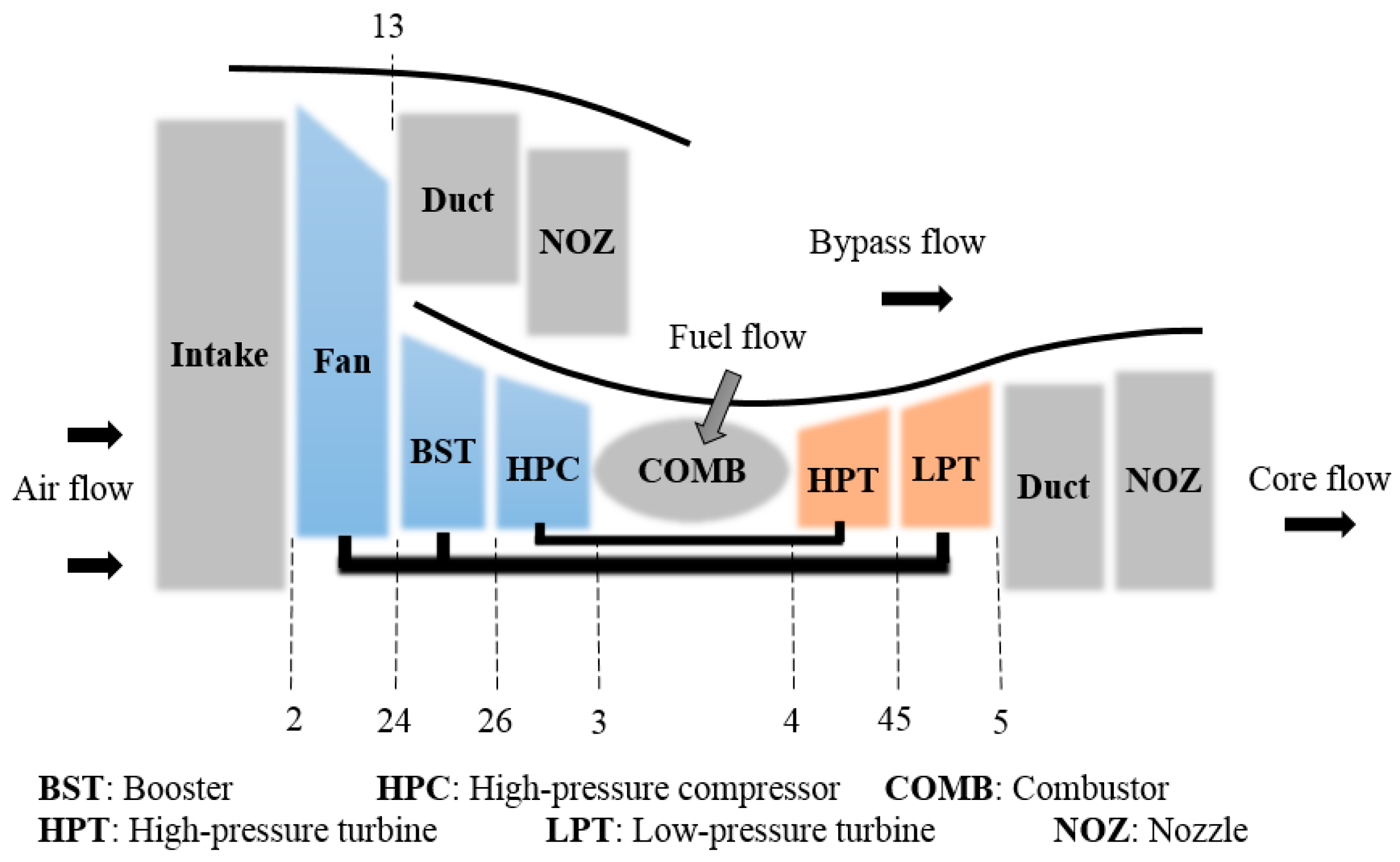
Without loss of generality, a typical civil high-bypass twin-shaft turbofan engine, which belongs to the General Electric CF6 series, is selected as the research object. The construction of this engine is shown in Figure 1, with components of intake, fan, booster, high-pressure compressor (HPC), combustor, high-pressure turbine (HPT), low-pressure turbine (LPT), duct and nozzle of bypass, and core. In addition, the engine has the following performance parameters at the design point: the thrust is 254.6 kN, the pressure ratio is 29.6, the fuel mass flow rate is 2.5236 kg/s, the high-pressure rotor speed is 10,270 rpm, and the low-pressure rotor speed is 3390 rpm.
The component level model of this turbofan engine is implemented using the Simulink Toolbox for the Modeling and Analysis of Thermodynamics Systems (T-MATS), which is an open-source modeling package on behalf of NASA [31]. The modeling procedures are summarized as follows: firstly, each component is modeled based on aero-thermodynamics principles. Then, considering the cooperation equations, which include the flow continuity equations, pressure balance equations, and power balance equations or rotor dynamics equations, the cooperation relationship among the component models is established. Finally, using the Newton–Raphson method to solve the formulated nonlinear equations, the measurable performance parameters, such as the rotor speeds, pressures, and temperatures in the flow path, and the unmeasurable parameters, such as thrust, can be derived. All the engine performance maps and relevant data are acquired from the gas turbine simulation program (GSP) [32].
The constructed model can be expressed with a system of non-linear differential equations in state space:
x ˙ = f ( x , u , v , ζ ) y = g ( x , u , v , ζ )
where x is the state vector, u is the input vector, v is the flight condition vector, ζ is the characteristic vector, and y is the output vector. All the vectors are column vectors, and the same are below, unless otherwise specified.
The state vector x contains the low-pressure rotor speed n l and the high-pressure rotor speed n h : x = [ n l , n h ] T . The flight condition vector v is composed of altitude H and Mach number Ma: v = [ H , M a ] T . The output vector y comprises measurable parameters y m and unmeasurable parameters y n : y = [ y m , y n ] T .
The input vector u = [ m ˙ f , α V G V , α B O V ] T consists of the following control variables: m ˙ f —fuel flow, α V G V —variable guide vane angle, and α B O V —bleed/blow-off valve angle. Together with the flight condition vector, it constitutes the engine’s operating condition. In fact, the engine’s operation is inseparable from the control system. For a closed-loop system containing the engine and the control system, the input vector is selected as the command of power level angle (PLA) for convenience: u = P L A . Correspondingly, Equation (1) describes the equations of the closed-loop system. It is worth mentioning that, in the closed-loop system, the PLA can still be translated to the engine’s control variables through the control system.
The characteristic vector ζ contains the characteristics of each component. Taking the HPC as an example, its characteristics include corrected mass flow, efficiency, pressure ratio, and corrected speed. When the components’ characteristics are at their nominal value, the component level model is a benchmark model. However, the characteristics would deviate from their nominal value and, thus, cause a mismatch between the benchmark model and the actual engine, when the engine is in deterioration. Therefore, for the component level model, obtaining the actual characteristics accurately and quickly is the key to its performance estimation capability.

2.1. Actual Characteristics Calculation

It seems like an inverse mathematical problem of Equation (1) to calculate the components’ actual characteristics according to the measurements. The known information is the operating condition and the measurable parameters, which contain the input vector u , the flight condition vector v , the state vector x , and the pressure and temperature of some stations, whereas the actual characteristics are unknown. To compute the characteristics of all components, a single point adaptation method is developed from existing approaches [33,34,35,36] and described as follows. It should be noted that data handling is required to eliminate the abnormal data before applying the method.
Let the known information be defined as the known parameters z and the unknown components’ characteristics defined as the to-be-adapted parameters ζ ¯ . It should be noted that some characteristics can be obtained directly from z , such as the corrected speed of the fan. In the engine, the thermodynamic relationship between the known parameters and the unknown characteristics can be represented with Equation (2):
z = h ( ζ ¯ )
where z R m × 1 and m is the number of the known parameters, ζ ¯ R n × 1 and n is the number of the to-be-adapted parameters, and h are nonlinear functions.
Given a guess of the to-be-adapted parameters, which is denoted by subscript “0”, z 0 can be obtained by substituting ζ ¯ 0 into Equation (2). If z 0 deviates far from z , it is obvious that ζ ¯ 0 is not appropriate to be the solution. Using Taylor expansion at point ( ζ ¯ 0 , z 0 ), a linearized relationship between the deviation of the known parameters Δ z and the deviation of the to-be-adapted parameters Δ ζ ¯ can be expressed as:
Δ z = H · Δ ζ ¯
where H R m × n is the influence coefficient matrix, and it can be calculated by differential or difference. By properly selecting the known parameters in z , the rank of H is guaranteed to be min ( m , n ).
If H is reversible, i.e., m = n , then a Δ ζ ¯ = H 1 · Δ z = H 1 · ( z z 0 ) can be calculated and used to modify ζ ¯ 0 to ζ ¯ 1 = ζ ¯ 0 + H 1 · ( z z 0 ) . The first iteration is described above, and the iterative process using the Newton–Raphson method is illustrated in Figure 2.
After the ith iteration, a converged solution ζ ¯ i is obtained if the deviation between z and h ( ζ ¯ i ) is smaller than a threshold set ε . It is not difficult to find that the closer the guess of the to-be-adapted parameters to the exact solution is, the faster the calculation of the components’ actual characteristics is. Within the range of operating conditions, several pre-determined results are used to interpolate an appropriate guess. Thus, the converged solution can be obtained by no more than 50 iterations in practice.
In addition, the number of the known parameters m may not be equal to the number of the to-be-adapted parameters n . If n > m , Equation (3) is under-determined, which leads to an infinite number of solutions. While if n < m , Equation (3) is over-determined and there are redundant equations. In a least-squares sense, pseudoinverses can be defined as Equations (4) and (5), separately, to derive the best solution of these two cases.
H * = H T ( H · H T ) 1  
H * = ( H T · H ) 1 H T

2.2. Scaling Factor Definition

Normally, the components’ actual characteristics do not comply with their nominal values. Taking a compressor characteristic map, for example, a hollow point A ( n A , ω A , π A , η A ) that represents the calculated characteristics is not on the corresponding speed line where n = n A , as shown in Figure 3. To find the matching point on the map, a reasonable assumption, that the speed line n = n A is shifted along a scaling line where the auxiliary map coordinate β is constant to pass through point A, is introduced [37]. Under this assumption, a solid point B can be located at the intersection of the speed line and the scaling line.
A scaling factor ( S F ) is defined to quantify the deviations between the actual characteristics and their nominal values [38,39,40]. By comparing point A with point B, the S F of compressors can be calculated:
S F = [ S F ω S F π S F η ] = [ ω A / ω B ( π A 1 ) / ( π B 1 ) η A / η B ]
The S F of turbines is similar to that of compressors and can also be determined by Equation (6). However, there is a slight difference: that the scaling line with constant β is exactly the same line with constant pressure ratio, i.e., S F π = 1 always holds in the turbines.
From its definition and calculation process, it is obviously revealed that the S F 
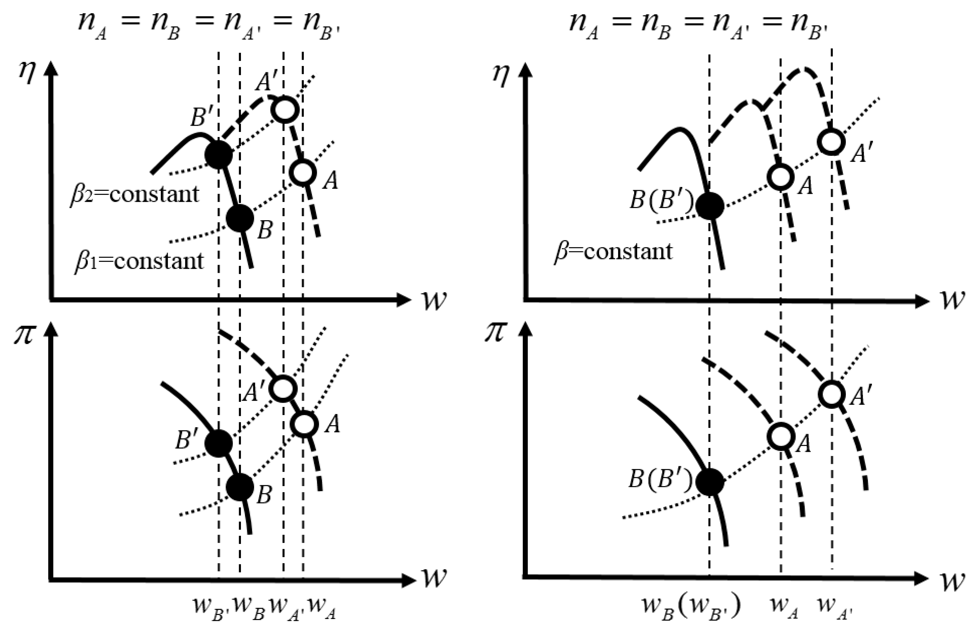
is related to the operating condition and degradation degree of the engine. Figure 4 depicts the variation of the S F caused by the variation of either the operating condition or the degradation degree on a compressor map. The left figure represents an example of the S F changing with the operation condition when the degradation degree remains constant, while the right one is opposite. Therefore, the defined S F represents the characteristic deviations at a certain operating condition and degradation degree.
Usually, engines degrade very slowly during a small temporal scale, such as a day or an hour, in its early life stage. It can be considered that the degradation degree keeps the same attribute. However, the engine’s operating condition varies significantly with the aircraft flight mission. Thus, the influence of the operating condition on the S F exceeds that of the degradation degree and becomes the focus of this paper below.

2.3. Scaling Factor Prediction

By introducing the S F , Equation (1) can be rewritten as Equation (7):
x ˙ = f ( x , u , v , ζ * , S F s ) y = g ( x , u , v , ζ * , S F s )
where vector ζ contains the nominal values of each component’s characteristics, and vector S F s comprises the S F of concerned components.
Undoubtedly, the S F s can be seen as model tuners. When the engine is in deterioration, the actual components’ characteristics can be obtained by using the S F s to modify ζ ; thus, the degraded performance of the real engine can be estimated accurately.
However, the engine inevitably will vary its operating condition. When the operating condition changes, the S F s calculation often corresponds to the operating condition several seconds prior due to the dynamic response of the measurable parameters. Then, employing the S F s directly in Equation (7) would also cause hysteretic estimation results. For performance fast estimation, the S F s at present operating condition should be acquired quickly.
Since the S F s relate to the operating condition, a mapping relationship for each S F with the operating condition is constructed as Equation (8):
{ u , v } S F
With the aid of the mapping relationship established, an algorithm with memory function is designed to predict the S F s at present operating condition. And the prediction problem of each S F can be formulated as:
S F = f S F ( u , v , u , v , S F )
where u , v , and S F mean the operating conditions and their corresponding S F at the past time; u , v , and S F are those at the present time.
The designed algorithm can be divided into two parts: the first is to store the historical data, i.e., u , v , and S F , and the second is to predict the S F at the present time.
During the engine’s operation, measurements are continuously generated. Thus, each S F can be calculated from the measurements continuously. The calculated S F together with its corresponding operating condition forms the mapping relationship as Equation (8) and is regarded as the historical data.
To store the historical data, a grid of N d is generated, where d is the number of parameters in the operating condition, and N is the intervals of each parameter divided in equal proportion. After normalization, the N intervals of each parameter are expressed as [ 0   ,   1 N ) , [ 1 N , 2 N ) , …, [ ( N 1 ) N   ,   1 ] . Then, each section of the grid can be characterized by the interval of d parameters. For each group of u , v , and S F , which section of the grid it belongs to can be judged according to the d parameters in u and v , and the value of the S F can be stored in this section. Each section has a storage space to record M values and adopts a first-in–first-out principle.
To predict the S F at the present time, firstly the corresponding section according to the d parameters in u and v are found, which is the operating condition at the present time. Then, the values in the section are read and the average as the S F at the present time is taken. When the section has no value, the value of the S F at the previous time is maintained. Then, the initial value of S F is set to 1. The prediction result will be transmitted to Equation (7).
By applying the algorithm in parallel multiple times, all the S F s at present operating condition can be acquired. Thus, the ζ in Equation (7) can be modified to the actual characteristics, and the engine performance can be estimated rapidly.
In terms of memory consumption, a double type number takes up 8 bytes. So, the max memory consumption of the algorithm is about 8 M · N d / 1024 kB. It is not difficult to find that the number of parameters has the greatest impact on the memory consumption.
Eliminating irrelevant variables can help to save memory and curtail the computational complexity [
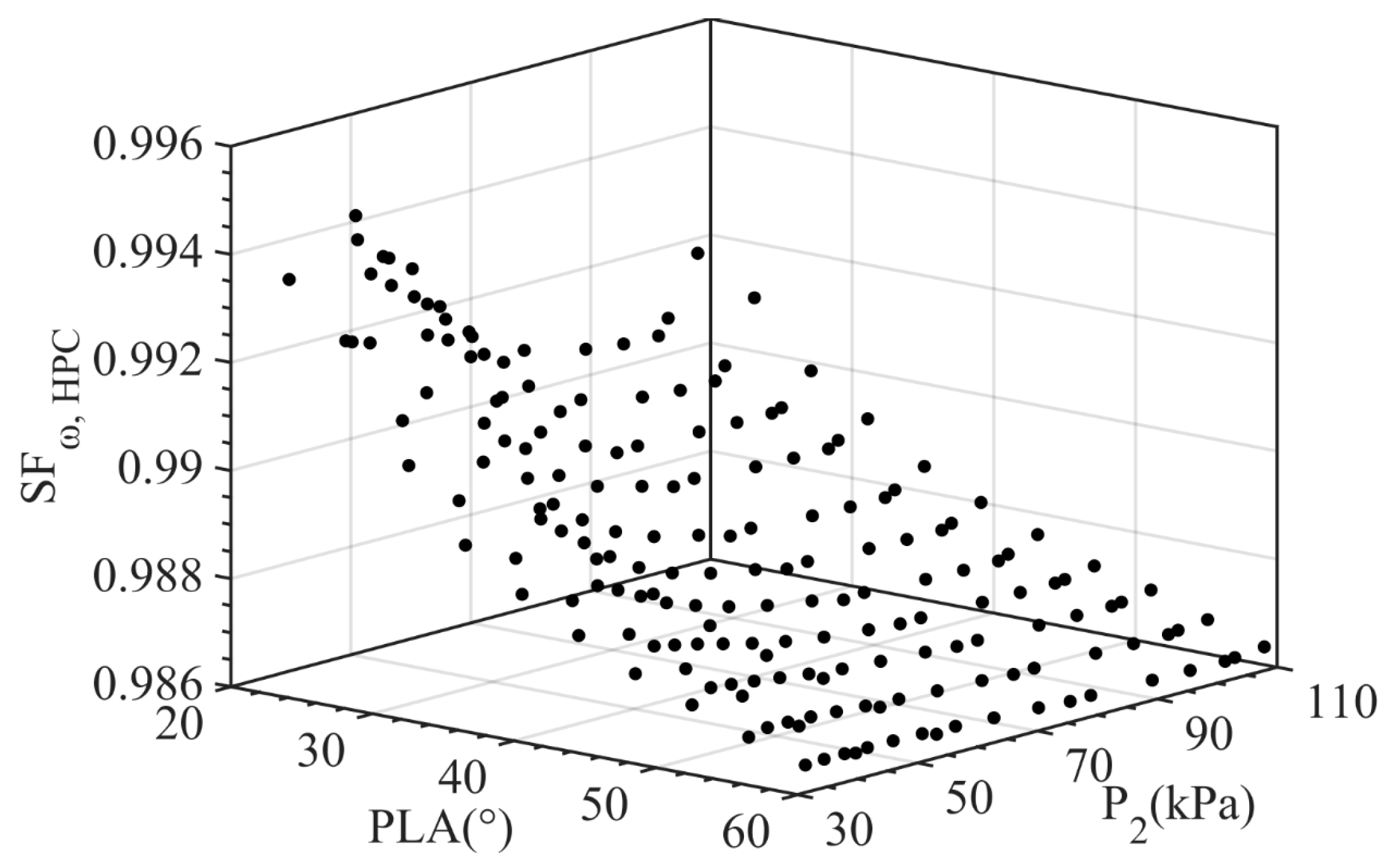
41]. To reveal a concise relationship between the S F and the operating condition, four cases are considered and summarized in Table 1.
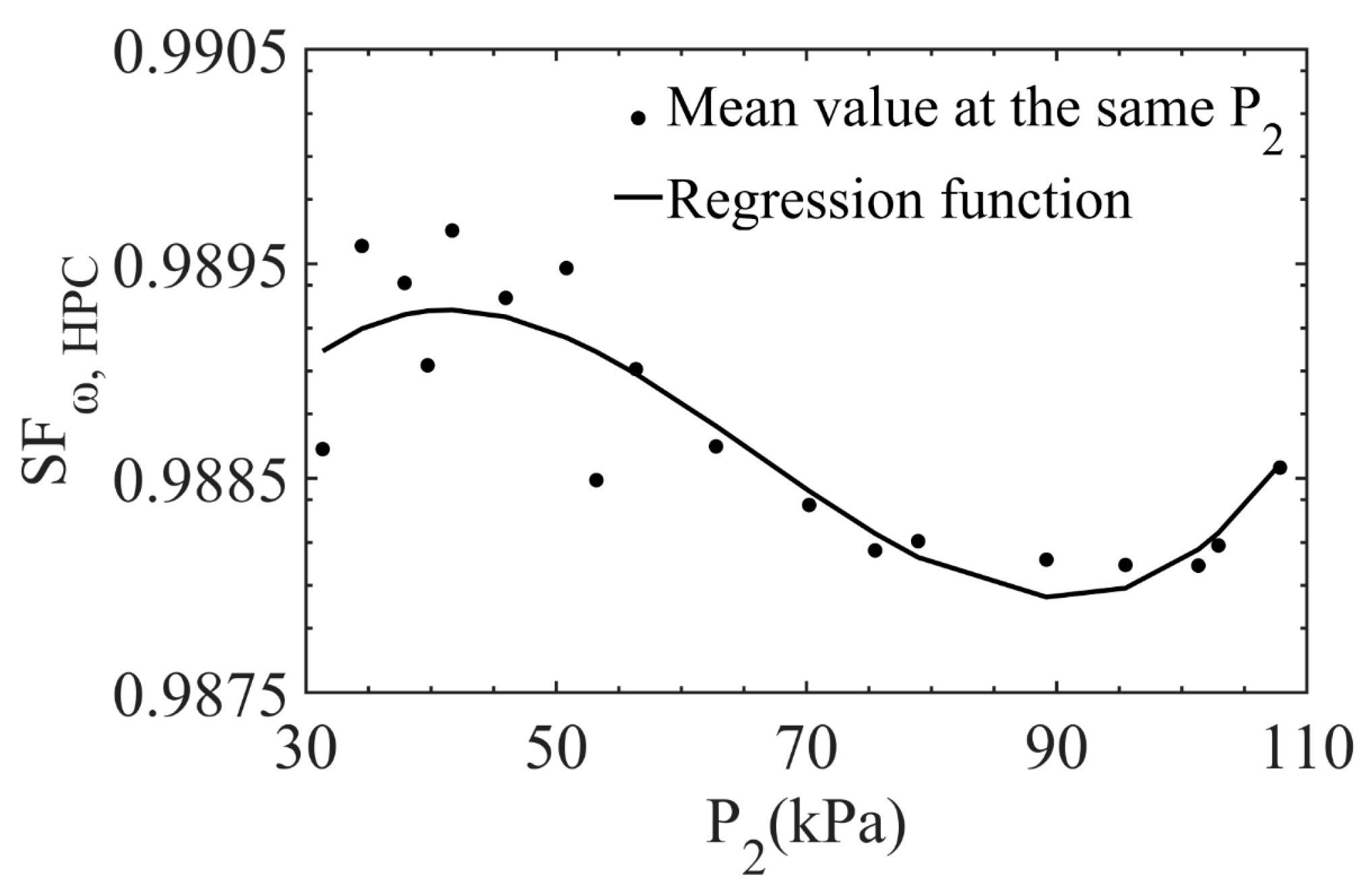
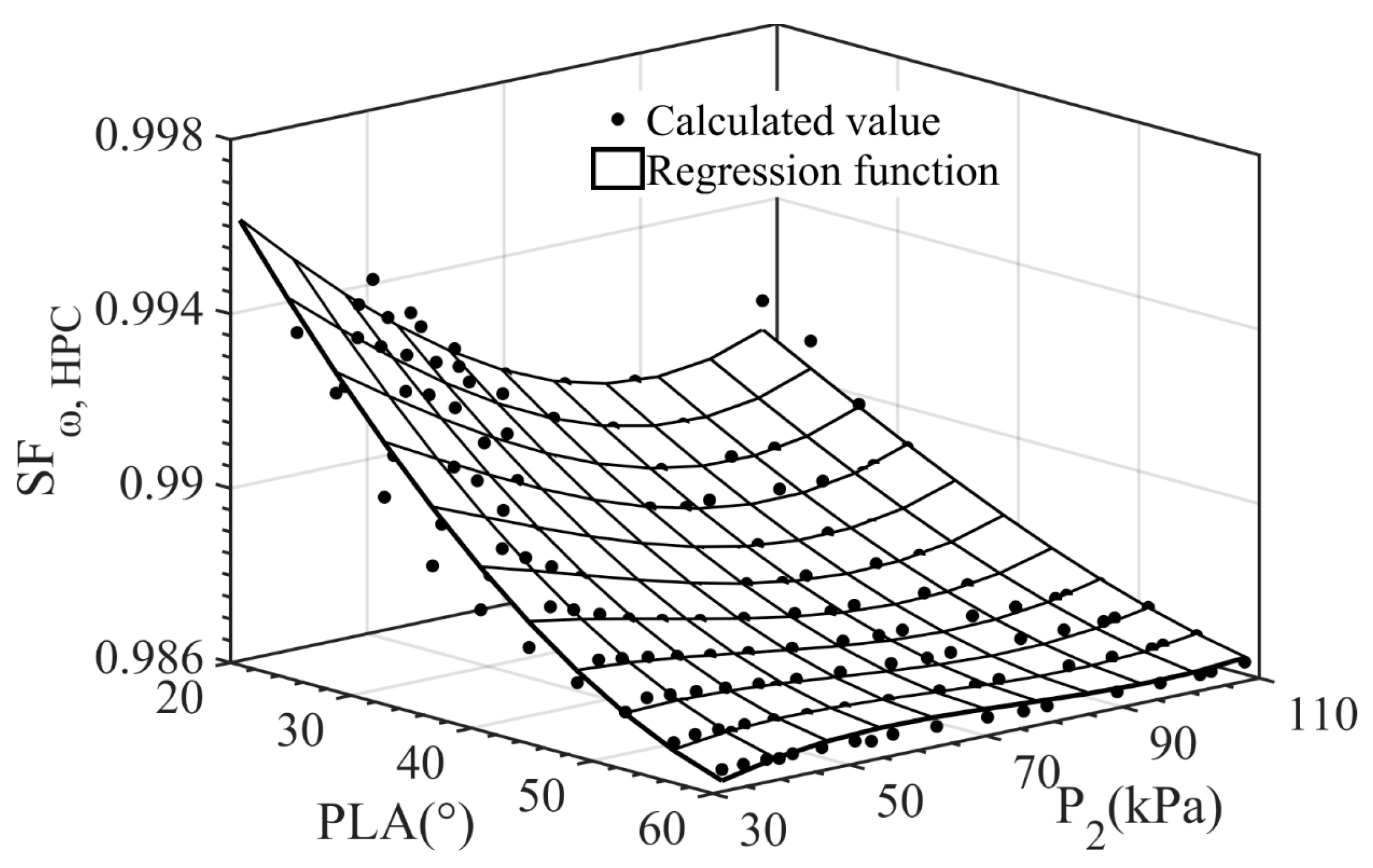
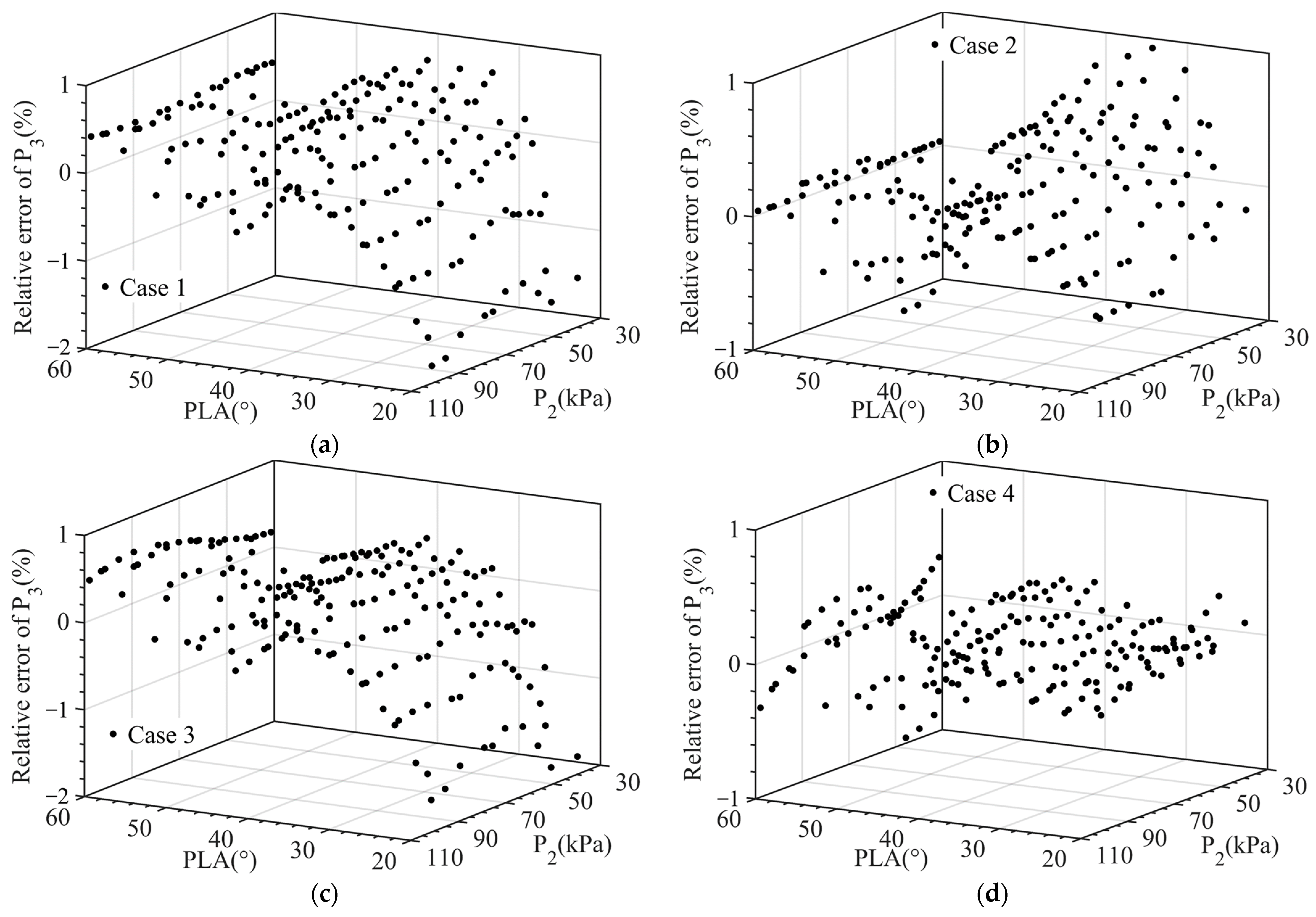
From Case 1 to Case 4, the operating condition in the mapping relationship is considered gradually comprehensive. In Case 1, neither u nor v is included, and the S F is regarded as a constant. Case 2 and Case 3, separately, select u and v of the operating condition to form the mapping relationship. With no simplification, both u and v are involved in the last case.
The case can be determined by comparing the estimation accuracy of multiple operating conditions. Specifically, each operating condition and corresponding calculated S F are reckoned as one sample, and these samples can form a dataset. In the dataset, revealing the mapping relationship of each case is a regression problem. Multivariate polynomial is adopted to solve it. The coefficient and order of the polynomial can be determined based on the least squares principle. All the polynomials will be used to calculate the S F again at these operating conditions, and, thus, the estimation results will be obtained for comparison.

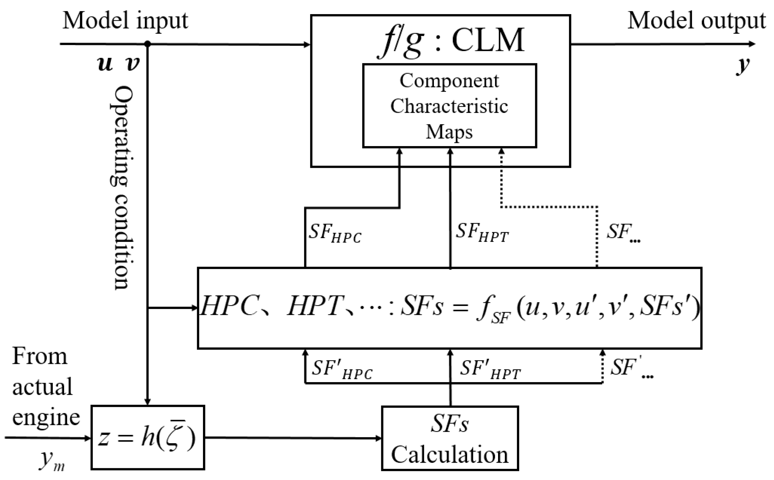
2.4. Onboard Adaptive Model Framework

In combination with the contents of the above subsection, an aeroengine onboard adaptive model for performance fast estimation is established, the framework of which is shown in Figure 5.

3. Simulation and Discussion

For the proposed onboard adaptive model, the self-tuning and fast estimation capability are the main problems that need careful consideration. In this section, simulations in four aspects are implemented to illustrate the self-tuning and fast estimation capability of the model when the engine is in deterioration. Since the target is to demonstrate the effectiveness of the proposed method, it is reasonable to apply the synthetic data in the simulation processes. The engine performance deterioration is imitated by changing the flow capacity and efficiency of different components together. Five major components highlighted in Figure 1 are considered to have degraded flow capacity and efficiency at a certain period, as summarized in Table 2.

3.1. Single Point Accuracy Analysis

In this subsection, the accuracy of the onboard adaptive model at single operating conditions is analyzed. The simulation is firstly implemented at the operating condition (H = 0, Ma = 0, PLA = 60°). Based on the proposed method described in Section 2.1 and Section 2.2, the S F s corresponding to this operating condition are calculated and shown in Table 3. The calculation is under the case of m = n in Section 2.1, and the value of unlisted S F in Table 3 is 1. Then, the outputs of the onboard adaptive model are obtained according to Equation (7). Measurable parameters n l and n h , and unmeasurable parameters inlet temperature of HPC T 4 and net thrust F N , are chosen to compare with those of the actual engine. Another operating condition (H = 11,000 m, Ma = 0.8, PLA = 60°) duplicates the above process. The simulation and comparison results of these two points is described in Table 4.
The results show that the accuracy of the adaptive model is extremely high at these two operating conditions. Obviously, applying the S F s calculated at the operating condition can guarantee the self-tuning capability of the proposed model at single points.

3.2. Multiple Points Accuracy Analysis

A large operating condition range is covered in this subsection to analyze the accuracy of the onboard adaptive model at multiple operating conditions. The setting of the PLA is listed in Table 5. The flight conditions are selected as the red points in Figure 6.
The S F s are calculated at each operating condition. Taking S F ω ,   HPC as an example, its scatter at different operating conditions is displayed in Figure 7. It should be noted that the fan inlet pressure P 2 is used to indicate the flight condition for the convenience of plotting, since the P 2 is a function of the flight condition and uniformly distributed in its range. Other parameters, such as the fan inlet temperature T 2 , can also be adopted.
A tendency that the S F ω ,   HPC varies with the PLA and the P 2 can be obviously seen from Figure 7. But the numerical interval [0.986, 0.995] is quite small. Thus, the classification in Table 1 is reasonable. According to the method described in the last paragraph of Section 2.3, mapping relationships between the S F s and the operating condition are established. Citing the same S F ω , for example, the results of regression analysis are as follows: For Case 1, the S F ω ,   HPC is a constant 0.9887. From Case 2 to Case 4, the functions between the S F ω ,   HPC and the operating condition are displayed in Figure 8, Figure 9, and Figure 10, respectively.
The regression results are fed to the benchmark model. Then, the model is simulated at the above operating conditions. An unmeasurable parameter F N and a measurable parameter P 3 are chosen for comparison with the actual engine. The comparison results of the four cases are shown in Figure 11 and Figure 12.
For the parameter F N , the maximum relative errors of these four cases are 3.85%, 1.04%, 3.46%, and 0.66%, respectively, and the mean relative errors are 0.69%, 0.38%, 0.6%, and 0.21%. These two relative errors are both the largest in Case 1, followed by Case 3 and Case 2, and the smallest in Case 4. In Case 1, the S F s are constant sets. Since the influence of the operating condition on the S F s is not considered, the relative errors change with the PLA and the P 2 , as illustrated in Figure 11a. The maximum relative error appears in the region of small PLA, H, and Ma. In Case 2, the mapping relationships between the S F s and the PLA are established. Since there is a strong linear correlation between the S F and the PLA, as indicated in Figure 8, the accuracy of the adaptive model is improved significantly, compared with Case 1. However, the influence of the flight condition is not considered, so the relative errors fluctuate with the P 2 at the same PLA, as shown in Figure 11b. Compared with Case 2, Case 3 replaces the PLA with the P 2 correspondingly. So, the results of Case 3 are similar to those of Case 2. However, the correlation between the S F and the flight condition is weaker than the PLA, as revealed in Figure 9. The accuracy is, thus, not obviously improved, compared with Case 2. In Case 4, the S F s are functions of the PLA and the P 2 , as shown in Figure 10. Since the influence of the operating condition on the S F s is taken into account thoroughly, small relative errors are obtained in the whole range, as demonstrated in Figure 11d. Similar results of the parameter P 3 can be seen in Table 6.
The above results reveal that Case 4 can achieve better estimation accuracy compared with other cases. In addition, the onboard adaptive model using the mapping relationship of Case 4 is verified to have the self-tuning capability at multiple points. For further verification, an operating condition (H = 1000 m, Ma = 0.05, PLA = 22°), which is not in the aforementioned range, is selected as the test point. In this operating condition, the S F s are calculated based on the four regression functions separately. The simulation and comparison results are shown in Table 7. And the relative errors of this point support the above discussion results.

3.3. Fast Estimation Capability: Response Time Analysis

A scenario including transition is simulated to evaluate the fast estimation capability of the onboard adaptive model. In the scenario, the operating condition is implemented as follows: The flight condition is H = 0 and Ma = 0, and the PLA is given in Figure 13.
Based on the mapping relationships of Case 4, the S F s are predicted by the algorithm with memory function and then applied to the onboard adaptive model. For comparison, an adaptive model using the Kalman filter is established by referring to [15] and a data-driven adaptive model by referring to [28]. The simulation results are shown in Figure 14, taking the unmeasurable parameter F N , for example.
The simulation process contains several transitions. When the engine operating state changes after a transition, the adaptive models need to be updated so that they can estimate the changed parameters. For example, a transition locates at 20–22 s. When the engine enters a new steady state at 22 s, the relative errors of the proposed model, the Kalman filter-based model and the data-driven model, are −0.28%, −1.93%, and −1.6%, respectively, comparing the estimated results with the actual engine. The proposed model has higher accuracy at the initial stage of estimation. From the first two panels in the figure, it can be seen that the dynamic response time of these three models is 0.3 s, 6.5 s, and 9 s, separately. The proposed model has a much shorter estimation time. When the adaptive models enter the steady state, the relative errors of the proposed model and the Kalman filter-based model are almost 0, while the relative error of the data-driven model is 0.05%, as the third panel shows. This may be caused by the lack of training data, which is exactly a disadvantage of the data-driven methods. Compared with the other two methods, the proposed method has a much shorter dynamic response time and, thus, a shorter period of model mismatch. Besides that, the proposed method also has a higher estimation accuracy in the self-tuning process. The above results show that the proposed method has the capability of fast estimation.

3.4. Fast Estimation Capability: Memory Ability Analysis

For the proposed method, the change of each S F in the simulation process of Section 3.3 is shown in Figure 15, taking the S F ω ,   HPC , for example.
Based on the S F calculated by the method described in Section 2.1 and 2.2 (the black line), the S F at present operating condition can be predicted as the red line in Figure 15. The employed algorithm has the memory ability to deal with historical data. At 22 s, since there is no historical data of this state, the predicted S F takes the value of the previous time and causes a slight deviation from the actual value. While at 62 s, there is a great quantity of historical data at 22–40 s, so the predicted S F directly derives the actual value. Correspondingly, the estimation result has a small relative error at 22 s, whereas the actual thrust is almost immediately estimated at 62 s, as shown in the first and fourth panels of Figure 14. In addition, it is obvious to find from these panels that the Kalman filter-based model and the data-driven model repeat their previous self-tuning process. Compared with the other two methods, the proposed method has the memory function to avoid a repeated estimation process, and the fast estimation capability of the proposed model is thus enhanced.

4. Conclusions

In this paper, an onboard adaptive model with fast estimation capability is proposed. Considering that a benchmark model can be adapted to the actual engine by employing some tuners, a component level model is constructed, and some scaling factors are introduced. The scaling factors can be derived from the measurements and are represented as mapping relationships with the operating condition. An algorithm with memory function is designed to rapidly obtain the scaling factors at the present operating condition. Finally, feeding the scaling factors to the benchmark model, the engine performance can be estimated accurately and quickly. Simulation scenarios are implemented to illustrate the effectiveness of the proposed model. The results are as follows:
(1) By employing the S F s as the model tuners, the proposed model has high estimation accuracy at both single points and multiple points when the engine is in deterioration. The relative errors of the model are almost 0 at single points and no more than 0.66% at multiple points.
(2) The correlation between the S F and the operating condition is thoroughly considered. Representing the S F as a function of u and v can achieve a better estimation accuracy compared with other cases.
(3) Compared with the Kalman-based and the data-driven methods, the proposed model has smaller relative errors and shorter dynamic response time when the engine varies the operating state. With the aid of an algorithm with memory function, the proposed model can avoid repeated self-tuning processes.
Overall, all the results demonstrate that the proposed model has self-tuning and fast estimation capability and is a potential for application in engine control, monitoring, and diagnostics.

Author Contributions

Conceptualization, Z.J. and S.Y.; methodology, Z.J. and X.W.; software, Z.J. and S.Y.; validation, X.W. and Y.L.; formal analysis, Z.J.; investigation, S.Y.; resources, X.W.; data curation, Z.J.; writing—original draft preparation, Z.J.; writing—review and editing, S.Y. and Y.L.; visualization, Z.J.; supervision, S.Y.; project administration, X.W.; funding acquisition, X.W. All authors have read and agreed to the published version of the manuscript.

Funding

This research was funded by National Science and Technology Major Project (J2019-V-0010-0104).

Data Availability Statement

Data are contained within the article.

Conflicts of Interest

The authors declare no conflict of interest.

References

  1. Ru, P.; Subbarao, K. Nonlinear model predictive control for unmanned aerial vehicles. Aerospace 2017, 4, 31. [Google Scholar] [CrossRef]
  2. Chen, H.; Zheng, Q.; Gao, Y.; Zhang, H. Performance seeking control of minimum infrared characteristic on double bypass variable cycle engine. Aerosp. Sci. Technol. 2021, 108, 106359. [Google Scholar] [CrossRef]
  3. Zhu, Y.Y.; Huang, J.Q.; Pan, M.X.; Zhou, W. Direct thrust control for multivariable turbofan engine based on affine linear parameter-varying approach. Chin. J. Aeronaut. 2022, 35, 125–136. [Google Scholar] [CrossRef]
  4. Fentaye, A.D.; Baheta, A.T.; Gilani, S.I.; Kyprianidis, K.G. A review on gas turbine gas-path diagnostics: State-of-the-art methods, challenges and opportunities. Aerospace 2019, 6, 83. [Google Scholar] [CrossRef] [Green Version]
  5. Wang, Y.; Zheng, Q.G.; Du, Z.Y.; Zhang, H.B. Research on nonlinear model predictive control for turboshaft engines based on double engines torques matching. Chin. J. Aeronaut. 2020, 33, 561–571. [Google Scholar] [CrossRef]
  6. Zhou, X.; Lu, F.; Huang, J.Q. Fault diagnosis based on measurement reconstruction of HPT exit pressure for turbofan engine. Chin. J. Aeronaut. 2019, 32, 1156–1170. [Google Scholar] [CrossRef]
  7. Cruz-Manzo, S.; Panov, V.; Zhang, Y. Gas path fault and degradation modelling in twin-shaft gas turbines. Machines 2018, 6, 43. [Google Scholar] [CrossRef] [Green Version]
  8. Yang, S.B.; Alafate, J.; Wang, X.; Tian, Z. A Self-Tuning Model Framework Using K-Nearest Neighbors Algorithm. In Turbo Expo: Power for Land, Sea, and Air; American Society of Mechanical Engineers: New York, NY, USA, 2020; Volume 84140, p. V005T05A019. [Google Scholar]
  9. Yang, X.; Guo, X.; Dong, W. On-Line Component Map Adaptive Procedure Based on Sensor Data. In Turbo Expo: Power for Land, Sea, and Air; American Society of Mechanical Engineers: New York, NY, USA, 2020; Volume 84058, p. V001T01A041. [Google Scholar]
  10. Ma, Y.H.; Du, X.; Sun, X.M. Adaptive modification of turbofan engine nonlinear model based on LSTM neural networks and hybrid optimization method. Chin. J. Aeronaut. 2022, 35, 314–332. [Google Scholar] [CrossRef]
  11. Zhou, G.T.; Su, S.M. Application of Improved Extended Kalman Filter for Adaptive Model of Aircraft Engine. Appl. Mech. Mater. 2015, 709, 180–185. [Google Scholar] [CrossRef]
  12. Luppold, R.; Roman, J.; Gallops, G.; Kerr, L. Estimating in-flight engine performance variations using Kalman filter concepts. In Proceedings of the 25th Joint Propulsion Conference, Monterey, CA, USA, 12–16 July 1989; p. 2584. [Google Scholar]
  13. Brotherton, T.; Volponi, A.; Luppold, R.; Simon, D.L. eSTORM: Enhanced Self Tuning On-Board Real-Time Engine Model; Intelligent Automation Corp.: Poway, CA, USA, 2003. [Google Scholar]
  14. Panov, V. Model-based control and diagnostic techniques for operational improvements of gas turbine engines. In Proceedings of the 10th European Turbomachinery Conference, Lappeenranta, Finland, 15–19 April 2013; pp. 15–19. [Google Scholar]
  15. Panov, V. Auto-tuning of real-time dynamic gas turbine models. In Turbo Expo: Power for Land, Sea, and Air; American Society of Mechanical Engineers: Düsseldorf, Germany, 2014; Volume 45752, p. V006T06A004. [Google Scholar]
  16. Simon, D. A comparison of filtering approaches for aircraft engine health estimation. Aerosp. Sci. Technol. 2008, 12, 276–284. [Google Scholar] [CrossRef]
  17. Volponi A, J. Use of hybrid engine modeling for on-board module performance tracking. In Turbo Expo: Power for Land, Sea, and Air; American Society of Mechanical Engineers: Reno, NV, USA, 2005; Volume 46997, pp. 525–533. [Google Scholar]
  18. Pang, S.; Li, Q.; Feng, H. A hybrid onboard adaptive model for aero-engine parameter prediction. Aerosp. Sci. Technol. 2020, 105, 105951. [Google Scholar] [CrossRef]
  19. Daum, F. Nonlinear filters: Beyond the Kalman filter. IEEE Aerosp. Electron. Syst. Mag. 2005, 20, 57–69. [Google Scholar] [CrossRef]
  20. Ribeiro, M.I. Kalman and extended kalman filters: Concept, derivation and properties. Inst. Syst. Robot. 2004, 43, 46. [Google Scholar]
  21. Gośliński, J.; Giernacki, W.; Królikowski, A. A nonlinear filter for efficient attitude estimation of unmanned aerial vehicle (UAV). J. Intell. Robot. Syst. 2019, 95, 1079–1095. [Google Scholar] [CrossRef] [Green Version]
  22. Gośliński, J.; Kasiński, A.; Giernacki, W.; Owczarek, P.; Gardecki, S. A study on coaxial quadrotor model parameter estimation: An application of the improved square root unscented Kalman filter. J. Intell. Robot. Syst. 2019, 95, 491–510. [Google Scholar] [CrossRef] [Green Version]
  23. Brunell, B.J.; Viassolo, D.E.; Prasanth, R. Model adaptation and nonlinear model predictive control of an aircraft engine. In Turbo Expo: Power for Land, Sea, and Air; American Society of Mechanical Engineers: Vienna, Austria, 2004; Volume 41677, pp. 673–682. [Google Scholar]
  24. Dewallef, P.; Léonard, O. On-line performance monitoring and engine diagnostic using robust Kalman filtering techniques. In Turbo Expo: Power for Land, Sea, and Air; American Society of Mechanical Engineers: Atlanta, GA, USA, 2003; Volume 36843, pp. 395–403. [Google Scholar]
  25. Yang, Z.X.; Huang, J.Q.; Feng, L.U. Kalman Filter for Aero-Engine Health Parameter Estimation Analysis. Gas Turbine Exp. Res. 2012, 25, 41–43. [Google Scholar]
  26. Kobayashi, T.; Simon, D.L. Hybrid neural-network genetic-algorithm technique for aircraft engine performance diagnostics. J. Propuls. Power 2005, 21, 751–758. [Google Scholar] [CrossRef]
  27. Wang, X.D.; Sun, J.G.; Li, S.L. Application of neural networks to areoengine adaptive modeling. J. Aerosp. Power 2003, 18, 845–849. [Google Scholar]
  28. Wang, J.; Zhang, H.; Yan, C.; Duan, S.; Huang, X. An adaptive turbo-shaft engine modeling method based on PS and MRR-LSSVR algorithms. Chin. J. Aeronaut. 2013, 26, 94–103. [Google Scholar] [CrossRef] [Green Version]
  29. Kim, S.; Kim, K.; Son, C. Transient system simulation for an aircraft engine using a data-driven model. Energy 2020, 196, 117046. [Google Scholar] [CrossRef]
  30. Cesa-Bianchi, N.; Conconi, A.; Gentile, C. On the generalization ability of on-line learning algorithms. IEEE Trans. Inf. Theory 2004, 50, 2050–2057. [Google Scholar] [CrossRef]
  31. Chapman, J.W.; Lavelle, T.M.; May, R.D.; Litt, J.S.; Guo, T.H. Toolbox for the Modeling and Analysis of Thermodynamic Systems (T-MATS) User’s Guide; Vantage Partners, LLC: Cleveland, OH, USA.
  32. Visser, W.P.; Broomhead, M.J. GSP, a generic object-oriented gas turbine simulation environment. In ASME Turbo Expo 2000: Power for Land, Sea, and Air; American Society of Mechanical Engineers: Munich, Germany, 2000. [Google Scholar]
  33. Urban, L.A. Parameter selection for multiple fault diagnostics of gas turbine engines. J. Eng. Power 1975, 97, 225–230. [Google Scholar] [CrossRef]
  34. Blinstrub, J.; Li, Y.G.; Newby, M.; Zhou, Q.; Stigant, G.; Pilidis, P.; Hönen, H. Application of gas path analysis to compressor diagnosis of an industrial gas turbine using field data. In Turbo Expo: Power for Land, Sea, and Air; American Society of Mechanical Engineers: Düsseldorf, Germany, 2014; Volume 45653, p. V03AT07A008. [Google Scholar]
  35. Li, Y.G.; Pilidis, P.; Newby, M.A. An Adaptation Approach for Gas Turbine Design-Point Performance Simulation. J. Eng. Gas Turbines Power 2006, 128, 789–795. [Google Scholar] [CrossRef]
  36. Verbist, M.L.; Visser, W.P.J.; van Buijtenen, J.P. Experience with gas path analysis for on-wing turbofan condition monitoring. J. Eng. Gas Turbines Power 2014, 136, 011204. [Google Scholar] [CrossRef]
  37. Kurzke, J.; Halliwell, I. Propulsion and Power: An Exploration of Gas Turbine Performance Modeling; Springer International Publishing: Cham, Switzerland, 2018. [Google Scholar]
  38. Stamatis, A.; Mathioudakis, K.; Papailiou, K.D. Adaptive simulation of gas turbine performance. J. Eng. Gas Turbines Power 1990, 112, 168–175. [Google Scholar] [CrossRef]
  39. Borguet, S.; Léonard, O. Comparison of adaptive filters for gas turbine performance monitoring. J. Comput. Appl. Math. 2010, 234, 2202–2212. [Google Scholar] [CrossRef] [Green Version]
  40. Lu, S.; Zhou, W.; Huang, J.; Lu, F.; Chen, Z. A Novel Performance Adaptation and Diagnostic Method for Aero-Engines Based on the Aerothermodynamic Inverse Model. Aerospace 2021, 9, 16. [Google Scholar] [CrossRef]
  41. Zhao, Y.P.; Sun, J.G. Thrust estimator design based on least squares support vector regression machine. J. Harbin Inst. Technol. 2010, 17, 578–583. [Google Scholar]
Figure 1. Schematic of typical civil high-bypass twin-shaft turbofan engine8.
Aerospace 09 00845 g001
Figure 2. Iteration process of actual characteristics calculation.
Aerospace 09 00845 g002
Figure 3. Definition of scaling factor on a compressor map.
Aerospace 09 00845 g003
Figure 4. The change of the S F with the operating condition or the degradation degree on a compressor map.
Aerospace 09 00845 g004
Figure 5. The framework of proposed onboard adaptive model.
Aerospace 09 00845 g005
Figure 6. Model input v : Selection of the flight condition.
Aerospace 09 00845 g006
Figure 7. The scatter of the S F ω ,   HPC .
Aerospace 09 00845 g007
Figure 8. Regression analysis result of the mapping relationship: Case 2.
Aerospace 09 00845 g008
Figure 9. Regression analysis result of the mapping relationship: Case 3.
Aerospace 09 00845 g009
Figure 10. Regression analysis result of the mapping relationship: Case 4.
Aerospace 09 00845 g010
Figure 11. Relative errors of the parameter F N .
Aerospace 09 00845 g011aAerospace 09 00845 g011b
Figure 12. Relative errors of the parameter P 3 .
Aerospace 09 00845 g012
Figure 13. The variation of PLA in the simulation.
Aerospace 09 00845 g013
Figure 14. Simulation results of the parameter F N .
Aerospace 09 00845 g014
Figure 15. Prediction results of the S F ω ,   HPC .
Aerospace 09 00845 g015
Table 1. Summary of the mapping relationship cases between the S F and the operating condition.
CaseMapping Relationship
1 SF = constant
2 SF = f S F ( u )
3 SF = f S F ( v )
4 SF = f S F ( u , v )
Table 2. Assumed degradation of the concerned component.
Flow CapacityEfficiency
Fan95%95%
BST97%95%
HPC98%95%
HPT96%95%
LPT97%95%
Table 3. The S F s of operating condition (H = 0, Ma = 0, PLA = 60°).
SFFanSFBSTSFHPCSFHPTSFLPT
S F ω
S F π
S F η
S F ω
S F π
S F η
S F ω
S F π
S F η
S F ω
S F η
S F ω
S F η
0.960.9790.9370.9860.9940.9520.9860.9850.9490.960.950.970.95
Table 4. Simulation and comparison results at single points.
Operating ConditionParametersValue
Adaptive ModelActual EngineRelative Error (%)
H = 0, Ma = 0, PLA = 60° n l (%)1001000
n h (%)99.5199.510
T 4 (K)1672.4281672.4278.9 × 10−5
F N (N)245,004.86245,004.821.95 × 10−5
H = 11,000 m, Ma = 0.8, PLA = 60° n l (%)92.1292.120
n h (%)91.0591.050
T 4 (K)1429.6771429.6779.15 × 10−6
F N (N)111,016.22111,016.224.54 × 10−7
Table 5. Model input u : Command of the PLA.
No.PLA (°)No.PLA (°)
120744
224848
328952
4321056
5361160
640
Table 6. Relative errors (absolute value) of parameters F N and P 3 .
ParameterRelative ErrorCase
1234
F N max (%)3.851.043.460.66
mean (%)0.690.380.60.21
P 3 max (%)1.81.151.80.48
mean (%)0.390.260.370.15
Table 7. Simulation and comparison results of operating condition (H = 1000 m, Ma = 0.05, PLA = 22°).
FN (N)Relative Error (%)P3 (kPa)Relative Error (%)
Actual engine49,541.24 845.958
Adaptive model: Case 147,064.88−5823.594−2.64
Adaptive model: Case 249,145.35−0.8842.878−0.36
Adaptive model: Case 347,302.22−4.52825.142−2.46
Adaptive model: Case 449,511.37−0.06845.616−0.04
Publisher’s Note: MDPI stays neutral with regard to jurisdictional claims in published maps and institutional affiliations.

