Article

Image Quality Enhancement with Applications to Unmanned Aerial Vehicle Obstacle Detection

1
College of Astronautics, Nanjing University of Aeronautics and Astronautics, 29 Jiangjun Street, Nanjing 211106, China
2
Department of Mechanical Engineering, University of Canterbury, 4800 Private Bag, Christchurch 8140, New Zealand
*
Author to whom correspondence should be addressed.
Aerospace 2022, 9(12), 829; https://doi.org/10.3390/aerospace9120829
Submission received: 10 November 2022 / Revised: 8 December 2022 / Accepted: 11 December 2022 / Published: 15 December 2022

Abstract

:
Aiming at the problem that obstacle avoidance of unmanned aerial vehicles (UAVs) cannot effectively detect obstacles under low illumination, this research proposes an enhancement algorithm for low-light airborne images, which is based on the camera response model and Retinex theory. Firstly, the mathematical model of low-illumination image enhancement is established, and the relationship between the camera response function (CRF) and brightness transfer function (BTF) is constructed by a common parameter equation. Secondly, to solve the problem that the enhancement algorithm using the camera response model will lead to blurred image details, Retinex theory is introduced into the camera response model to design an enhancement algorithm framework suitable for UAV obstacle avoidance. Thirdly, to shorten the time consumption of the algorithm, an acceleration solver is adopted to calculate the illumination map, and the exposure matrix is further calculated via the illumination map. Additionally, the maximum exposure value is set for low signal-to-noise ratio (SNR) pixels to suppress noise. Finally, a camera response model and exposure matrix are used to adjust the low-light image to obtain an enhanced image. The enhancement experiment for the constructed dataset shows that the proposed algorithm can significantly enhance the brightness of low-illumination images, and is superior to other similar available algorithms in quantitative evaluation metrics. Compared with the illumination enhancement algorithm based on infrared and visible image fusion, the proposed algorithm can achieve illumination enhancement without introducing additional airborne sensors. The obstacle object detection experiment shows that the proposed algorithm can increase the AP (average precision) value by 0.556.

1. Introduction

With the development of unmanned aerial vehicle (UAV) technology, UAVs are widely used in aerial photography, smart agriculture, package delivery, remote sensing, and power line inspection. These widespread applications have led to an increasing number of UAVs in low-altitude airspace, increasing the risk of collisions between UAVs. Therefore, it is vital to ensure the safety of UAVs during their missions, i.e., avoid collisions between different UAVs.
Machine vision, as an intelligent technology, has been widely researched and succeeded in the fields of space robots [1], unmanned vehicles [2], micro air vehicles [3], and fixed-wing aircraft automatic landing [4].
Research on machine vision in unmanned aerial vehicles (UAVs) focuses on the following aspects
(1)
Vision-based positioning method [5];
(2)
Vision-based autonomous UAV landing [6];
(3)
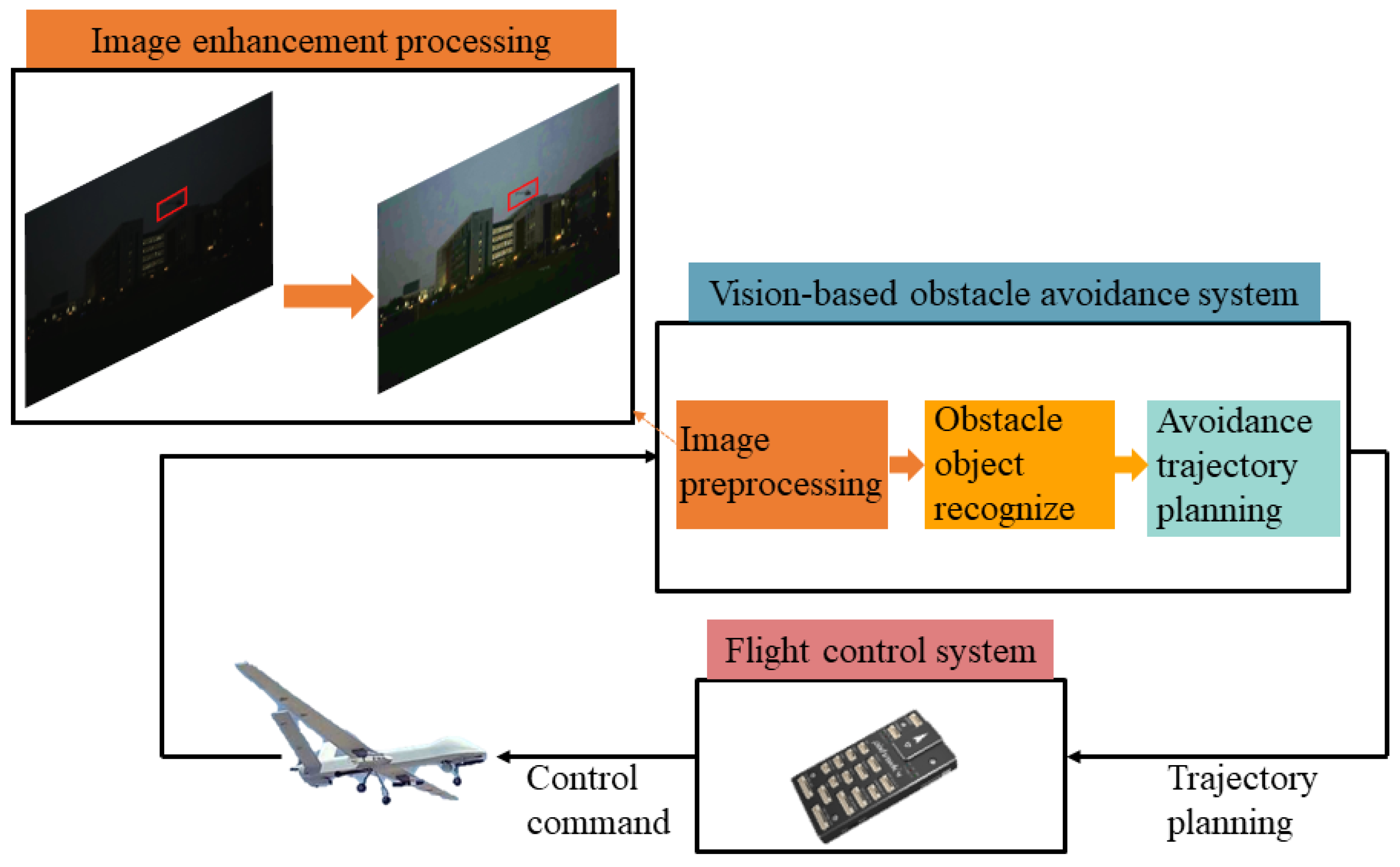
Vision-based obstacle avoidance [7].
Vision-based obstacle avoidance is considered a viable technique for avoiding low-altitude collisions between UAVs. Generally, vision-based obstacle avoidance contains two parts: (1) obstacle perception, which aims to detect obstacles (other UAV) that may threaten the safety of UAV flight; (2) avoidance trajectory planning, which aims to replan a safety trajectory that can avoid obstacles.
Figure 1 presents a typical configuration of a common vision-based obstacle perception and avoidance system.
As shown in Figure 1, high-quality images are the prerequisite to ensure the effectiveness of obstacle avoidance. However, many missions require UAVs to perform at night, and poor lighting in night-time environments can severely affect their ability to sense obstacles and increase the risk of flight. Therefore, it is usually necessary to preprocess the image to enhance image brightness. In present days, image defogging, image dust removal, and brightness enhancement are widely studied algorithms for image preprocessing. Li et al. [8] proposed a method to eliminate the effect of dust on visual navigation during a Mars landing. González et al. [9] processed the low-resolution image acquired by a UAV based on the super-resolution technology of convolutional neural network (CNN) to obtain the high-resolution image. Zhao et al. [10] investigated the application of image-defogging technology in UAV visual navigation. Zhang et al. [11] studied a defogging method based on significance-guided dual-scale transmission correction. Wang et al. [12] utilized the double tangent curve to enhance the brightness of pedestrian photos acquired by UAV in night-time environments. Gao et al. [13] presented a new atmospheric scattering model to defog UAV remote sensing images obtained in hazy weather.
In general, image defogging and image dedusting algorithms, despite some differences in implementation details, can both be grouped into the same class of problems, i.e., eliminating the impact of suspended atmospheric particles (e.g., water droplets, sand, and dust) on image quality. In contrast, the image brightness enhancement algorithm has its own particular goals. Its core purpose is to adjust the exposure of the low-brightness pixel position to achieve image brightness enhancement. Existing low-brightness image enhancement algorithms can be grouped into two categories: brightness enhancement using a single visible image, and brightness enhancement by fusing infrared and visible images.
Brightness enhancement algorithms based on a single visible image contain the following aspects
(1)
Histogram equalization-based algorithms, its core idea is to extend the image dynamic range by adjusting the histogram, so that the darker areas of the image are visible. Its main advantages are simple and high in efficiency, whereas the disadvantage is that this kind of algorithm is not flexible enough for adjusting the local area of the image, which can easily lead to under-exposure/over-exposure and noise amplification in the local area of the image. Representative algorithms include contrast-accumulated histogram equalization (CAHE) [14], brightness-preserving dynamic histogram equalization (BPDHE) [15], etc.
(2)
Defogging-based algorithms, these algorithms first invert the image, then apply the defogging algorithm to the inverted image, and finally invert the defogged image to obtain an enhanced image. The basic model used by this kind of algorithm lacks reasonable physical explanation, and its use of denoising techniques as post-processing will result in the blurring of image details. Representative algorithms include adaptive multiscale retinex (AMSR) [16], ENR [17], etc.
(3)
Statistical model-based algorithms, this kind of algorithm utilizes a statistical model to characterize the ideal attributes of an image. The effectiveness of such algorithms relies on prior knowledge of the statistical model. When the assumptions are exceeded, such as strong noise in the input image, the adaptability of such algorithms is insufficient. Representative algorithms include bio-inspired multi-exposure fusion (BIMEF) [18].
(4)
Retinex-based algorithms, this kind of algorithm breaks down the image into two components, a reflectance map and an illumination map, and further processes these two components to obtain the enhancement image. The main advantage of such algorithms is that they can dynamically process images and achieve adaptive enhancement for various images. However, their disadvantage is that such algorithms remove illumination by default and do not limit the range of reflectance, so they cannot effectively maintain the naturalness of the image. Representative algorithms include joint enhancement and denoising (JED) [19], low-light image enhancement (LIME) [20], multiple image fusion (MF) [21], Robust [22], etc.
(5)
Deep learning-based algorithms, this kind of algorithm enhances an image by the relationship between the poor brightness image and the well-exposed image which is obtained by training a deep neural network. The extraction of powerful prior information from large-scale data gives this algorithm a general performance advantage. However, those algorithms have high computational complexity, are time-consuming, and require large datasets. Representative algorithms include enhancement via edge-enhanced multi-exposure fusion network (EEMEFN) [23], Zero-reference deep curve estimation (Zero DCE) [24], etc.
Although the aforementioned algorithms have achieved varying degrees of success on open datasets such as LIME [20] and ExDark [25], their limitations are as follows. (1) The above algorithms rely on iterative optimization in calculating the illumination map, which is time-consuming and therefore cannot satisfy the requirements of real-time processing for UAV obstacle avoidance. (2) Deep learning-based algorithms need to rely on a high volume of paired low/normal brightness image datasets for network training. For the application scenarios of UAV obstacle avoidance, there is currently a lack of large pairs of low/normal brightness datasets containing UAV obstacle objects, so this kind of algorithm cannot be applied to UAV obstacle avoidance scenarios. (3) The camera model lacks a reasonable physical explanation, which can easily result in blurred image details, and some algorithms are not flexible enough to adjust the low signal-to-noise ratio (SNR) area of the image, which can easily lead to under-exposure/over-exposure and noise expansion. Images with blurred details and noise expansion are not conducive to accurate object recognition in the UAV obstacle avoidance process.
Brightness enhancement algorithms based on infrared and visible image fusion include multi-scale transform-based algorithms [26,27], sparse representation-based algorithms [28,29], deep learning-based algorithms [30,31], and so on. Its core idea is to integrate the superiority of infrared and visible images by complementing each other, to achieve brightness enhancement. The brightness enhancement algorithm via fusing the infrared and visible images needs to introduce additional sensors that cannot meet the load requirements of small UAVs.
To eliminate the limitation of a low-illumination environment on the vision-based obstacle avoidance of unmanned aerial vehicles, this paper proposes a low-brightness airborne image enhancement algorithm utilizing the camera response model and the Retinex theory. While comparing with the existing brightness enhancement algorithms, the proposed algorithm has the following advantages.
(1) Solving the problem of blurred image details caused by existing enhancement algorithms, a low-light image enhancement algorithm framework for UAV obstacle avoidance is designed and combined with Retinex theory.
(2) Solving the problem that the pixel position with a low SNR value is easy to generate noise in the enhancement process of the existing algorithm, the maximum exposure threshold is set for the low SNR pixel position.
(3) Solving the problem that the calculation process of the illumination map depends on iterative optimization and is time-consuming, this study utilizes an accelerated solver to compress the solution space to reduce the time consumption.
The remainder of this article is structured below. The mathematical model of the airborne image enhancement algorithm is presented in Section 2. Section 3 presents the improved image enhancement algorithm designed for UAV obstacle avoidance. In Section 4, simulation results and analysis are presented. Section 5 summarizes the work of this paper.

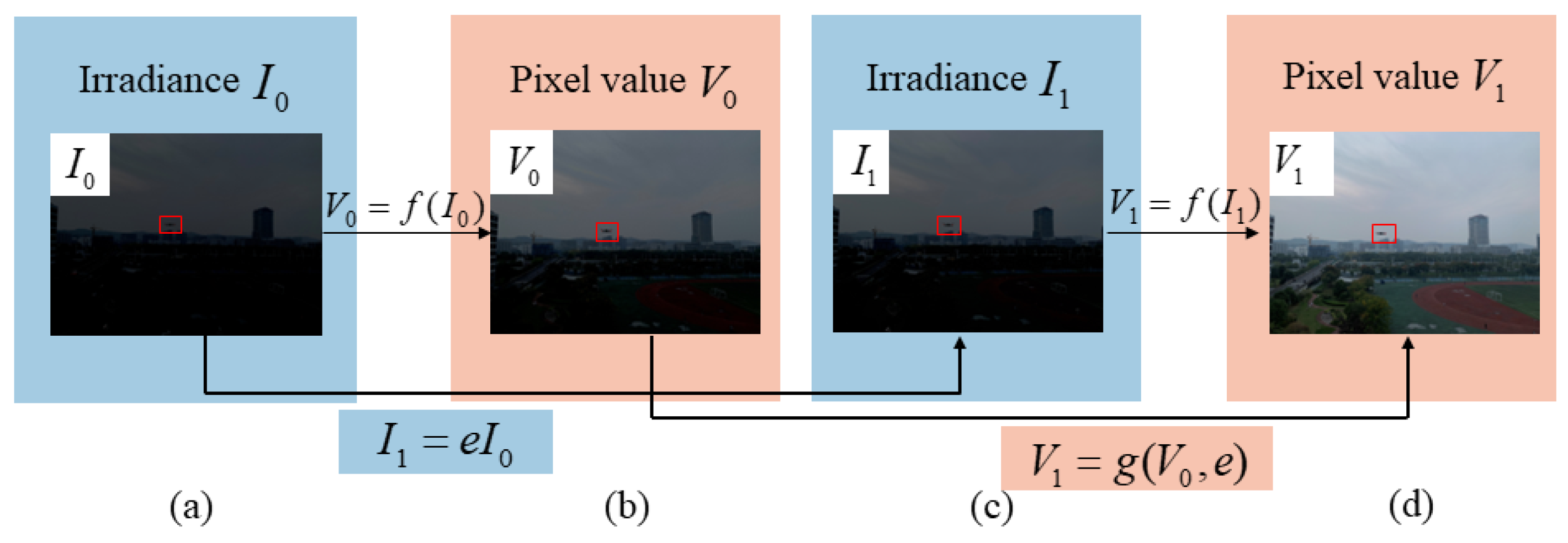
2. Mathematical Model of Scene Brightness Described by Image

The core work of this paper is to improve the brightness of low-light images. Therefore, it is necessary to first establish a mathematical model for describing scene brightness, as shown in Equation (1). For a single image, the relationship between the image irradiance I and the pixel value V of each pixel can be expressed by a nonlinear function f, which is the camera response function (CRF).
V = f ( I )
Generally, the irradiance I reaching the camera sensor changes linearly with the change of the camera exposure parameters. Because the camera performs nonlinear processing on the response of irradiance, the image pixel values V do not change linearly with the irradiance I, so it is needed to use a nonlinear function to characterize the mapping relationship between images with different irradiance. We use the brightness transfer function (BTF), which is represented by g, to define the mapping relationship. As shown in Equation (2), g defines the nonlinear relationship between the image V 0 and image V 1 under different irradiance scenes I 0 and I 1 .
V 1 = g ( V 0 , e )
where e is the exposure ratio.
As shown in Figure 2, in the actual imaging process, Equations (1) and (2) together determine the correspondence between image pixel values V and irradiance I for the same imaging scene. Substituting Equation (2) into Equation (1) gives the comparametric equation [32] shown in Equation (3), which describes the relationship between the functions f and g.
g ( f ( I ) , e ) = f ( e I )
To facilitate the subsequent solution, the following three assumptions are made about the function.
Assumption 1. 
All points of the camera imaging sensor have the same range of values of f.
Assumption 2. 
f ( . ) can be normalized to [ 0 , 1 ] .
Assumption 3. 
f is a monotonically increasing function. On the basis of the assumptions, define F as the theoretical space of f.
F : = { f | f ( 0 ) = 0 , f ( 1 ) = 1 , x 1 > x 2 f ( x 1 ) > f ( x 2 ) }
From Equation (3), the BTF and CRF have common properties.

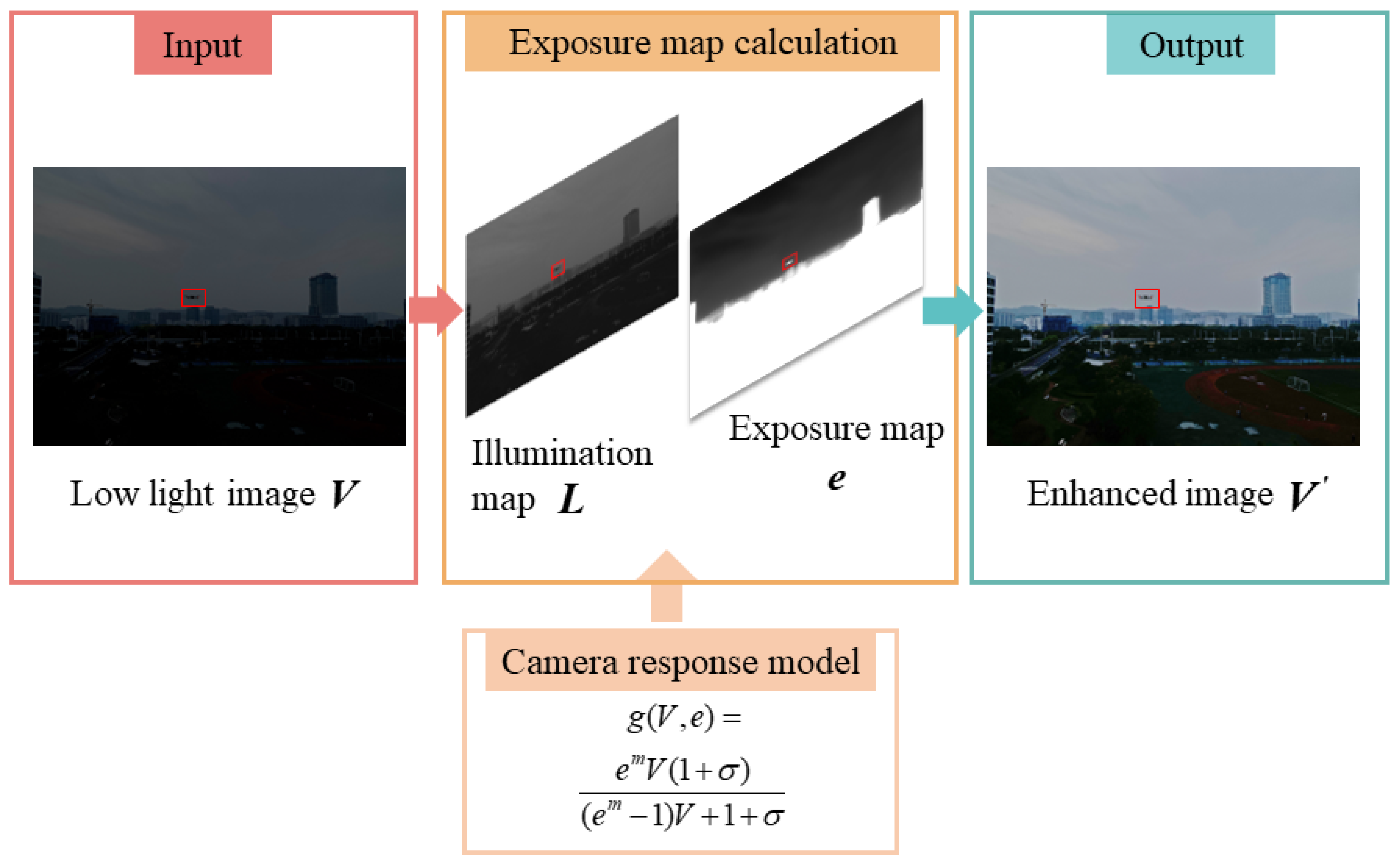
3. The Improved Image Enhancement Algorithm

To address the problem that camera response model-based enhancement algorithms have limited adaptability and can lead to blurred image details, Retinex theory [33] is now introduced to obtain a brightness-enhanced image with sharp details.
Retinex theory decomposes the amount of light reaching the observer into the following two components,
I = R L
where R and L denote the reflectance and light maps of the scene, respectively. The operator ∘ denotes multiplication by an element, and I is the image irradiance representing the amount of light reaching the camera imaging sensor.
Substituting Equation (5) into Equation (1) yields Equation (6), where V denotes the low-light image with image irradiance I mapped to the camera response model.
V = f ( I ) = f ( R L )
The enhanced image V can be expressed as
V = f ( R 1 )
where 1 is an all-1 matrix. Equation (8) is derived from Equations (3) and (5), which gives the relationship between the low-light image V and the enhanced image V .
V = f ( R ) = f ( I ( 1 L ) ) = g ( f ( I ) , 1 L ) = g ( V , 1 L )
The operator ⊘ indicates element-by-element division. According to Equation (8), by adjusting the exposure of the low-light image V , an enhanced image V can be acquired. Therefore, the relationship between the low-light image and the enhanced image can be expressed via Equation (9)
V = g ( V , 1 L ) = g ( V , e )
As large dark areas exist in UAV airborne images under low-illumination conditions, it is important to tailor the image to the actual brightness distribution and make the most appropriate enhancement for each pixel position to avoid significant noise in low SNR areas. Therefore, instead of using a fixed exposure ratio e to enhance the image, we calculate the exposure ratio matrix e of the whole image, which stores the appropriate exposure value for every pixel point in the image.
Thus, in contrast to the fixed exposure ratio e in Equation (2), e in Equation (9) is an exposure value matrix that defines every pixel point’s required exposure value in the image. The exposure ratio matrix e can be derived from Equation (10).
e = 1 L
Equation (9) shows that there are two components of the proposed image brightness enhancement algorithm: (1) selecting an appropriate camera response model and setting the reasonable model parameters; (2) calculating the exposure ratio matrix e to ensure that all pixel positions achieve the required exposure. Equation (10) further shows that the exposure ratio matrix e can be found by calculating L , i.e., the low brightness areas in the UAV airborne image would be adjusted using a high exposure value and the light areas in the UAV airborne image would be adjusted using a low exposure value.

3.1. Camera Response Model Determination

To improve the performance of the proposed algorithm, it is first necessary to determine the mathematical expression for the camera response model f.
This paper uses the two-parameter camera response model Sigmoid, which is based on the human visual system.
f ( I ) = ( 1 + σ ) I m I m + σ
where σ is the weight factor and m is a fixed value of 0.9.
From Equations (1) and (3), the BTF scattering for a specified exposure ratio e can be acquired by Equation (12).
g ( V , e ) = f ( e f 1 ( V ) )
The BTF of Sigmoid can then be computed from Equations (11) and (12).
g ( V , e ) = e m V ( 1 + σ ) ( e m 1 ) V + 1 + σ

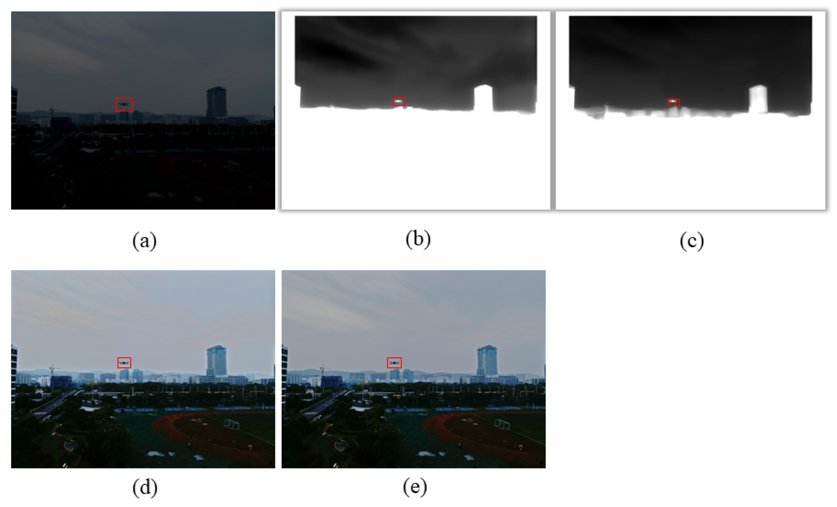
3.2. Exposure Ratio Matrix Calculation

After determining the camera response model, it is further necessary to determine the exposure ratio matrix e . According to Equation (10), e is inversely proportional to the illumination map L . Therefore, L is calculated first and then e is solved by Equation (10). To solve the problem that existing algorithms rely on iterative optimization and calculation time-consuming for calculating illumination map, we adopt the accelerated solver proposed in [20] to solve L . The principle is as follows.
min L L ^ L F 2 + α W L 1
Equation (14) is the objective function for solving the illumination map, where L ^ is the initial illumination map, α is the coefficient used to balance the two terms, and · F and · 1 denote the Frobenius norm and 1 norm, respectively. W is the weight matrix and L is the first order derivative filter. The 1 norm in Equation (14) and the gradient operation on L complicate the process of solving Equation (14), i.e., the presence of the sparse weighted gradient term W L 1 makes the computational process dependent on iterative optimization.
lim ϵ 0 + x d h , v W d x d L x 2 d L x + ϵ = W L 1
where h is the horizontal of pixel x, and v is the vertical of pixel x. Based on Equation (15), approximating W L 1 by x d h , v W d x d L x 2 d L ^ x + ϵ . Then Equation (14) can be written in the following form
min L L ^ L F 2 + α x d h , v W d x d L x 2 d L ^ x + ϵ
Although Equations (14) and (16) are different, we can still extract the illumination map L from the initial illumination map L ^ . This is because if d L ^ x is small then d L x and d L x 2 d L ^ x + ϵ will be inhibited, i.e., because the illumination map L is constrained, no gradient is generated when the initial estimated L ^ exhibits a small gradient. Conversely, when d L ^ x is big, the above inhibition is mitigated as the position is more likely to be on a structural boundary rather than on a regular texture. Equation (16) only involves a quadratic term and can be solved by the following formula
M + d h , v D d T D i a g w ˜ d D d l = l ^
where M is the unit matrix. D consists of D h and D v , which are the Toeplitz matrices deduced from the discrete gradient operators with a forward difference. w ˜ d is the vector form of W ˜ d , W ˜ d x w d x d L ^ x + ϵ . Equation (17) reduces the computational complexity of Equation (14) from O t N log N to O N , where t is the number of iteraions required to converge.
After obtaining the illumination map L , the exposure ratio matrix e is calculated via Equation (10). It is worth noting that setting a high exposure value for a low SNR position will result in a high noise level in a low-light image. Although we can utilize image denoising techniques for noise reduction, it can decrease the efficiency of the enhancement process. As the brightness of UAV vision images is extremely low under low-illumination conditions, this paper sets a maximum exposure value for the extremely low-brightness pixel position to avoid excessive noise in the enhanced image.
e ( x ) = 1 max ( L ( x ) , L min )
where L min is a threshold value. In this paper, we suppose that when the illumination value of a pixel is below L min , the SNR of that pixel is very low and set a maximum exposure value of 1 / L min for it.
Figure 3 shows the effect of setting the maximum exposure value on noise suppression; Figure 3a is a low-illumination image; Figure 3b is the exposure ratio matrix estimated using Equation (10); Figure 3c is the exposure ratio matrix estimated using Equation (18) ( 1 / L min = 1 / 7 ); Figure 3d is the enhanced image by the use of Figure 3b; Figure 3e is the enhanced image by the use of Figure 3c. It can be seen that when the maximum exposure ratio value is not set, the enhanced image becomes noticeably noisy, resulting in a deterioration in image quality. The enhanced image has better visual quality due to less image noise when setting the maximum exposure value, despite the reduced visibility in extremely low-illumination areas.
After calculating the exposure ratio matrix, the low-light image is enhanced using Equation (9). So far, the process of the proposed low-light image enhancement algorithm can be summarized as follows. (1) The low-light image V is inputted, and the camera response model parameter is determined according to the sensor characteristics. (2) To meet the real-time requirements of online processing of airborne images, the accelerated solver in [20] is introduced to obtain the illumination map L corresponding to the low-light image and the exposure ratio matrix e is calculated using Equation (18). (3) Equation (9) is used to enhance the low-light image V to acquire the enhanced image V . Figure 4 visually illustrates the processing flow of the proposed algorithm.

4. Experimental Results and Analysis

4.1. Dataset Construction
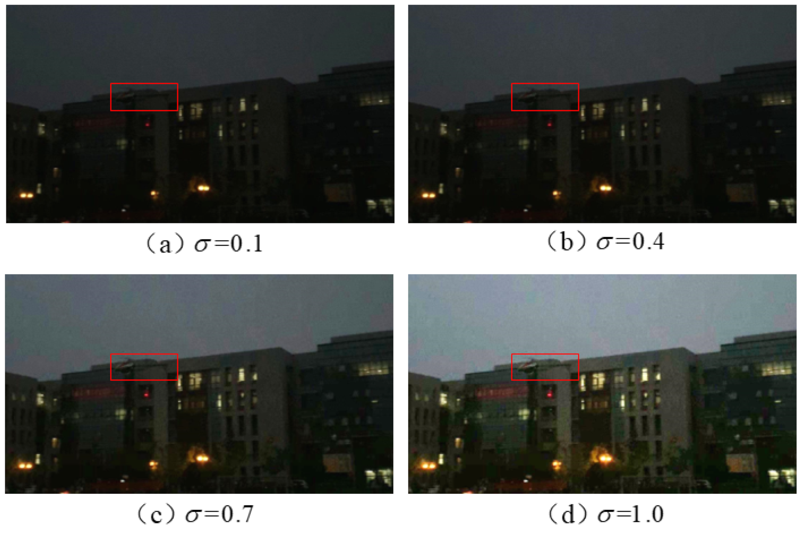
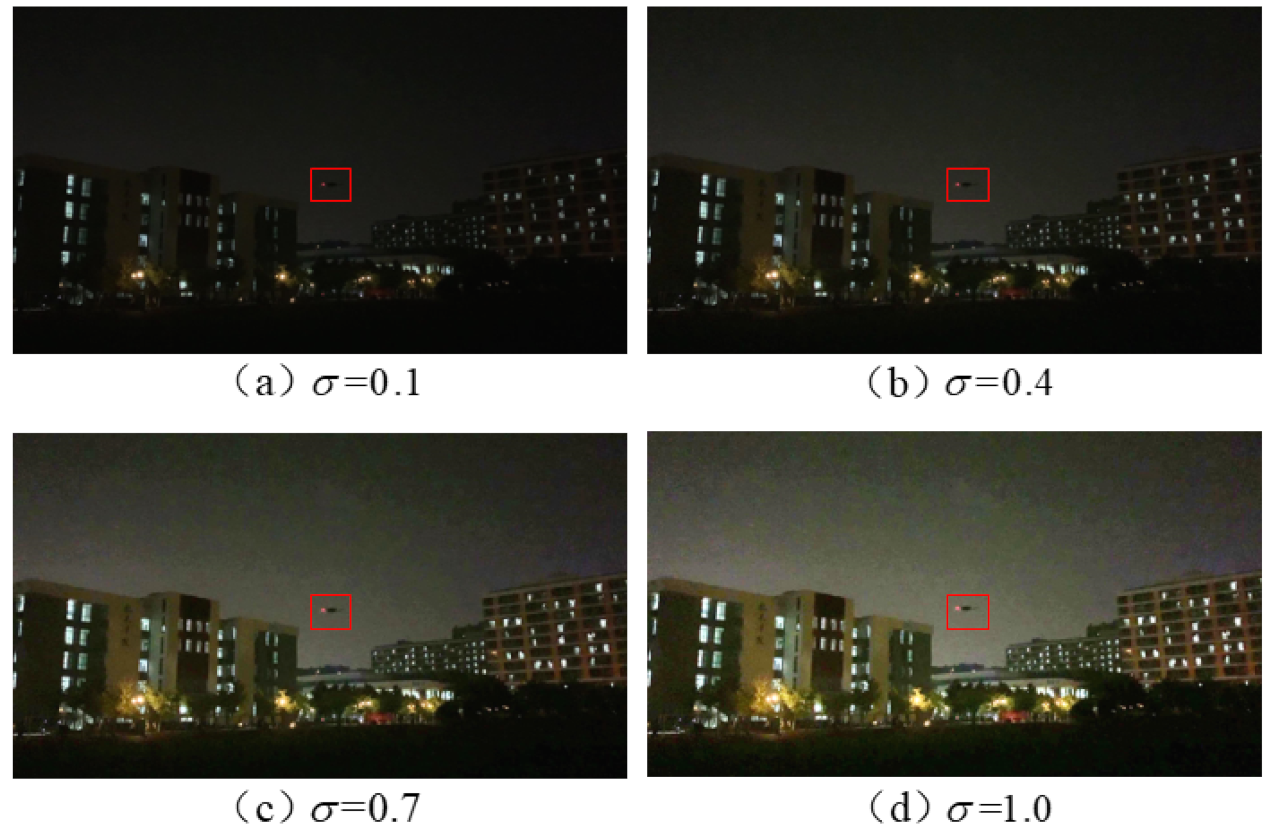
The three types of UAV obstacle objects used to construct the dataset are shown in Figure 5, namely Align 700L V2, DJI F450, and DJI Mavic 2 Pro. The camera properties of another DJI Mavic2 Pro for collecting images are listed in Table 1, and the properties of the three UAV objects are listed in Table 2. For the validation of the proposed algorithm, three video datasets with a resolution of 1920 × 1080 were taken at 6:30 pm (after sunset) on 21 October, in Nanjing University of Aeronautics and Astronautics ( 31 . 940402 N, 118 . 788513 E), Jiangning District, Nanjing, China using another DJI Mavic2 Pro for three types of UAV objects (acting as obstacles), as shown in Figure 6.

4.2. Enhancement When σ Changes

For the proposed algorithm, since the value of the camera model parameters directly determines the effectiveness of the enhancement algorithm, the camera model parameter σ is first analyzed. It is important to note that the optimal values of the model parameters vary with the application scenario, but the general trend of the algorithm effectiveness due to parameter changes is consistent. Therefore, the model parameter specified in this research could be considered to serve as reference values when applying the algorithm to other datasets.
When enhancing the low-light image, the parameter σ of the camera response model Sigmoid affects the effectiveness of the algorithm. Generally, if the parameter σ is too small, the enhancement effect of the low-light image will be insufficient. On the contrary, if σ is too large, the enhancement effect is too strong. However, it may lead to poor effects such as color distortion of the image. In this paper, we set the σ values to increase from 0.1 to 1 in a step of 0.1 to analyze the effect on the enhancement when σ takes different values.
The quantitative evaluation metrics the natural image quality evaluator (NIQE) [34], no-reference free energy based robust metric (NFERM) [35], and information entropy (EN) [36] are used to objectively evaluate the enhancement effect. The smaller the values of the NIQE and NFERM, the better the enhancement. The larger the EN, the more information is retained in the image and the higher quality of the enhanced image.
Figure 7, Figure 8 and Figure 9 show the visualization of the enhancement results of Video 1 containing the Align 700L V2 object, Video 2 containing the DJI F450 object, and Video 3 containing the DJI Mavic 2 Pro object using the proposed algorithm, respectively, when σ is taken to different values. It can be seen from Figure 7, Figure 8 and Figure 9 that the image brightness is improving as the σ gradually increased. The quantitative evaluation results of the enhanced images of Video 1, Video 2, and Video 3 at different σ values using the NIQE, NFERM, and EN are shown in Figure 10, Figure 11 and Figure 12, respectively. From Figure 10, Figure 11 and Figure 12, the NIQE and NFERM decrease as the σ increases, while the EN metric increases. Considering these three objective evaluation indicators and the actual enhanced results comprehensively, the σ was kept constant at 0.8 in this study to achieve good enhanced effects in most cases.

4.3. Comparison Experiments

4.3.1. Time-Consumption Comparison with Similar Brightness Enhancement Algorithms

To validate the superiority of the proposed algorithm in terms of the enhancement process time consumption, the proposed algorithm was compared with several state-of-the-art algorithms, including BIMEF, BPDHE, ENR, MF, and JED. A total of 500 low-light images (1920 × 1080) were selected from the dataset and enhanced using the above algorithms. For fairness, all the experiments were performed in the MATLAB R2020b installed on a desktop equipped with an Intel i7- 9700KF CPU and 32 GB RAM. We find their average processing time for comparison. The time consumption results are shown in Table 3.
From the time consumption results in Table 3, the proposed algorithm has the shortest time consumption and the fastest enhancement speed compared to other algorithms, except for the BIMEF algorithm. This is due to the introduction of an accelerated solver, which compresses the illumination map solution space and reduces the computation amount, thus shortening the time consumption.

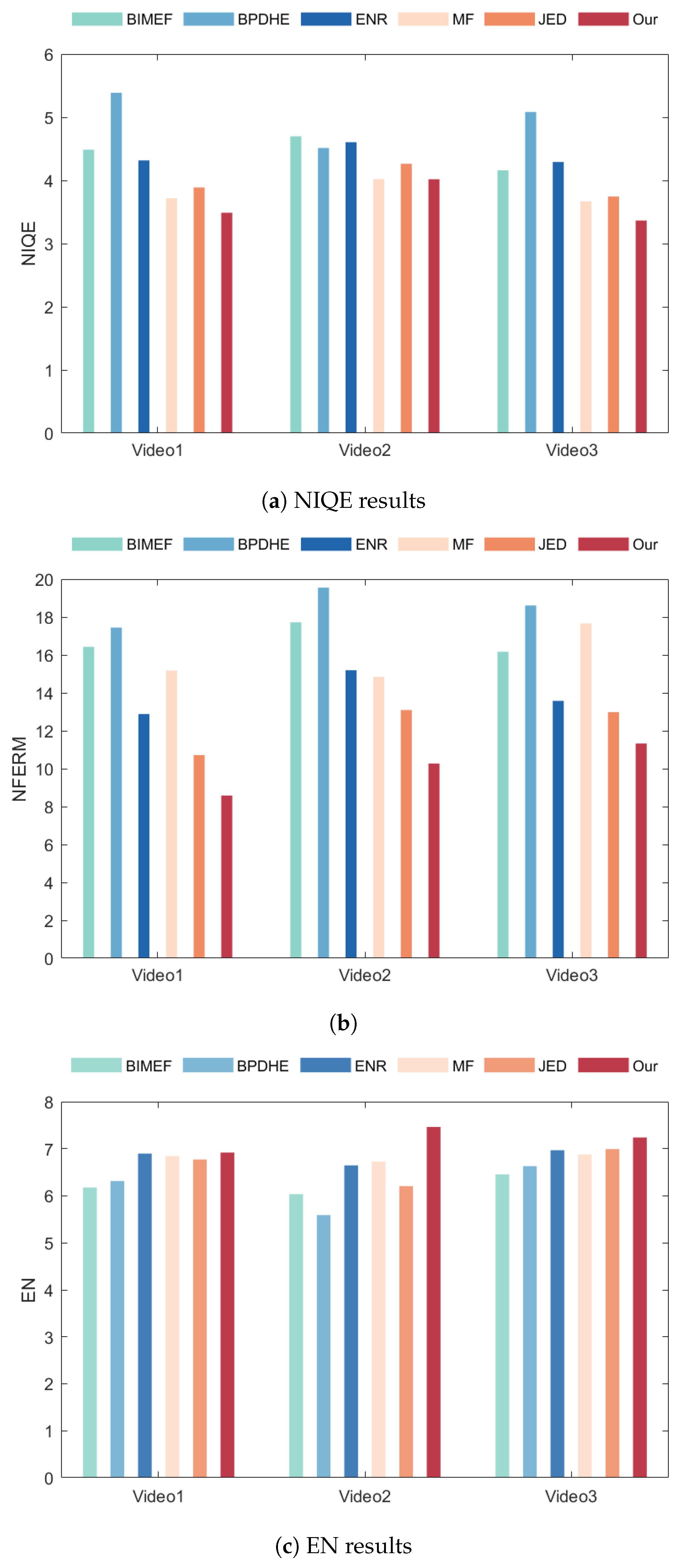
4.3.2. Comparison with Similar Brightness Enhancement Algorithms

To further test the enhancement effect of the proposed algorithm, the proposed algorithm was compared with several state-of-the-art algorithms, including BIMEF, BPDHE, ENR, MF, and JED. Video 1, Video 2, and Video 3 were enhanced by BIMEF, BPDHE, ENR, MF, JED, and the proposed algorithm, respectively. The intuitive enhancement results are shown in Figure 13. Additionally, the quantitative comparison results of the enhanced images using the NIQE, NFERM, and EN metrics are shown in Figure 14.
Figure 13 shows that the brightness enhancement of the BIMEF algorithm is limited. The BPDHE algorithm has a lot of noise in the image. However, the ENR algorithm has a good overall effect, there is some noise in the sky area. In addition, the MF and JED algorithms have too much noise, color distortion, and blurred details in the buildings (shown in the green box). In contrast, the enhanced results of the proposed algorithm have less noise, while retaining more detail and better visual quality of the image. The NIQE and NFERM results of the proposed algorithm in Figure 14a,b are smaller than the compared algorithms, and the proposed algorithm has higher EN results than the other algorithms, as shown in Figure 14c. These quantitative evaluation results show that the proposed algorithm outperforms the compared algorithms in the three metrics of NIQE, NFERM, and EN. Therefore, compared with other algorithms, this algorithm has better enhancement performance.

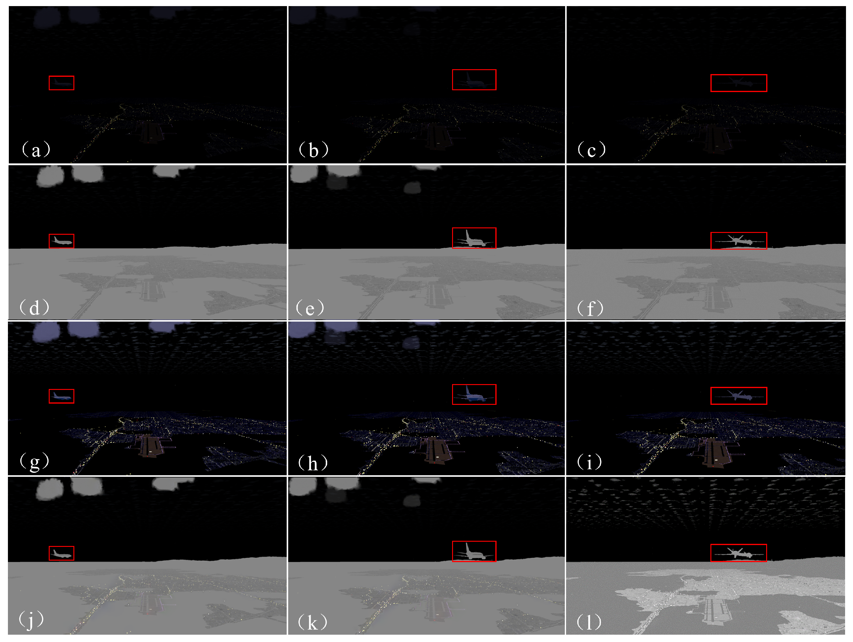
4.3.3. The Effect of Brightness Enhancement on oBstacle Object Detection

The purpose of image enhancement is to raise the detection accuracy of obstacle objects for vision-based obstacle avoidance in low-illumination conditions. Therefore, it is necessary to conduct experiments on obstacle object detection to verify the effectiveness of the proposed low-light image enhancement algorithm. We use YOLO-V3 as the detection model and build a dataset containing UAV obstacle objects to retrain YOLO-V3. The images in the dataset are derived from video streams captured by a Mavic 2 Pro and UAV images from the Internet. For fairness, the training dataset contains images of diverse types of UAVs at different viewing angles, normal light images, low-light images, clear images, and blurred images. The 500 enhanced images containing UAV obstacle objects were used as a test dataset for obstacle detection.
Figure 15 shows the visualization of the obstacle detection results. The number annotated at the top of the yellow frame is the confidence coefficient (Cc) of the obstacle object detection. As can be seen from the first row of Figure 15, the obstacle detection Cc value is low on the original low-light images, and there are cases where the obstacle object is not detected. After being enhanced by BIMEF, BPDHE, ENR, MF, JED, and the proposed algorithm, the detection accuracy is improved and the Cc for obstacle object detection of the enhanced images is all higher than those of the original low-light images. This is shown in rows 2–7 of Figure 15.
For further analysis, the detection average precision (AP) values of the images enhanced by the above enhancement algorithms were calculated, respectively, and those results are summarized in Table 4. The results show that the images enhanced by the proposed algorithm have the highest AP value for obstacle object detection. As can be seen from Figure 15 and Table 4, the proposed enhancement algorithm can improve the accuracy of obstacle detection.

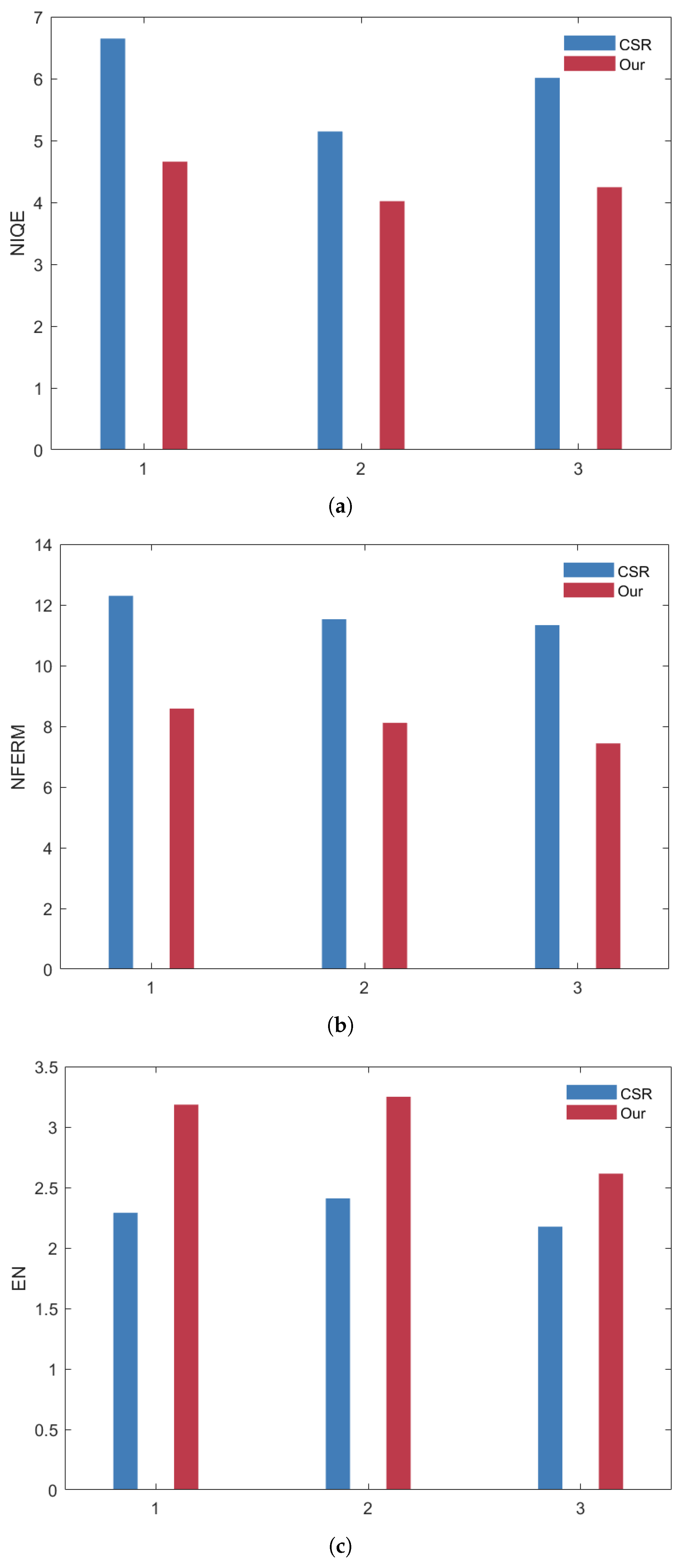
4.3.4. Comparison with the Infrared and Visible Images Fusion Algorithm

To further validate the superiority of the brightness enhancement algorithm based on a single visible image proposed in this paper, it was compared with the infrared and visible images fusion algorithm CSR [37].
To compare the enhancement effect with CSR, three low-light scenarios were created in the FlightGear [38] simulation software, as shown in Figure 16a–c, respectively. Figure 16a is a Boeing 737-300 taken at a distance of 2000 m, Figure 16b is a Boeing 737-300 taken at a distance of 1000 m, and Figure 16c is an MQ-9 taken at a distance of 750 m. The infrared images of the scenes corresponding to Figure 16a–c are Figure 16d–f, respectively, the enhancement results of Figure 16a–c using the proposed algorithm are Figure 16g–i, respectively, and the fusion results of the CSR are shown in Figure 16j–l. From Figure 16g–i, the proposed algorithm can not only effectively improve the image brightness to make the object clearly visible, but also retain the color information to the maximum extent. As shown in Figure 16j–l, although the CSR algorithm can enhance image brightness, the method cannot retain more color information and detail information. The lack of such information will seriously affect the object detection algorithm’s ability to detect and identify the object.
Quantitative evaluation metrics such as NIQE, NFERM, and EN were used to compare and analyze the enhancement results of the proposed algorithm and the CSR algorithm. The results are shown in Figure 17, with horizontal coordinates 1, 2, and 3 indicating the three scenes (a), (b), and (c) in Figure 16, respectively. From Figure 17, the proposed algorithm has better results in three metrics, so the proposed algorithm has better performance than CSR.

5. Conclusions

This paper presents a low-light airborne image enhancement algorithm based on the camera response model and Retinex theory, aiming at the need to overcome the limitations of low-light environments on UAV obstacle avoidance. The contributions of this paper can be summarized as follows.
(1) To address the problem that the existing algorithms can lead to blurred details of the enhanced image, Retinex theory is introduced and combined with the camera response model.
(2) To address the problem that the existing algorithms generate significant noise at low SNR pixel positions during enhancement, the exposure matrix of low-illumination images is obtained by calculating the illumination map, and the maximum exposure ratio value is set for the extremely low SNR pixel position.
(3) The proposed algorithm can increase the AP value of obstacle detection by 0.556 in low-illumination environments, which increases the safety of UAVs flying at night.
However, the proposed algorithm cannot run in real time, GPU parallel acceleration will be considered later as a solution to improve the real-time performance.

Author Contributions

Z.W.: algorithm proposition and testing, data processing, and manuscript writing. D.Z.: research conceptualization, figure design, and manuscript review and editing. Y.C.: directing, project administration, and manuscript review. All authors have read and agreed to the published version of the manuscript.

Funding

This research was funded by the Interdisciplinary Innovation Fund For Doctoral Students of Nanjing University of Aeronautics and Astronautics (No. KXKCXJJ202203) and Postgraduate Research & Practice Innovation Program of Jiangsu Province (No. KYCX20_0210). D.Z. is financially supported by the University of Canterbury, with grant no. 452DISDZ.

Institutional Review Board Statement

Not applicable.

Informed Consent Statement

Not applicable.

Data Availability Statement

The original data have not been made publicly available but can be used for scientific research. Other researchers can send emails to the first author if needed.

Conflicts of Interest

The authors declare no conflict of interest.

References

  1. Peterson, M.; Du, M.; Springle, B.; Black, J. SpaceDrones 2.0—Hardware-in-the-Loop Simulation and Validation for Orbital and Deep Space Computer Vision and Machine Learning Tasking Using Free-Flying Drone Platforms. Aerospace 2022, 9, 254. [Google Scholar] [CrossRef]
  2. Cai, P.; Wang, H.; Huang, H.; Liu, Y.; Liu, M. Vision-based autonomous car racing using deep imitative reinforcement learning. IEEE Robot. Autom. Lett. 2021, 6, 7262–7269. [Google Scholar] [CrossRef]
  3. Tijmons, S.; De Wagter, C.; Remes, B.; De Croon, G. Autonomous door and corridor traversal with a 20-gram flapping wing MAV by onboard stereo vision. Aerospace 2018, 5, 69. [Google Scholar] [CrossRef] [Green Version]
  4. Brukarczyk, B.; Nowak, D.; Kot, P.; Rogalski, T.; Rzucidło, P. Fixed Wing Aircraft Automatic Landing with the Use of a Dedicated Ground Sign System. Aerospace 2021, 8, 167. [Google Scholar] [CrossRef]
  5. Moura, A.; Antunes, J.; Dias, A.; Martins, A.; Almeida, J. Graph-SLAM approach for indoor UAV localization in warehouse logistics applications. In Proceedings of the 2021 IEEE International Conference on Autonomous Robot Systems and Competitions (ICARSC), Santa Maria da Feira, Portugal, 28–29 April 2021. [Google Scholar]
  6. Wang, Z.; Zhao, D.; Cao, Y. Visual Navigation Algorithm for Night Landing of Fixed-Wing Unmanned Aerial Vehicle. Aerospace 2022, 9, 615. [Google Scholar] [CrossRef]
  7. Corraro, F.; Corraro, G.; Cuciniello, G.; Garbarino, L. Unmanned Aircraft Collision Detection and Avoidance for Dealing with Multiple Hazards. Aerospace 2022, 9, 190. [Google Scholar] [CrossRef]
  8. Li, H.; Cao, Y.; Ding, M.; Zhuang, L. Removing dust impact for visual navigation in Mars landing. Adv. Space Res. 2016, 57, 340–354. [Google Scholar] [CrossRef]
  9. González, D.; Patricio, M.A.; Berlanga, A.; Molina, J.M. A super-resolution enhancement of UAV images based on a convolutional neural network for mobile devices. Pers. Ubiquitous Comput. 2022, 26, 1193–1204. [Google Scholar] [CrossRef]
  10. Zhao, L.; Zhang, S.; Zuo, X. Research on Dehazing Algorithm of Single UAV Reconnaissance Image under Different Landforms Based on Retinex. J. Phys. Conf. Ser. 2021, 1846, 012025. [Google Scholar] [CrossRef]
  11. Zhang, K.; Zheng, R.; Ma, S.; Zhang, L. Uav remote sensing image dehazing based on saliency guided two-scaletransmission correction. In Proceedings of the 2021 IEEE International Conference on Image Processing (ICIP), Anchorage, AK, USA, 19–22 September 2021. [Google Scholar]
  12. Wang, W.; Peng, Y.; Cao, G.; Guo, X.; Kwok, N. Low-illumination image enhancement for night-time UAV pedestrian detection. IEEE Trans. Ind. Inform. 2020, 17, 5208–5217. [Google Scholar] [CrossRef]
  13. Gao, T.; Li, K.; Chen, T.; Liu, M.; Mei, S.; Xing, K.; Li, Y.H. A novel UAV sensing image defogging method. IEEE J. Sel. Top. Appl. Earth Obs. Remote Sens. 2020, 13, 2610–2625. [Google Scholar] [CrossRef]
  14. Wu, X.; Liu, X.; Hiramatsu, K.; Kashino, K. Contrast-accumulated histogram equalization for image enhancement. In Proceedings of the 2017 IEEE International Conference on Image Processing (ICIP), Beijing, China, 17–20 September 2017. [Google Scholar]
  15. Ibrahim, H.; Kong, N.S.P. Brightness preserving dynamic histogram equalization for image contrast enhancement. IEEE Trans. Consum. Electron. 2007, 53, 1752–1758. [Google Scholar] [CrossRef]
  16. Lee, C.H.; Shih, J.L.; Lien, C.C.; Han, C.C. Adaptive multiscale retinex for image contrast enhancement. In Proceedings of the 2013 International Conference on Signal-Image Technology & Internet-Based Systems, Kyoto, Japan, 2–5 December 2013. [Google Scholar]
  17. Li, L.; Wang, R.; Wang, W.; Gao, W. A low-light image enhancement method for both denoising and contrast enlarging. In Proceedings of the 2015 IEEE International Conference on Image Processing (ICIP), Quebec City, QC, Canada, 27–30 September 2015. [Google Scholar]
  18. Ying, Z.; Li, G.; Gao, W. A bio-inspired multi-exposure fusion framework for low-light image enhancement. arXiv 2017, arXiv:1711.00591. [Google Scholar]
  19. Ren, X.; Li, M.; Cheng, W.H.; Liu, J. Joint enhancement and denoising method via sequential decomposition. In Proceedings of the 2018 IEEE International Symposium on Circuits and Systems (ISCAS), Florence, Italy, 27–30 May 2018. [Google Scholar]
  20. Guo, X.; Li, Y.; Ling, H. LIME: Low-light image enhancement via illumination map estimation. IEEE Trans. Image Process. 2016, 26, 982–993. [Google Scholar] [CrossRef]
  21. Fu, X.; Zeng, D.; Huang, Y.; Liao, Y.; Ding, X.; Paisley, J. A fusion-based enhancing method for weakly illuminated images. Signal Process. 2016, 129, 82–96. [Google Scholar] [CrossRef]
  22. Li, M.; Liu, J.; Yang, W.; Sun, X.; Guo, Z. Structure-revealing low-light image enhancement via robust retinex model. IEEE Trans. Image Process. 2018, 27, 2828–2841. [Google Scholar] [CrossRef]
  23. Zhu, M.; Pan, P.; Chen, W.; Yang, Y. Eemefn: Low-light image enhancement via edge-enhanced multi-exposure fusion network. In Proceedings of the AAAI Conference on Artificial Intelligence, New York, NY, USA, 7–12 February 2020. [Google Scholar]
  24. Guo, C.; Li, C.; Guo, J.; Loy, C.C.; Hou, J.; Kwong, S.; Cong, R. Zero-reference deep curve estimation for low-light image enhancement. In Proceedings of the IEEE/CVF Conference on Computer Vision and Pattern Recognition, Seattle, WA, USA, 13–19 June 2020. [Google Scholar]
  25. Loh, Y.P.; Chan, C.S. Getting to know low-light images with the exclusively dark dataset. Comput. Vis. Image Underst. 2019, 178, 30–42. [Google Scholar] [CrossRef] [Green Version]
  26. Liu, J.; Duan, M.; Chen, W.B.; Shi, H. Adaptive weighted image fusion algorithm based on NSCT multi-scale decomposition. In Proceedings of the 2020 International Conference on System Science and Engineering (ICSSE), Kagawa, Japan, 31 August–3 September 2020. [Google Scholar]
  27. Hu, P.; Yang, F.; Ji, L.; Li, Z.; Wei, H. An efficient fusion algorithm based on hybrid multiscale decomposition for infrared-visible and multi-type images. Infrared Phys. Technol. 2021, 112, 103601. [Google Scholar] [CrossRef]
  28. Yang, Y.; Zhang, Y.; Huang, S.; Zuo, Y.; Sun, J. Infrared and visible image fusion using visual saliency sparse representation and detail injection model. IEEE Trans. Instrum. Meas. 2020, 70, 1–15. [Google Scholar] [CrossRef]
  29. Nirmalraj, S.; Nagarajan, G. Fusion of visible and infrared image via compressive sensing using convolutional sparse representation. ICT Express 2021, 7, 350–354. [Google Scholar] [CrossRef]
  30. An, W.B.; Wang, H.M. Infrared and visible image fusion with supervised convolutional neural network. Optik 2020, 219, 165120. [Google Scholar] [CrossRef]
  31. Ren, Y.; Yang, J.; Guo, Z.; Zhang, Q.; Cao, H. Ship classification based on attention mechanism and multi-scale convolutional neural network for visible and infrared images. Electronics 2020, 9, 2022. [Google Scholar] [CrossRef]
  32. Mann, S. Comparametric equations with practical applications in quantigraphic image processing. IEEE Trans. Image Process. 2000, 9, 1389–1406. [Google Scholar] [CrossRef] [PubMed] [Green Version]
  33. Land, E.H.; McCann, J.J. Lightness and retinex theory. Josa 1971, 61, 1–11. [Google Scholar] [CrossRef] [PubMed]
  34. Mittal, A.; Soundararajan, R.; Bovik, A.C. Making a “completely blind” image quality analyzer. IEEE Signal Process. Lett. 2012, 20, 209–212. [Google Scholar] [CrossRef]
  35. Gu, K.; Zhai, G.; Yang, X.; Zhang, W. Using free energy principle for blind image quality assessment. IEEE Trans. Multimed. 2014, 17, 50–63. [Google Scholar] [CrossRef]
  36. Roberts, J.W.; Van Aardt, J.A.; Ahmed, F.B. Assessment of image fusion procedures using entropy, image quality, and multispectral classification. J. Appl. Remote Sens. 2008, 2, 023522. [Google Scholar]
  37. Liu, Y.; Chen, X.; Ward, R.K.; Wang, Z.J. Image fusion with convolutional sparse representation. IEEE Signal Process. Lett. 2016, 23, 1882–1886. [Google Scholar] [CrossRef]
  38. Download Link of FightGear 2020.3. Available online: https://www.flightgear.org/ (accessed on 10 June 2022).
Figure 1. Constructure of vision-based obstacle perception and avoidance system.
Aerospace 09 00829 g001
Figure 2. (ad) In one scene, we can get the image pixel V 0 and image pixel V 1 (when setting different exposures) which correspond to irradiance I 0 and irradiance I 1 , respectively.
Aerospace 09 00829 g002
Figure 3. Calculation of exposure ratio matrix.
Aerospace 09 00829 g003
Figure 4. Pipeline of the proposed image enhancement algorithm.
Aerospace 09 00829 g004
Figure 5. The three UAV obstacle objects.
Aerospace 09 00829 g005
Figure 6. Image dataset. Video 1 contains an Align 700L V2 obstacle object, Video 2 contains a DJI F450 obstacle object, and Video 3 contains a DJI Mavic 2 Pro obstacle object.
Aerospace 09 00829 g006
Figure 7. Enhanced results of Video 1 (containing the Align 700L V2 obstacle object) at different σ values.
Aerospace 09 00829 g007
Figure 8. Enhanced results of Video 2 (containing the DJI F450 obstacle object) at different σ values.
Aerospace 09 00829 g008
Figure 9. Enhanced results of Video 3 (containing the DJI Mavic 2 Pro obstacle object) at different σ values.
Aerospace 09 00829 g009
Figure 10. NIQE results for Video 1 (containing the Align 700L V2 obstacle object), Video 2 (containing the DJI F450 obstacle object), and Video 3 (containing the DJI Mavic 2 Pro obstacle object) using the proposed algorithm at different σ values. The lower the NIQE, the better the performance.
Aerospace 09 00829 g010
Figure 11. NFERM results for Video 1 (containing the Align 700L V2 obstacle object), Video 2 (containing the DJI F450 obstacle object), and Video 3 (containing the DJI Mavic 2 Pro obstacle object) using the proposed algorithm at different σ values. The lower the NFERM, the better the performance.
Aerospace 09 00829 g011
Figure 12. EN results for Video 1 (containing the Align 700L V2 obstacle object), Video 2 (containing the DJI F450 obstacle object), and Video 3 (containing the DJI Mavic 2 Pro obstacle object) using the proposed algorithm at different σ values. The higher the EN, the better the performance.
Aerospace 09 00829 g012
Figure 13. Enhancement results of different algorithms for Video 1 (containing the Align 700L V2 obstacle object), Video 2 (containing the DJI F450 obstacle object), and Video 3 (containing the DJI Mavic 2 Pro obstacle object).
Aerospace 09 00829 g013
Figure 14. Quantitative comparisons of the three metrics, i.e., NIQE, NFERM, and EN, on Video 1 (containing the Align 700L V2 obstacle object), Video 2 (containing the DJI F450 obstacle object), and Video 3 (containing the DJI Mavic 2 Pro obstacle object). The six algorithms were selected for comparison. The lower the NIQE and NFERM, the better the performance. The higher the EN, the better the performance. (a) NIQE results. (b) NFERM results. (c) EN results.
Aerospace 09 00829 g014
Figure 15. Obstacle detection results of the images enhanced by different algorithms. The first row is the detection results of the original low-light image, rows 2–7 are the detection results of the BIMEF, BPDHE, ENR, MF, JED, and the proposed algorithm-enhanced images, respectively.
Aerospace 09 00829 g015
Figure 16. Comparison with the CSR algorithm.
Aerospace 09 00829 g016
Figure 17. Quantitative comparison with CSR algorithm. The lower the NIQE and NFERM, the better the performance. The higher the EN, the better the performance. (a) NIQE results. (b) NFERM results. (c) EN results.
Aerospace 09 00829 g017
Table 1. Camera properties of the other DJI Mavic 2 Pro.
UAVImage SensorPixelsFOVApertureISO RangeShutter SpeedVideo Resolution
DJI Mavic 2 Pro1 inch CMOS20 MP77 f/2.8– f/11100–64008–1/8000 s1920 × 1080
Table 2. Properties of the three UAV obstacle objects.
UAVAlign 700L V2DJI F450DJI Mavic 2 Pro
Dimensions1320 × 220 × 360 mm450 × 450 × 350 mm322 × 242 × 84 mm
Weight5100 g1357 g907 g
Table 3. Comparison of time consumption of the six algorithms.
AlgorithmBIMEFBPDHEENRMFJEDOurs
Mean time consumption (s)0.531.992.963.944.110.88
Table 4. The AP results of the images enhanced by different algorithms.
ImageLow-Light ImageBIMEFBPDHEENRMFJEDOur
AP0.3010.5720.5070.7400.7860.7490.857
Publisher’s Note: MDPI stays neutral with regard to jurisdictional claims in published maps and institutional affiliations.

