GIS-Based Spatial Patterns Analysis of Airspace Resource Availability in China

Abstract

Identifying the factors influencing airspace resources, quantifying the availability of airspace resources, and mastering their spatial distribution characteristics are the cornerstone of scientific and efficient airspace management. Therefore, this paper investigates the impact of prohibited, restricted, and dangerous areas (PRDs) on airspace resource availability from a traffic flow perspective, proposes a multi-layer network model, and establishes a flow-based sector resource availability (FSRA) calculation model. The FSRA in mainland China is calculated above the standard pressure altitude of 6000 m. The results show that the FSRA is lower when the sector is determined to have a higher PRD density, a more complex traffic flow pattern, and a more sophisticated interaction between the two. China’s mainland airspace is separated into three altitude ranges along the vertical direction according to the FSRA and sector distribution: 6000–7800 m, 7800–8900 m, and 8900–12,500 m. The spatial distribution characteristics of the FSRA are addressed using the ArcGIS software. The results demonstrate that spatial autocorrelation is exhibited for all three altitude ranges. The high–high cluster pattern mainly occurs in the western part of mainland Chinese airspace, while the low–low cluster pattern is distributed in the southeast. The three altitude ranges are divided into three groups, respectively, and suggestions for airspace management are made for each group.

1. Introduction

Airspace resources refer to the airspace elements that are capable of meeting the current or future needs of mankind, generating use value and affecting labor productivity in air transportation production [1]. As passengers pursue economic and convenient air travel, global air transport activities are on the rise, which leads to the further aggravation of the contradiction between constrained airspace resources and growing air traffic demand, decreased airspace operation efficiency, increased flight delays, and even crises related to civil aviation safety [2]. Therefore, there is an urgent need for scientific and effective airspace management to achieve efficient use of airspace resources, in order to boost aviation traffic and decrease delays [3].

According to the ICAO, Air Traffic Management (ATM) consists of three components: Air Traffic Service (ATS), Airspace Management (ASM), and Air Traffic Flow Management (ATFM). ASM aims to achieve full utilization of airspace in accordance with established airspace conditions and, to the extent possible, to meet the needs of all parties using the airspace [4]. The Federal Aviation Administration (FAA) has studied the new concept of dynamic and flexible airspace management, and noted that in the strategic, pre-tactical, and tactical three-level airspace coordination mechanism, different airspace management measures are adopted in stages to alleviate the conflict between air traffic flow demand and limited airspace resources [5]. Based on ASM, Eurocontrol proposed the airspace management concept of Flexible Use of Airspace (FUA) to accomplish airspace allocation and flexibility through the establishment of flexible airspace structures and procedures, such as conditional routes, temporary segregated areas, and temporary reserved areas [6]. Then the concept of Advanced Flexible Use of Airspace (AFUA) is studied to improve airspace support capability by airspace sharing [7].

It is obvious that scientific ASM technologies can improve airspace resource availability. However, the relevant factors affecting the airspace resource availability are not yet clear. Moreover, few studies evaluate the availability of civil airspace resources, and most focus on terminal areas [8,9], with scant evidence for studies that cover an entire nation or region. Even more infrequent are the findings from research on the spatial distribution characteristics of civil airspace resources.

With this in mind, this paper investigates the impact of prohibited, restricted, and dangerous areas (PRDs) on airspace resource availability from the perspective of traffic flow, and establishes a more scientific, objective, and systematic method of calculating the availability of civil airspace resources on this basis. GIS technology is introduced to innovatively investigate the distribution patterns of airspace resource availability. It contributes to capturing the impact of PRDs and traffic flow on airspace resources, assists airspace users in having a more comprehensive and intuitive grasp of the availability and distribution of civil airspace resources, facilitates the rational planning and the use of civil airspace resources, and provides new ideas and methods for scientific and efficient ASM.

The rest of this paper is organized as follows. Section 2 summarizes the relevant literature on the research methods covered in this paper. Section 3 describes the methodology of this paper. Section 3.1 introduces the data preprocessing and the establishment of control sector metadata. Section 3.2 presents the “structure-flow” multi-layer network model. Section 3.3 proposes a flow-based sector resource availability calculation model. Section 3.4 and Section 3.5 introduce spatial autocorrelation analysis and spatial grouping analysis methods, respectively. Section 4 carries out a case study of the airspace in mainland China to quantify the airspace resource availability while fulfilling the resource demands of existing airspace users, and thoroughly examines the spatial patterns and spatial correlations of airspace resource availability. Finally, some conclusions and future research directions are provided in Section 5.

2. Related Work

2.1. Evaluation Method of Airspace Resource Availability

Nowadays, there are relatively few studies quantifying airspace resource availability. Most of the current research results start with the key index of airspace utilization, that is, an evaluation model of airspace utilization is constructed from different perspectives, and the utilization of airspace resources is then recognized. On the basis of the ratio of the actual arriving and departing flights to the arrival and departure capacity of the terminal area, MITRE [10] defined the arrival utilization, departure utilization rate, and the mixed arrival and departure utilization to evaluate the utilization of airport resources. Wanke et al. [11] evaluated the sector utilization according to the ratio of air traffic flow within the sector in a 15 min time slice to the Monitor Alert Parameter (MAP) issued by the FAA. Based on MAP, Michael et al. [12] assessed multi-sector airspace utilization by counting the number of sector hours exceeding MAP in the multi-sector airspace. In the design of airspace tube structures, Sheth et al. [13] presented instantaneous occupancy and volume occupancy to address the spatiotemporal utilization of airspace tube structures. Following the space-time map in ground transportation, Min [14] analyzed the utilization of corridors-in-the-sky temporally and spatially. Li et al. [15] developed an evaluation index system of the utilization rate in the terminal area from multiple dimensions and estimated the grade of the daily utilization rate in the terminal area by using a comprehensive evaluation method. In the study of low-altitude airspace resources, Qiu et al. [16] built a low-altitude airspace resource availability evaluation index system and employed regression analysis to derive the utilization of low-altitude airspace resources.

Several research results have completed the metrics of airspace resources by building mathematical models. With the airport serving as the core and the entrance and exit points and the key waypoints of the terminal area as its elements, Shi et al. [17] developed a model to evaluate residual civil aviation airspace resources. Based on this model, the residual airspace resources were quantified by calculating the traffic at the elements. According to the BeiDou grid location code technology system, Shu et al. [18] converted the civil aviation airspace elements into a 3D spatial grid model and developed a calculation method of the 3D spatial grid model to calculate the airspace resources.

In conclusion, the establishment of an airspace utilization evaluation model can be broadly split into two parts: on the one hand, a model has been constructed according to the actual operation process from the viewpoints of flow, time, and space, among others; on the other hand, it is based on an evaluation index system to assess the airspace utilization. The majority of the airspace resource calculation methods that are in use are based on the flow of elements through the airspace or on the distribution of airspace elements. However, the aforementioned assessment methods do not take into account the relationship between air transport demand and airspace resources, nor do they consider the impact of the distribution relationship between airspace elements such as sectors and PRDs on the availability of airspace resources, making it challenging to use for a thorough evaluation of civil airspace resource availability.

2.2. Trajectory Clustering

Trajectory clustering is the process of dividing the trajectory dataset into several similar object classes, which ensures that the similarity between trajectories within a class is maximized and that the similarity between classes is minimized [19]. It is applied to the field of air traffic to identify the spatial and temporal distribution of air traffic flow from massive trajectory data. Among them, traditional clustering algorithms such as K-means, Density-Based Spatial Clustering of Applications with Noise (DBSCAN), and spectral clustering are widely used in trajectory clustering. Barratt et al. [20] adopted the K-means algorithm to complete track clustering and identified the center trajectory, based on which aircraft trajectory prediction was accomplished. Zhong et al. [21] fulfilled trajectory reconstruction based on a characteristic point of the trajectory and applied K-means to determine the flight status in the terminal area. Chu et al. [22] employed K-means as the basis cluster and obtained the clustering results. According to multiple clustering results, the similarity matrix was constructed, and the hierarchical clustering algorithm was utilized to achieve trajectory clustering in the terminal area airspace. Wang et al. optimized DBSCAN by introducing the local outlier factor (LOF), which improved the clustering effect by eliminating outliers [23]. Corrado et al. [24] established a weighted Euclidean distance function to measure the similarity between trajectories and then used Hierarchical DBSCAN (HDBSCAN) to cluster the trajectories in the terminal area. The results showed that this method could enhance the clustering effect. Spectral clustering originated from graph theory and was later used in track clustering. Xiao et al. [25] introduced a method for calculating the distance between trajectories and set up a distance matrix; then, the spectral clustering algorithm was utilized to cluster the trajectories. In order to cluster the trajectories more objectively, Sun et al. [26] determined the number of clusters based on the silhouette coefficient and used the spectral clustering algorithm to cluster the air traffic trajectories in the terminal area.

With the unceasing development of deep learning technology, some experts and scholars use deep learning methods for trajectory clustering. Olive et al. [27] implemented trajectory clustering using deep convolutional embedded clustering (DCEC) and artifact techniques with autoencoders. Zeng et al. [28] developed a trajectory clustering method based on a combination of the deep autoencoder (DAE) and Gaussian mixture model (GMM) to identify the traffic flow patterns in the terminal airspace.

Nowadays, methods related to trajectory clustering have been developed and are more mature, but different clustering algorithms have their own strengths and shortcomings: the traditional clustering algorithm is easy to implement, but the randomness is strong. Clustering algorithms based on deep learning have higher clustering accuracy with less memory, but they need to fit a large number of hyperparameters. The choice of clustering algorithm still depends on specific cases. Most of the existing research results are focused on the airport terminal area, and there is less research related to clustering flight trajectories in the control sector and distinguishing the traffic flow patterns.

2.3. GIS-Based Spatial Analysis

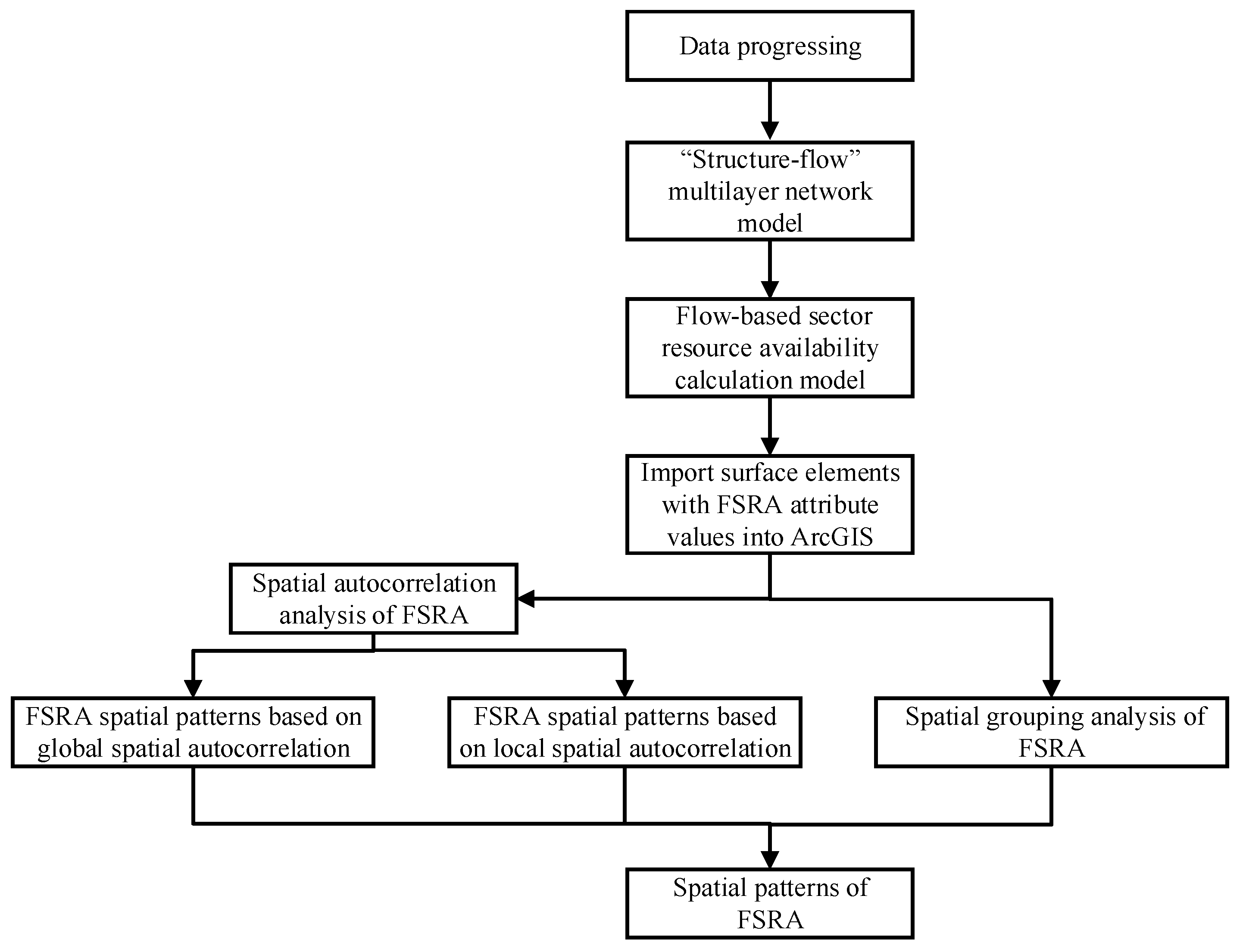
Since geospatial issues are involved in the location of airspace sectors, practically all spatial data are spatially interrelated [29]. As a result, the use of traditional statistical analysis methods to analyze airspace resource availability cannot characterize this spatial correlation well. GIS technology not only has robust spatial mapping and spatial visualization capabilities, which can help us to have a more visual and intuitive understanding of the distribution of the object under study, but it also has powerful spatial analysis and data management functions, which can be employed to examine the spatial distribution characteristics of the object under study from a variety of angles [30]. GIS technology is currently being extensively applied in many different fields to mine the spatial distribution features of objects. In terms of the spatial distribution of traffic accidents, Ulak et al. [31] suggested a GIS-based spatial analysis method to identify high-risk crash locations based on the clustering of crashes on a roadway network and then compared the geospatial differences of traffic crashes between aging drivers and crashes involving other age groups. Lu et al. [32] investigated the peculiarities of the spatial distribution of road traffic accidents in Shenzhen using density analysis and spatial cluster analysis techniques in GIS. In the study of Wang et al. [33], the spatial distribution of marine accidents in terms of accident frequency and severity was examined using density analysis and cluster analysis. In the spatial distribution of pollution, Khalil et al. [34] examined the spatial distribution of pollutants in abandoned mine sites and predicted the mine pollution that had occurred using GIS technology in conjunction with a database. Based on the existing AirGIS, Jibran et al. [35] developed a new modeling system that is the new AirGIS to explore the spatial distribution features of ambient air pollution. From the perspective of the spatial distribution of natural disasters, Jiang et al. [36] conducted a quantitative study on the relationships between rocky desertification and the spatial patterns of land use in the Nandong underground river system, a typical karst area, in Southwest China. Majumder et al. [37] employed Moran’s I to evaluate the spatial autocorrelation of floods in the Bongaon sadar sub-division and the Getis-OrdGi*(d) to identify regions that can be considered hotspots and cool spots for floods. With the aid of Google Earth imageries and field visits, Naseer et al. [38] determined the spatial distribution of landslides in the District Neelum of Pakistan, then produced distribution maps using the Digital Elevation Model and ArcGIS and analyzed its feature classes. In the field of disease spatial distribution, Wang et al. [39] visualized the specifics of COVID-19 in China using the ArcGIS software to correlate COVID-19 data with a vector map of administrative regions in China and obtained the spatial distribution characteristics of COVID-19 in China using spatial autocorrelation analysis and hotspot analysis methods. Cahyadi et al. [40] adopted the weighted mean center, directional distribution, Getis-Ord Gi *, Moran’s I, and spatially weighted regression to investigate the spatiotemporal distribution and transmission patterns of COVID-19 in Surabaya.

Some researchers have recently included GIS in their research on airspace. On the basis of GIS, Scaini et al. [41] analyzed the effects of volcanic ash diffusion on air traffic parameters (airports, routes, and airspace sectors) following volcanic eruptions. Oktal et al. [42] examined the volume of traffic in Turkish airspace above FL 245 using GIS. Li et al. [43] produced a linear density distribution map of regional aircraft flight trajectories using trajectory data and the density analysis method in GIS technology.

The above-mentioned research findings show that despite the widespread use of GIS technology in other fields, relatively little research has been carried out on its application to research in the airspace, and no pertinent research on the spatial distribution characteristics of civil airspace resource availability has been conducted.

3. Methodology

In this study, the basic information on airspace structure and aircraft trajectory were obtained from National Aeronautical Information Publication (NAIP) and ADS-B data, respectively. Since this study calculated civil resource availability in terms of sectors, it was necessary to discretize the above data. In order to analyze the impact of PRDs on airspace resources under traffic flow, a “structure-flow” multi-layer network model was established from the perspective of “static sector structure-dynamic traffic flow distribution”. To estimate the civil resource availability of sectors, a flow-based sector resource availability (FSRA) calculation model was subsequently put forth. Finally, the sectors of various altitude ranges were created as surface elements with attribute values for the FSRA and were imported into ArcGIS for spatial analysis: global spatial autocorrelation was used to represent the spatial characteristics of the FSRA in the airspace of mainland China, and local spatial autocorrelation was used to identify high–low clustering and outliers in local airspace, to describe the spatial distribution characteristics of the FSRA more comprehensively. The airspace was grouped using the spatial grouping analysis method for several groups, and the associated airspace resource allocation and optimization methods were then developed. Figure 1 provides an illustration of the structure for the suggested framework.

3.1. Data Processing

This study explored the resource availability of control sectors above the standard pressure altitude of 6000 m. The airspace structure data were obtained from the 2019 NAIP, excluding Hong Kong, Taiwan, and Macao, with 223 control sectors, and a total of 268 PRDs. Figure 2 depicts the distribution of the control sectors and PRDs in the airspace of mainland China as well as the positional relationship between the control sectors and PRDs. It also depicts the relationship between China’s national boundaries and the mainland airspace. The aircraft trajectories were from Chinese flight trajectory data taken in November 2019. As can be observed, the eastern airspace of China has a small sector size but a high sector density, several PRDs, and a convoluted distribution and location of airspace features. The pattern of airspace resource strain will worsen due to China’s rising demand for air traffic. In contrast, the western region of China has a sizable airspace area with few PRDs and a generally straightforward aviation environment.

The data above need to be discretized because the resource availability in this research was computed in terms of sectors. The metadata needed for calculating the resource availability of each sector are displayed in

Table 1. Metadata of control sector.

Metadata	Property Description
Sector boundary points	Latitude and longitude coordinates constituting sector boundaries
Sector altitude	The altitude range of the sector, including minimum and maximum altitude
PRD boundary points	Latitude and longitude coordinates constituting PRD boundaries
PRD altitude	The altitude range of PRDs, including minimum and maximum altitude
Flight trajectories	All ADS-B trajectories in the sector
Flow distribution	Latitude and longitude coordinates of the flow
Traffic volume	Number of aircraft on the flow
Interaction	Interaction among flow, PRDs, and sector boundaries

.

The distribution of PRDs in the sector may differ at various altitude ranges, as may the distribution of flow. Additionally, there are high and low sector phenomena. As a result, the relative positional relationship between traffic flow, PRDs, and sector boundaries is complicated.

3.2. “Structure-Flow” Multi-Layer Network Model

In the sector-based operation, from a static point of view, the delimitation of the PRDs and the location relationship between the PRDs and the sector will occupy airspace resources; from the dynamic point of view, the use of airspace resources will be influenced by the operation of the aircraft and the relationship between their positions, and the non-linear interaction between the distribution of the airspace elements and the aircraft’s operation in the sector will also affect airspace resource usage. Therefore, from the standpoint of “static sector structure-dynamic traffic flow distribution,” a novel analysis framework based on multi-layer networks was developed. It consists of a Flight Trajectory Network (FTN), a Traffic Flow Network (TFN), and a Flow-based Sector Resource Availability Network (FSRAN). Figure 3 depicts these networks, which are further elaborated in the individual sections below. Among them, the PRDs are illustrated by P1, P2, and P3 in the sector structure of Figure 3.

3.2.1. Flight Trajectory Network (FTN)

The FTN is made up of flight trajectory data obtained following data preprocessing and using resampling technology, based on the flight trajectories provided by the ADS-B monitoring equipment. The network provides crucial information for the creation of the TFN and encapsulates the temporal–spatial distribution of air traffic in the sector unit.

A flight trajectory is a multi-dimensional time series composed of a set of vertices that are unevenly distributed, and each vertex represents one ADS-B snapshot of a single flight. Therefore, the trajectory sample set U, trajectory FP, and vertex p are constructed for each sector. The datasets are as follows:

$$U={\{FP}_1,F{P}_2,\cdots ,F{P}_i,\cdots ,F{P}_n\}$$

(1)

$$F{P}_i={\{\mathit{p}}_{i1},{\mathit{p}}_{i2},\cdots ,{\mathit{p}}_{ij},\cdots ,{\mathit{p}}_{im}\}$$

(2)

$${\mathit{p}}_{ij}={\{t}_{ij},x_{ij},y_{ij},z_{ij},s_{ij},v_{ij},{\theta }_{ij}\}$$

(3)

where U is the set of all flight trajectories in the sector; n is the total number of flight trajectories in the sector; and $F{P}_i$ represents the i-th flight trajectory, where $i\in \left[1,n\right]$. Each trajectory includes multiple vertices sorted by a timestamp; m represents the number of vertices that form the trajectory; and the j-th vertex of i-th flight trajectory is ${\mathit{p}}_{ij}$, where $j\in \left[1,m\right]$. ${\mathit{p}}_{ij}$ comprises seven elements that represent the timestamp, longitude, latitude, altitude, speed, vertical speed, and heading. It is worth noting that the vertical speed is almost equal to 0 when the aircraft is flying along a certain flight level.

Owing to the large scale of the flight trajectory data, direct computation will lead to low computational efficiency, and the number of vertices may not be the same for various trajectories. In the cruise flight phase, for maximum fuel efficiency, the aircraft strives to avoid changes in speed and height, so its flight parameters, such as heading and speed, essentially remain unchanged. As a result, the trajectory data are resampled to logically reduce the size of the data while preserving the flight characteristics of the aircraft. The uniform parameterization method is used to resample the trajectory data, and the trajectory $F{P}_i$ is parameterized to [0, 1] using the cumulative chord length in Equation (4) as a parameter:

$$\begin{array}{l}{u}_{i1}=0\\ u_{ij}=u_{i(j-1)}+\frac{\sqrt{{\left(x_{ij}-x_{i(j-1)}\right)}^2+{\left(y_{ij}-y_{i(j-1)}\right)}^2+{\left(z_{ij}-z_{i(j-1)}\right)}^2}}{{\displaystyle \sum _{j=2}^m\sqrt{{\left(x_{ij}-x_{i(j-1)}\right)}^2+{\left(y_{ij}-y_{i(j-1)}\right)}^2+{\left(z_{ij}-z_{i(j-1)}\right)}^2}}}\end{array}\}$$

(4)

where $u_{ij}$ represents the parameter value corresponding to the j-th vertex in the trajectory $F{P}_i$, $u_{i1}=0$, $u_{im}=1$. The initial and last vertices are left intact after parameterization, and the parameter node $\frac{l-1}{q-1}\left(l=1,2,\cdots ,q-1\right)$ is determined as the resampling point based on the resampling point number q. The flight track after resampling is: $F{P}_i{}^{\prime }=\{{\mathit{p}}_{i1}{}^{\prime },{\mathit{p}}_{i2}{}^{\prime },\cdots ,{\mathit{p}}_{il}{}^{\prime },\cdots ,{\mathit{p}}_{iq}{}^{\prime }\}$, where ${\mathit{p}}_{i1}{}^{\prime }={\mathit{p}}_{i1}$, ${\mathit{p}}_{iq}{}^{\prime }={\mathit{p}}_{im}$. The flight trajectory sample set after resampling is $U^{\prime }={\{FP}_1{}^{\prime },F{P}_2{}^{\prime },\cdots ,F{P}_i{}^{\prime },\cdots ,F{P}_n{}^{\prime }\}$, which constitutes the FTN.

3.2.2. Traffic Flow Network (TFN)

According to trajectory clustering, the FTN is developed for sector-based operation. The FTN is utilized to create a similarity matrix based on the weighted Euclidean distance, and spectral clustering is then used to finish the flight trajectory clustering. Finally, the TFN is built using the mean value method to determine the traffic flow distribution situation. Since all of the flight trajectories in the TFN have an identical number of vertices, the inter-trajectory distance calculation can be completed by a vertex pair for any two trajectories $F{P}_i{}^{\prime }$ and $F{P}_j{}^{\prime }$ in $U^{\prime }$. The similarity of the trajectories in the TFN is estimated based on the trajectory variables of longitude, latitude, altitude, speed, vertical speed, and heading using the Weighted Euclidean distance (WED) approach. The WED can be calculated as follows:

$$\mathrm{WED}\left(F{P}_i{}^{\prime },F{P}_j{}^{\prime }\right)={\displaystyle \sum _{l=1}^q\left({\omega }_1\mathrm{dist}(u_{il},u_{jl})+{\omega }_2\mathrm{dist}({\theta }_{il},{\theta }_{jl})+{\omega }_3\mathrm{dist}(s_{il},s_{jl})+{\omega }_4\mathrm{dist}(v_{il},v_{jl})\right)}$$

(5)

where $\mathrm{dist}(u_{il},u_{jl})$, $\mathrm{dist}({\theta }_{il},{\theta }_{jl})$, $\mathrm{dist}(s_{il},s_{jl})$, and $\mathrm{dist}(v_{il},v_{jl})$ in Equation (5) stand for the Euclidean distance of position, heading, speed, and vertical speed between each vertex pair, respectively, and ${\omega }_i>0(i=1,2,3,4)$ is the corresponding weight for each Euclidean distance and ${\displaystyle \sum _{i=1}^4{\omega }_i=1}$. This study takes ${\omega }_1=0.6$, ${\omega }_2=0.2$, ${\omega }_3=0.1$, and ${\omega }_4=0.1$. The similarity between the two trajectories increases as the $\mathrm{WED}\left(F{P}_i{}^{\prime },F{P}_j{}^{\prime }\right)$ becomes smaller. In order to further reduce errors and to improve the computing efficiency, $\mathrm{WED}\left(F{P}_i{}^{\prime },F{P}_j{}^{\prime }\right)$ is standardized by Equation (6), where $\max \left\{\mathit{A}\right\}$ and $\min \left\{\mathit{A}\right\}$ are the maximum WED and the minimum WED between trajectories, respectively. Finally, the similarity matrix is obtained as shown in Equation (7):

$$a_{ij}=\frac{\mathrm{WED}\left(F{P}_i{}^{\prime },F{P}_j{}^{\prime }\right)-\min \left\{\mathit{A}\right\}}{\max \left\{\mathit{A}\right\}-\min \left\{\mathit{A}\right\}}$$

(6)

$$\mathit{A}=\left[\begin{array}{cccc}0& a_{12}& \cdots & \begin{array}{ccc}{a}_{1i}& \cdots & a_{1n}\end{array}\\ a_{21}& 0& \cdots & \begin{array}{ccc}{a}_{2i}& \cdots & a_{2n}\end{array}\\ ⋮& ⋮& \ddots & \begin{array}{ccc}⋮& \ddots & ⋮\end{array}\\ \begin{array}{c}{a}_{i1}\\ ⋮\\ a_{n1}\end{array}& \begin{array}{c}{a}_{i2}\\ ⋮\\ a_{n2}\end{array}& \begin{array}{c}\cdots \\ \ddots \\ \cdots \end{array}& \begin{array}{ccc}\begin{array}{c}0\\ ⋮\\ a_{ni}\end{array}& \begin{array}{c}\cdots \\ \ddots \\ \cdots \end{array}& \begin{array}{c}{a}_{in}\\ ⋮\\ 0\end{array}\end{array}\end{array}\right]$$

(7)

Most clustering algorithms require one or more input parameters, and the clustering quality is significantly influenced by the input parameters. Spectral clustering has strong adaptability to the data structure distribution and can guarantee convergence to the global optimal solution. Spectrum clustering merely requires the parameter of the “clustering number” to be determined, and the clustering effect is typically better than the other classic clustering techniques [44]. As a result, spectral clustering is chosen to complete trajectory clustering.

Following the completion of clustering, the mean value method is used to obtain the center track for each clustering result. This center track characterizes the traffic flow. Then, it aggregates all of the traffic flows to create a TFN. The whole process of the TFN establishment based on spectral clustering is shown in Algorithm 1.

Algorithm 1. TFN based on spectral clustering

Input: Similarity matrix A Output: TFN 1. Build the Degree matrix D which is a diagonal matrix where $d_{ii}={\displaystyle \sum _{j=1}^n{a}_{ij}}$ (8);

2. Build the Laplace matrix L of A: $\mathit{L}={\mathit{D}}^{-1}\left(\mathit{D}-\mathit{A}\right){\mathit{D}}^{-1}$ (9);

3. Calculate the eigenvalues of L and sort them from large to small, and then extract the eigenvectors corresponding to the first k eigenvalues: ${\mathit{v}}_1,{\mathit{v}}_2,\cdots ,{\mathit{v}}_k$;

4. Build the eigenvector matrix ${\mathit{V}}_{n\times k}=\left[{\mathit{v}}_1,{\mathit{v}}_2,\cdots ,{\mathit{v}}_k\right]$ and normalize it to generate matrix Z;

5. Cluster the Z based on the K-means algorithm, the number of clusters is k;

6. Use the mean value method to extract the center track for each clustering result;

7. The TFN is constructed by assembling all the center tracks;

8. end

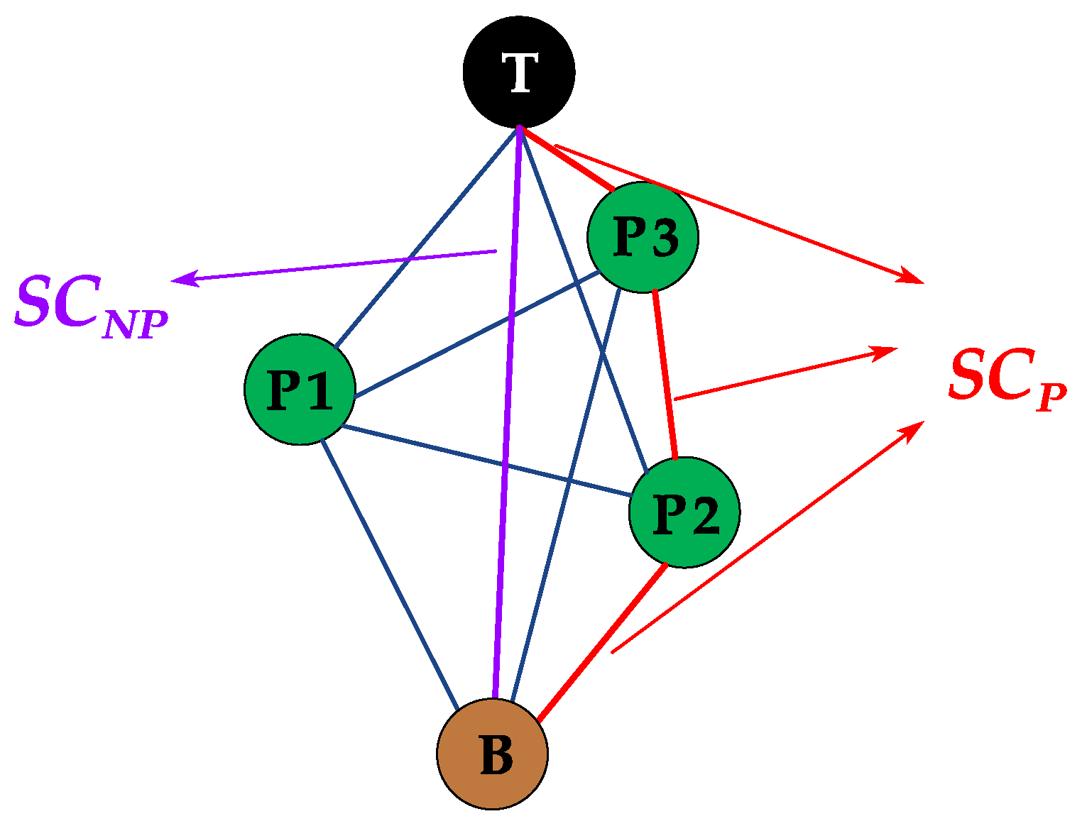
3.2.3. Flow-Based Sector Resource Availability Network (FSRAN)

When PRDs are present, aircrafts can still be guided in the portion of the airspace sector that is not covered by PRDs. Thus, the FSRA is defined as follows: under a certain traffic flow organization, the ratio of sector capacity in the presence of PRDs (SC_P) to that in the absence of PRDs (SC_NP) in the airspace sector, and this ratio can indicate the extent of sector resource availability, and the FSRA is calculated according to Equation (8). The FSRAN is thus developed using information about the sector structure and the TFN.

$$FSRA=\frac{S{C}_P}{S{C}_{NP}}$$

(10)

(1)

Sector model abstraction

The sector is abstracted as a two-dimensional polygonal region, and the traffic flow and PRDs at various flight levels are taken into account. To facilitate the subsequent establishment of the sector model, the following simplified assumptions are made:

• All aircrafts cannot pass through PRDs.
• Aircrafts are not permitted to generate or terminate within the sector, and all aircrafts must enter or exit from the boundaries of the sector.
• The research scope is a single flight level, i.e., the aircraft will not change altitude in the sector, and cannot climb or descend within the sector boundary.
• Aircrafts can approach PRDs at will as long as they do not enter them.
• When an aircraft enters and exits from two neighboring boundaries, an “L”-shaped angle constraint with a length of 5 km is set with the safety viewpoint [45]. In Figure 4, A–D are the pinch angle constraints, and “bottleneck” cells are also depicted when aircrafts are flying in and out from different directions.

(2)

Construction of FSRAN

The max-flow min-cut theorem is a classical theorem and method in network flow theory, according to which in a network flow, the capacity of a min-cut is equal to the value of a max-flow. Thus, the value of the max-flow of a network depends on the bottleneck cell capacity of the network. Strang [46] extended the max-flow min-cut theorem for discrete networks to 2D polygonal domains, and Gewali et al. [47] argued that the cut capacity is proportional to the distance between the polygon boundary and the obstacles.

A polygonal sector is shown in Figure 5, and P1, P2, and P3 represent the PRDs within the sector. Based on the direction of traffic flow, the polygon sector boundary is divided into source edge (s), sink edge (t), top edge (T), and bottom edge (B). Among them, the entry and exit edges of traffic flow are s and t, respectively. On the left side of the traffic flow, all edges other than s and t make up T, while on the right side, all edges other than s and t make up B. The blue dashed line in Figure 5 indicates the minimum Euclidean distance between the polygonal sector boundary and the PRDs. Therefore, the min-cut of the polygon sector under traffic flow can be expressed by the minimum distance from T to B, and the value of max-flow through the polygon sector is equal to the min-cut capacity.

The above 2D polygonal sector is abstracted into a network, which is defined as the FSRAN, as shown in Figure 6. A pair of vertices in the FSRAN are connected by an edge whose length is equal to the minimum (Euclidean) distance between the PRDs that correspond to the vertices. Then, the shortest path problem between T and B is resolved using Dijkstra’s algorithm. The min-cut made in the polygonal sector by the traffic flow is the length of the shortest path, which represents the sector capacity in the presence of PRDs, i.e., SC_P. The minimum distance between T and B represents the sector capacity in the absence of PRDs, which is SC_NP. The final FSRA is obtained according to Equation (10).

3.3. Flow-Based Sector Resource Availability Calculation Model

Based on the “structure-flow” multi-layer network model, this study suggests a flow-based sector resource availability calculation model to quantitatively explain the sector resource availability. The model takes into account both the static sector structure and the traffic flow distribution with dynamic characteristics, allowing it to comprehensively and precisely assess the FSRA.

Since each traffic flow in the TFN is able to enter and exit through different boundaries of the airspace sector, there are variations in the FSRA that correspond to various traffic flow distributions. Therefore, this paper innovatively focuses on how the TFN’s traffic flow directly affects the FSRA calculation. The traffic flow is weighted according to the traffic volume on each traffic flow, and finally, the FSRA of the sector covered by the TFN is determined. Considering that the PRD distribution and TFN of the same sector may differ in each altitude range, the FSRA of the sector in each altitude range should be calculated independently. The whole calculation process of the FSRA is shown in Algorithm 2, and the relevant parameters are described in

Table 2. Parameter symbol description.

Parameter	Implication
F	Set of all the flows in TFN, $F=\left\{1,2,\dots ,n\right\}$.
P	Set of all the PRDs in sector structure, $P=\left\{1,2,\dots ,e\right\}$.
f	Flow index, $f\in F$.
h	PRD index, $h\in P$.
$X_f$	Set of all the elements in FSRAN under flow f, $f\in F$.
$R_f^{\mathrm{T}}$	Top edge under flow f, $f\in F$.
$R_f^{\mathrm{B}}$	Bottom edge under flow f, $f\in F$.
$S{C}_{P,f}$	Min-cut with PRDs under flow f, $f\in F$.
$S{C}_{NP,f}$	Min-cut without PRDs under flow f, $f\in F$.
$FSR{A}_f$	FSRA under flow f, $f\in F$.
$Q_f$	The number of aircraft on the flow f, $f\in F$.
${\eta }_f$	Weight of flow f, $f\in F$.
$d(p,q)$	Shortest Euclidean distance between p and q.

.

Algorithm 2. The whole FSRA calculation process

Input: TFN, Sector Structure, FSRAN

Output: FSRA

1. for $f=1,2,\cdots ,n$ do

2. $X_f=\left\{R_f^{\mathrm{T}},P_1,P_2,\cdots ,P_h,R_f^{\mathrm{B}}\right\}$

3. ${\mathit{Y}}_f=d{(p,q)}_{(e+2)\times (e+2)}=\left[\begin{array}{cccc}0& d(R_f^{\mathrm{T}},P_1)& d(R_f^{\mathrm{T}},P_2)& \begin{array}{ccc}\cdots & d(R_f^{\mathrm{T}},P_h)& d(R_f^{\mathrm{T}},R_f^{\mathrm{B}})\end{array}\\ d(P_1,R_f^{\mathrm{T}})& 0& d(P_1,P_2)& \begin{array}{ccc}\cdots & d(P_1,P_h)& d(P_1,R_f^{\mathrm{B}})\end{array}\\ d(P_2,R_f^{\mathrm{T}})& d(P_2,P_1)& 0& \begin{array}{ccc}\cdots & d(P_2,P_h)& d(P_2,R_f^{\mathrm{B}})\end{array}\\ \begin{array}{c}⋮\\ d(P_h,R_f^{\mathrm{T}})\\ d(R_f^{\mathrm{B}},R_f^{\mathrm{T}})\end{array}& \begin{array}{c}⋮\\ d(P_h,P_1)\\ d(R_f^{\mathrm{B}},P_1)\end{array}& \begin{array}{c}\ddots \\ \cdots \\ \cdots \end{array}& \begin{array}{c}\begin{array}{ccc}\ddots & ⋮& ⋮\end{array}\\ \begin{array}{ccc}d(P_h,P_{h-1})& 0& d(P_h,R_f^{\mathrm{B}})\end{array}\\ \begin{array}{ccc}d(R_f^{\mathrm{B}},P_{h-1})& d(R_f^{\mathrm{B}},P_h)& 0\end{array}\end{array}\end{array}\right]$(11)

4. Calculate the shortest path $S{C}_{P,f}$ of ${\mathit{Y}}_f$ using the Dijkstra algorithm which is the min-cut with PRDs;

5. Calculate shortest path $S{C}_{NP,f}$ of ${\mathit{Y}}_f$ which is the min-cut without PRDs:

$S{C}_{NP,f}=d(R_f^{\mathrm{T}},R_f^{\mathrm{B}})$                     (12)

6. Calculate the FSRA for flow f: $FSR{A}_f=\frac{S{C}_{P,f}}{S{C}_{NP,f}}$         (13)

7. Calculate the weight corresponding to flow f: ${\eta }_f=\frac{Q_f}{{\displaystyle \sum _{f=1}^n{Q}_f}}$     (14)

8. Calculate the FSRA of a sector: $FSRA={\displaystyle \sum _{f=1}^n{\eta }_f\times }FSR{A}_f$    (15)

9. end for

3.4. Spatial Autocorrelation Analysis

Based on statistics, spatial autocorrelation analysis is used to examine the potential dependence of the spatial variables with a certain regularity in space at different spatial locations [48]. Moran’s I and G index are the primary indices for gauging the severity of dependence. Meanwhile, the combination of global spatial autocorrelation analysis and local spatial autocorrelation analysis is heavily applied to various spatial problems [49]. Therefore, this paper selects global spatial autocorrelation and local spatial autocorrelation analysis methods and employs Moran’s I as the spatial autocorrelation coefficient to quantify the degree of spatial interdependence of the FSRA.

3.4.1. Global Spatial Autocorrelation Analysis

Global spatial autocorrelation analysis is utilized to identify the spatial pattern of the region as a whole and to determine whether there is an aggregation of an attribute feature in the overall spatial scope. The spatial autocorrelation of the FSRA is tested using Moran’s I, which is calculated as shown in Equations (16) and (17).

$$I=\frac{n{\displaystyle \sum _{i=1}^n{\displaystyle \sum _{j=1}^n{W}_{ij}\left(x_i-\overline{x}\right)\left(x_j-\overline{x}\right)}}}{{\displaystyle \sum _{i=1}^n{\left(x_i-\overline{x}\right)}^2{\displaystyle \sum _{i=1}^n{\displaystyle \sum _{j=1}^n{W}_{ij}}}}}$$

(16)

$$\overline{x}=\frac{1}{n}{\displaystyle \sum _{i=1}^n{x}_i}$$

(17)

where I is Moran’s I, and n is the number of sectors involved in the analysis. $x_i$ and $x_j$ denote the FSRA of sector i and sector j, respectively, where $i\ne j$. $W_{ij}$ is the spatial weight matrix, and the inverse distance method is utilized to generate the spatial weight matrix between sectors, i.e., the closer the distance, the greater the possibility of interaction between sectors. $\overline{x}$ represents the mean value of the FSRA.

The values of Moran’s I vacillate from −1 to +1; a positive value for Moran’s I indicates that a sector with high FSRA values has an adjoining sector with an equally high FSRA value. An adverse value for Moran’s I indicates that a sector has neighboring sectors with low FSRA values. Since Moran’s I does not have a significance test function, it was converted into a normal test statistic Z to test for significance concerning a normal distribution table, which is calculated as Equation (18).

$$Z\left(I\right)=\frac{I-E\left(I\right)}{\sqrt{\mathrm{Var}\left(I\right)}}$$

(18)

where E(I) and Var(I) are the expected value and variance of Moran’s I, respectively.

3.4.2. Local Spatial Autocorrelation Analysis

Local spatial autocorrelation analysis is employed to determine the correlation degree of attribute feature values between the reference space unit and its neighboring space unit. In this study, the Local Indications of Spatial Association (LISA) agglomeration graph was utilized to identify the high-value and low-value clusters and outliers of the FSRA in the local spatial sectors. For a specific sector, the LISA equation for Moran’s I is as follows:

$$I_i=\frac{n\left(x_i-\overline{x}\right){\displaystyle \sum _{j=1}^n{W}_{ij}\left(x_j-\overline{x}\right)}}{{\displaystyle \sum _{i=1}^n{\left(x_i-\overline{x}\right)}^2}}$$

(19)

The parameters in Equation (19) are the same as in Equations (16) and (17). If the local spatial autocorrelation is significant, it indicates that there is a certain degree of spatial correlation or spatial difference between the FSRA of this sector and its surrounding sectors, and the specific spatial relationship contains four types: clusters of sectors with high FSRA values (high–high), clusters of sectors with low FSRA values (low–low), outliers in which sectors with high FSRA values are primarily surrounded by sectors with low FSRA values (high–low), and outliers in which sectors with low FSRA values are primarily surrounded by sectors with high FSRA values (low–high).

3.5. Spatial Grouping Analysis

Spatial cluster analysis is one of the key techniques for identifying geographical patterns and carrying out spatial mining, and the primary distinction between spatial clustering analysis and traditional clustering analysis is the introduction of spatial relationships. In addition to taking object attribute values into account, spatial clustering also considers spatial proximity. This study exploits the grouping analysis tool in ArcGIS10.7 which was created by the Environmental Systems Research Institute Inc (Esri), founded in 1969 and headquartered in Redlands, California, USA, to perform spatial clustering analysis by considering the spatial location proximity of the sector and the FSRA attribute information.

The grouping analysis tool adopts unsupervised machine learning procedures to determine natural clusters in the data based on the specified number of groups, and it then provides a solution that makes the elements inside each group as similar as possible while remaining distinct from one another [50]. CONTIGUITY_EDGES_CORNERS is selected as the space constraint parameter, which indicates that the topological relationship between the surface elements (sectors) can be grouped only when the boundary or nodes are shared. Then, a minimum-span tree that can reflect both the spatial organization of the surface elements and their attribute values is established. The Spatial “K” Cluster Analysis by the Tree Edge Removal (SKATER) method is used to iteratively remove the branches of the tree. Finally, the spatial clustering results of the specified number of groups are generated. The evaluation parameter of the grouping analysis effect is R², and a larger R² signifies a better element differentiation. The equations are as follows.

$$R^2=\frac{\mathrm{SST}-\mathrm{SSE}}{\mathrm{SST}}$$

(20)

$$\mathrm{SST}={{\displaystyle \sum _{i=1}^{b_c}{\displaystyle \sum _{j=1}^{b_i}{\displaystyle \sum _{k=1}^{b_w}\left(V_{ij}^k-\overline{V^k}\right)}}}}^2$$

(21)

$$\mathrm{SSE}={{\displaystyle \sum _{i=1}^{b_c}{\displaystyle \sum _{j=1}^{b_i}{\displaystyle \sum _{k=1}^{b_w}\left(V_{ij}^k-\overline{V_i^k}\right)}}}}^2$$

(22)

where b represents the number of elements (i.e., number of sectors); $b_c$ represents the number of classes (number of groups); $b_i$ represents the number of elements in group i; $b_w$ is the number of variables (only consider the FSRA, $b_w=1$) used for element grouping; $V_{ij}^k$ is the k-th variable value of the element j in group i; $\overline{V^k}$ is the average value of variable k; and $\overline{V_i^k}$ is the average value of variable k in group i.

4. Results

4.1. FSRA Calculation of an Example Sector

Taking the control sector ZSSSAR25 as an example, the FSRA of the sector was calculated. According to the available metadata, the altitude range of ZSSSAR25 is 7800–12,500 m, but there are variations in the PRDs of this sector at various altitude ranges. Figure 7 depicts the “structure-flow” multi-layer network model for various altitude ranges based on the content in Section 3.2.

To compute the FSRA, the longitude and latitude coordinates corresponding to the sector boundary points, PRD boundary points, and traffic flow distribution were first converted to rectangular plane coordinates by the Mercator projection method. Additionally, the FSRA of control sector ZSSSAR25 was determined based on Algorithm 2. The calculation results are shown in

Table 3. FSRA calculation results in the altitude range of 7800–8900 m.

Parameter of FSRA	Value
$Q_{1,1}$	7108
$Q_{1,2}$	1792
${\eta }_{1,1}$	0.799
${\eta }_{1,2}$	0.201
${\mathrm{FSRA}}_{1,1}$ ${\mathrm{FSRA}}_{1,2}$	0.736
	0.939
${\mathrm{FSRA}}_1$	0.777

and

Table 4. FSRA calculation results in the altitude range of 8900–12,500 m.

Parameter of FSRA	Value
$Q_{2,3}$	6668
$Q_{2,4}$	7156
$Q_{2,5}$	1768
${\eta }_{2,3}$	0.428
${\eta }_{2,4}$	0.459
${\eta }_{2,5}$	0.113
${\mathrm{FSRA}}_{2,3}$	1
${\mathrm{FSRA}}_{2,4}$	1
${\mathrm{FSRA}}_{2,5}$	0.939
${\mathrm{FSRA}}_2$	0.993

.

4.2. FSRA Spatial Patterns in Chinese Airspace

Based on the above research method, the FSRA of the control sectors above the standard pressure altitude of 6000 m was quantified. Combining the sector distribution, sector altitude situation, and FSRA value, the airspace of mainland China is divided into three ranges along the altitude direction: 6000–7800 m, 7800–8900 m and 8900–12,500 m. Some sector distributions and FSRA values were different at various altitude ranges. Figure 8 shows the spatial distribution of the FSRA in the airspace of mainland China. The names of the sectors were recorded from a confidentiality perspective. From an overall perspective, the FSRA of mainland China’s airspace shows obvious agglomeration distribution characteristics. The southeasterly airspace is a typical low-value agglomeration area: political, economic, and cultural development have led to a high volume of air traffic flow in the eastern airspace, but the eastern airspace has a limited sector size and a high density of PRDs, which results in a low FSRA. The FSRA of A2, M2, S27, S13, and S32 are the lowest among them and do not exceed 0.25. When combined with the real scenario, it is clear that the aforementioned sectors, which have a high density of PRDs, have more intricate interactions between traffic flow and PRDs, resulting in a reduction in the sector resource availability. The western airspace belongs to the high-value aggregation area and has a large sector size, few PRDs, little air traffic, and abundant available resources in the airspace, and the FSRA is larger than 0.7.

4.3. Spatial Autocorrelation Analysis of FSRA

The sectors of various altitude ranges were converted into area features containing the FSRA attribute values, and the spatial statistics function of ArcGIS10.7 software was used to conduct the spatial autocorrelation analysis of the FSRA in Chinese airspace.

4.3.1. FSRA Spatial Patterns Based on Global Spatial Autocorrelation

The global Moran’s I statistics were obtained to determine the FSRA area features at different altitude ranges, and the calculated values are shown in

Table 5. Global Moran’s I statistics of FSRA at different altitude ranges.

Altitude Ranges	Moran’s I	Z Score	p Value
6000–7800 m	0.113458	3.293467	0.000990
7800–8900 m	0.089418	2.637853	0.008343
8900–12,500 m	0.087378	2.585902	0.009712

.

It can be seen from Table 5 that the Z scores for the various altitude ranges are all greater than the critical value of 2.58 with 1% significance, indicating that the FSRA distribution is only less than 0.001 likely to be randomly distributed, and the possibility of an aggregated distribution is significantly higher than the possibility of a random distribution. Additionally, Moran’s I is positive, suggesting that the spatial distribution of the FSRA in the airspace of mainland China is aggregated and has a spatially positive correlation pattern. In other words, sectors with a higher (lower) FSRA are spatially adjacent to one another. There is an overall spatial dependence, with 6000–7800 m being the strongest, 7800–8900 m being the next strongest, and 8900–12,500 being the weakest.

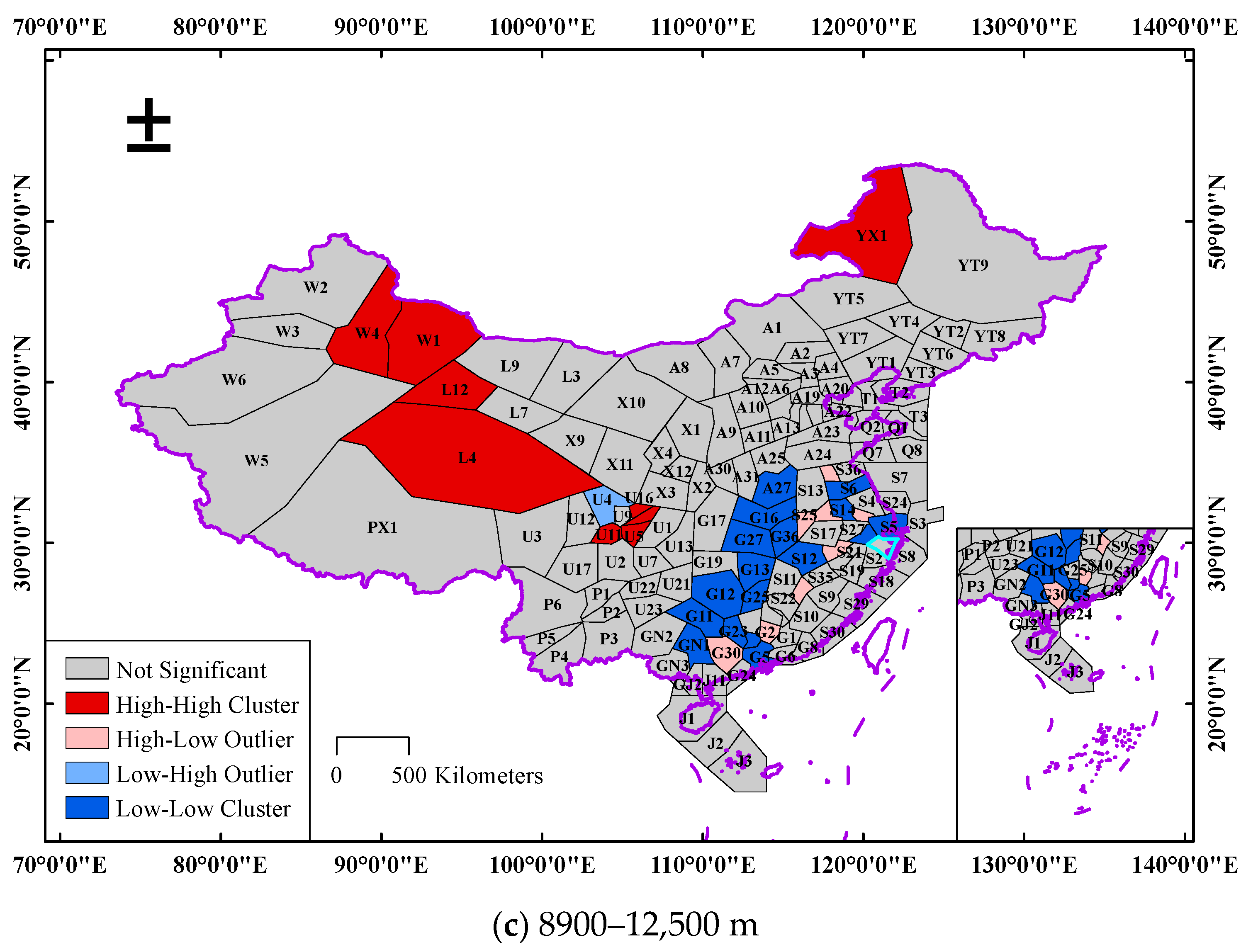
4.3.2. FSRA Spatial Patterns Based on Local Spatial Autocorrelation

Global spatial autocorrelation analysis can only reflect the spatial relationship of the FSRA in the whole airspace but cannot reveal the distribution characteristics of the FSRA in local airspace. Therefore, this paper employs local spatial autocorrelation for further analysis, and the LISA agglomeration graph of the FSRA at different altitude ranges is shown in Figure 9.

The outcomes of the local spatial autocorrelation analysis of the FSRA in the three altitude ranges are comparable from a global perspective. The sectors including W1, W4, L4, L12, U11, U15, and U16 are located in the western part of the airspace of mainland China and present a high–high cluster pattern in all three altitude ranges, which demonstrates that the above sectors have a greater degree of civil airspace resource availability. YX1 and J3 also exhibit a high–high cluster pattern, for they have no PRDs or small PRDs with the FSRA equal to 1. The low–low clusters are all located in the southeastern part of the China mainland airspace, and their corresponding areas include cities such as Beijing, Shanghai, Guangzhou, among others. These cities hold developed economic, political, cultural, and tourism industries, and have large airports such as Shanghai Pudong International Airport, Beijing Daxing International Airport, and Beijing Capital International Airport, which absorb a large amount of air traffic flow. However, for air defense and other needs, a large quantity of PRDs are set up in the corresponding airspace of the above-mentioned areas, so the civil airspace resources that are available are scarce.

The low–high outliers are distributed in the southeastern part of the airspace of China. Their distribution is relatively scattered, and most of them are spread around the low–low clusters. The FSRA value of these sectors corresponding to the low–high outliers is high due to the area of the PRDs in the above sectors being smaller, or the interaction between the PRDs and traffic flow being smaller. The high–low outlier is found in sector U4, which is adjacent to the sectors with high FSRA values, but there are large areas of PRDs in U4, so the FSRA value of this sector is lower.

Owing to the distinctions in sector distribution and the values of the FSRA in various altitude ranges, the results of local spatial autocorrelation analysis in different altitude ranges are not identical. The difference is the greatest in the altitude range from 6000 to 7800 m. The sectors M1, M2, M3, M4, GH1, GH2, GH3, and GH4 are defined in the southeast of the Chinese airspace at this altitude range, which varies from the sectors established in the remaining two altitude ranges (see Figure 9). The FSRA values for the above sectors are small, where the FSRA of the M2 is only 0.17287, so the low–low clusters in this altitude range are notably different.

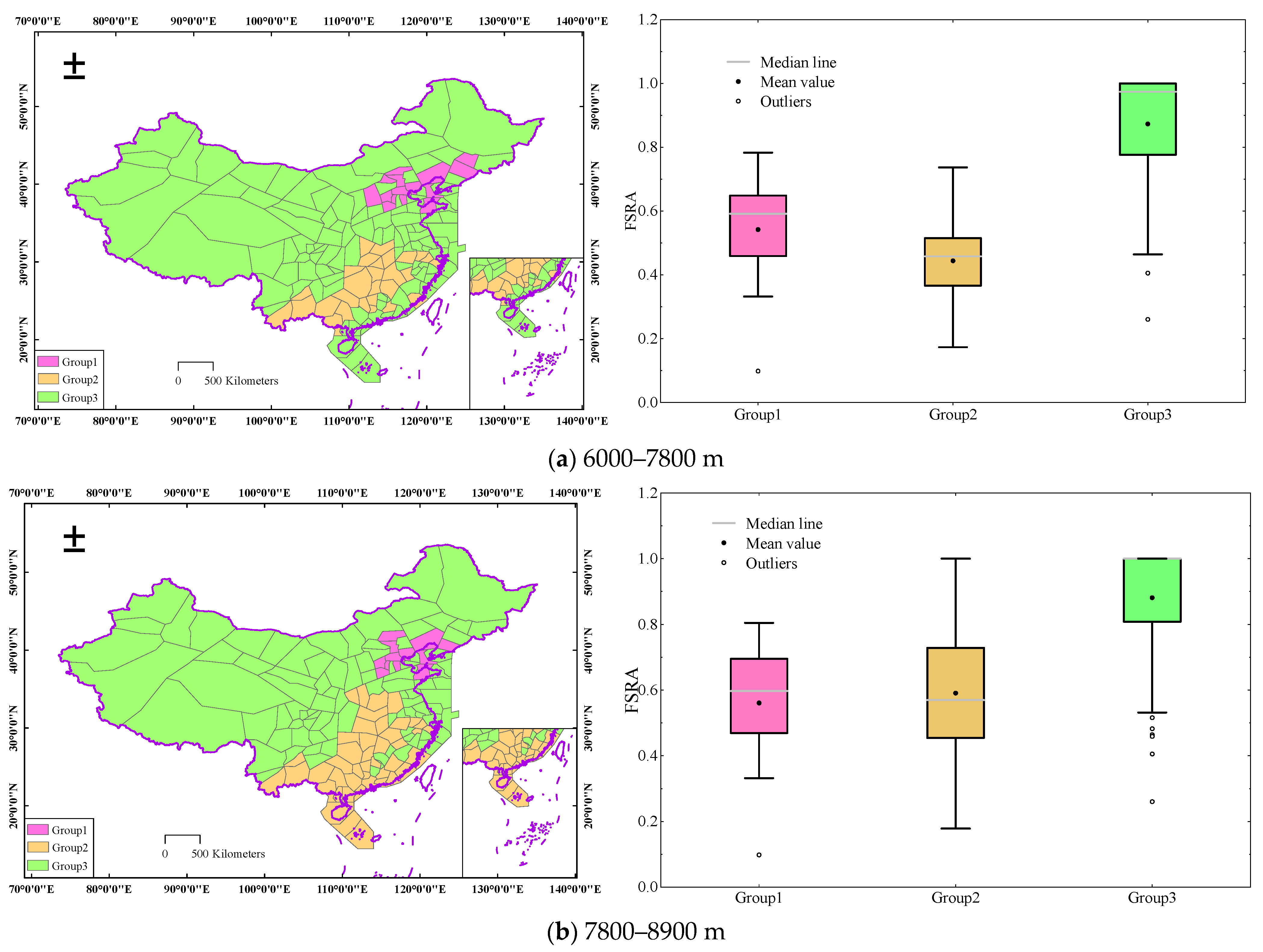
4.4. Spatial Grouping Analysis of FSRA

It is evident from the above analytical results that the FSRA has a regional agglomeration effect in the airspace of mainland China. Based on this, a spatial clustering analysis of the FSRA for Chinese airspace was performed at various altitude ranges. In this paper, three groups were created after taking into account the actual situation and the number of better groups.

Table 6. Grouping analysis results of FSRA in Chinese airspace.

Altitude Ranges	R2
6000–7800 m	0.7141
7800–8900 m	0.6926
8900–12,500 m	0.6679

displays the grouping outcomes for various altitude ranges. Table 6 shows that the R² in the altitude range from 6000 to 7800 m reaches 0.7141, indicating that this altitude range has the best grouping effect. Therefore, the spatial clustering results are shown in Figure 10 when the number of groups is three and the spatial constraint relationship is indicated by CONTIGUITY _ EDGES _ CORNERS.

Figure 10 shows that while the spatial distribution of the clustering results at various altitude ranges seems similar, the FSRA values in each group at various altitude ranges are unique. In the altitude range from 6000 to 7800 m, Group1 corresponded to the second lowest FSRA value, with a mean value of 0.5418. Group2 reflected the lowest FSRA value, with a mean value of 0.4438, and Group3 represented the highest FSRA value, with a mean value of 0.8634. However, in the altitude ranges from 7800 to 8900 m and from 8900 to 12,500 m, Group1 responded to the lowest FSRA value with mean values of 0.5606 and 0.4875, respectively; Group2 demonstrated the second lowest FSRA value, with mean values of 0.5908 and 0.6326, respectively; Group3 had the highest FSRA value with mean values of 0.8805 and 0.8721, respectively.

The airspace resources corresponding to Group1 and Group2 are less available, and the sector cells are narrow. The study above demonstrated that the designation of a significant number of PRDs accompanied by a large volume of air traffic is the cause of the limited availability of airspace resources. Recommendations to improve this situation are to modify the PRD boundaries and the fixed route intersections that were designed by artificial experience, to achieve the purpose of reorganizing the airspace structure and dispersing the pressure of route traffic. It can both realize the maximum exploitation of airspace resources and guarantee the smooth conduct of air traffic activities.

The airspace in Group3 has a high airspace resource availability and is extensive and continuous, meaning that it can be used in trial runs for FUA. By establishing FUA with Chinese characteristics, not only can the full utilization of airspace resources be achieved, but the efficiency of air traffic operations can also be improved.

5. Conclusions

Based on 2019 NAIP data and Chinese flight trajectory data from November 2019, this paper established a “structure-flow” multi-layer network model from the angle of “static sector structure-dynamic traffic flow distribution”. A flow-based sector resource availability calculation model was proposed to quantify the resource availability of the control sectors above the standard pressure altitude of 6000 m, providing a basis for optimizing airspace resource allocation. Based on the quantification results, sector distribution, and sector altitude, the Chinese airspace (excluding Hong Kong, Macao and Taiwan) was divided into three ranges along the altitude direction: 6000–7800 m, 7800–8900 m and 8900–12,500 m. Employing spatial autocorrelation analysis and spatial clustering analysis, the spatial distribution characteristics of the FSRA in Chinese airspace at different altitudes were analyzed. The main conclusions are as follows:

• The impact of PRDs and traffic flow on airspace resources. The FSRA is lower when the sector is determined, the density of PRDs is high, the air traffic volume is heavy and the traffic flow pattern is complicated, and the interaction between traffic flow and PRDs and the relationship between PRDs is more complex. When there are fewer PRDs in the sector and the traffic flow pattern is simpler, and the distribution relationship between PRDs and traffic flow is simpler, the FSRA is higher.
• Spatial agglomeration of airspace resource availability in mainland China. From a global spatial perspective, all three altitude ranges significantly reject the null hypothesis, with the largest spatial autocorrelation occurring at 6000–7800 m. From a local spatial perspective, the airspace resource availability of mainland China is split into two distinct agglomerations: a high-value agglomeration concentrated in the western part of China’s airspace, and a low-value agglomeration focused in the southeast. However, there are variances in the distribution of agglomeration areas among the three altitude ranges.
• Spatial distribution characteristics of airspace resource availability in mainland China. The spatial distribution of airspace resource availability in China mainland exhibits substantial regional differences, i.e., the resource availability is lower in the southeast of China’s airspace and is higher in the western and northern portions of China’s airspace. The spatial clustering approach was used, and the three altitude ranges were divided into three groups separately. The grouping results show that the altitude range from 6000 to 7800 m has the best performance in terms of grouping differentiation, with R² reaching 0.7141. Relevant recommendations are made for various groups to optimize the distribution of airspace resources.
• This paper is a preliminary investigation into the airspace resource availability of China. Future research will focus on a sizable area of continuous airspace with abundant resources to research the FUA with Chinese characteristics by taking into account the development trends of the airspace structure transitioning from fixed to dynamic. In the future, the dynamic real-time monitoring of airspace resources can be carried out based on this method, and research related to dynamic sector division can also be carried out with the objective of balancing sector airspace resources. It is clear from this paper that the airspace resource availability is not only dependent on the size and distribution of the PRDs but is also closely related to traffic flow patterns. As a result, it is possible to study the designation and distribution of PRDs while keeping traffic flow patterns unchanged or to reconfigure routes while keeping the PRDs constant, thereby improving airspace resource availability. This paper proposes a sector capacity calculation method, which can be optimized in the future to carry out research related to sector capacity evaluation. All of the above findings provide new methods and new ideas for ASM.

References

1. Lintern, G. The airspace as a cognitive system. Int. J. Aviat. Psychol. 2011, 21, 3–15. [Google Scholar] [CrossRef]
2. Xu, Z.; Zeng, W.; Chu, X.; Cao, P. Multi-aircraft trajectory collaborative prediction based on social long short-term memory network. Aerospace 2021, 8, 115. [Google Scholar] [CrossRef]
3. Lin, Y.; Zhang, J.; Liu, H. Deep learning based short-term air traffic flow prediction considering temporal-spatial correlation. Aerosp. Sci. Technol. 2019, 93, 105113. [Google Scholar] [CrossRef]
4. ICAO. Global Air Traffic Management Operational Concept; ICAO: Montreal, Canada, 2005. [Google Scholar]
5. Federal Aviation Administration. NAS Operational Evolution Plan; Center for Advanced Aviation System Development: McLean, VA, USA, 2001. [Google Scholar]
6. EUROCONTROL. EUROCONTROL Specification for the Application of the Flexible Use of Airspace (FUA); EUROCONTROL Agency: Belgium, France, 2009. [Google Scholar]
7. EUROCONTROL. Advanced FUA Concept; EUROCONTROL Agency: Belgium, France, 2015. [Google Scholar]
8. Farhadi, F.; Ghoniem, A.; Al-Salem, M. Runway capacity management-an empirical study with application to Doha international airport. Transp. Res. Part E-Logist. Transp. Rev. 2014, 68, 53–63. [Google Scholar] [CrossRef]
9. Bertsimas, D.; Gupta, S. Fairness and collaboration in network air traffic flow management: An optimization approach. Transp. Sci. 2016, 50, 57–76. [Google Scholar] [CrossRef]
10. Federal Aviation Administration. Aviation System Performance Metrics: Airport Utilization; Center for Advanced Aviation System Development: McLean, VA, USA, 2000. [Google Scholar]
11. Wanke, C.; Callaham, M.; Greenbaum, D.; Masalonis, A. Measuring uncertainty in airspace demand predictions for traffic flow management applications. In Proceedings of the AIAA Guidance, Navigation, and Control Conference and Exhibit, Austin, TX, USA, 11–14 August 2003; pp. 5708–5718. [Google Scholar]
12. Michael, B.; Parimal, K. Combining airspace sectors for the efficient use of air traffic control resources. In Proceedings of the AIAA Guidance, Navigation and Control Conference and Exhibit, Honolulu, HI, USA, 18–21 August 2008; pp. 7222–7236. [Google Scholar]
13. Sheth, K.S.; Islam, T.S.; Kopardekar, P.H. Analysis of airspace tube structures. In Proceedings of the 2008 IEEE/AIAA 27th Digital Avionics Systems Conference, St. Paul, MN, USA, 26–30 October 2008; pp. 1–10. [Google Scholar]
14. Min, X. Design analysis of corridors-in-the-sky. In Proceedings of the AIAA Guidance, Navigation, and Control Conference, Chicago, IL, USA, 10–13 August 2009; pp. 5859–5869. [Google Scholar]
15. Li, Y.; Hu, M.; Xie, H.; Peng, Y. Terminal area utilization rate evaluation based on extension multi-level state classification. Syst. Eng. Electron. 2013, 35, 2534–2539. [Google Scholar]
16. Qiu, S.; Yao, D.; Wang, Z. Analysis of low-altitude airspace. J. Phys. Conf. Ser. 2019, 1302, 042032. [Google Scholar] [CrossRef]
17. Shi, H.; Zheng, Y.; Zhang, X.; Sun, H. Evaluation of Residual Airspace Resources Based on Civil Aviation Operation Big Data. In Proceedings of the 2021 IEEE 3rd International Conference on Civil Aviation Safety and Information Technology (ICCASIT), Changsha, China, 20–22 October 2021; pp. 194–198. [Google Scholar]
18. Shu, P.; Zheng, Y.; Shi, H.; Liu, S.; Sun, H.; Zhou, X. Three dimensional grid model of airspace resources based on Beidou grid code. In Proceedings of the 2021 IEEE 3rd International Conference on Civil Aviation Safety and Information Technology (ICCASIT), Changsha, China, 20–22 October 2021; pp. 380–383. [Google Scholar]
19. Zhao, Y.; Wang, C.; Li, S.; Zhang, Z. Dependable clustering method of flight trajectory in terminal area based on resampling. J. Southwest Jiaotong Univ. 2017, 52, 817–825+834. [Google Scholar]
20. Barratt, S.T.; Kochenderfer, M.J.; Boyd, S.P. Learning probabilistic trajectory models of aircraft in terminal airspace from position data. IEEE Trans. Intell. Transp. Syst. 2018, 20, 3536–3545. [Google Scholar] [CrossRef] [Green Version]
21. Zhong, H.; Liu, H.; Qi, G. Analysis of terminal area airspace operation status based on trajectory characteristic point clustering. IEEE Access 2021, 9, 16642–16648. [Google Scholar] [CrossRef]
22. Chu, X.; Tan, X.; Zeng, W. A clustering ensemble method of aircraft trajectory based on the similarity matrix. Aerospace 2022, 9, 269. [Google Scholar] [CrossRef]
23. Wang, G.; Chen, H.; Liu, K.; Guo, R.; Wei, Y. A flight trajectory prediction method based on trajectory clustering. In Proceedings of the 2019 IEEE 1st International Conference on Civil Aviation Safety and Information Technology (ICCASIT), Kunming, China, 17–19 October 2019; pp. 654–660. [Google Scholar]
24. Corrado, S.J.; Puranik, T.G.; Pinon, O.J.; Mavris, D.N. Trajectory clustering within the terminal airspace utilizing a weighted distance function. Proceedings 2020, 59, 7. [Google Scholar]
25. Xiao, Y.; Ma, Y.; Ding, H.; Xu, Q. Flight trajectory clustering based on a novel distance from a point to a segment set. In Proceedings of the Fourth International Workshop on Pattern Recognition, Nanjing, China, 31 July 2019; pp. 11–16. [Google Scholar]
26. Sun, S.; Wang, C.; Zhao, Y. Parameter independent clustering of air traffic trajectory based on silhouette coefficient. J. Comput. Appl. 2019, 33, 3293–3297. [Google Scholar]
27. Olive, X.; Basora, L.; Viry, B.; Alligier, R. Deep Trajectory Clustering with Autoencoders. In Proceedings of the International Conference on Research in Air Transportation, online, 15 September 2020. [Google Scholar]
28. Zeng, W.; Xu, Z.; Cai, Z.; Chu, X.; Lu, X. Aircraft trajectory clustering in terminal airspace based on deep autoencoder and Gaussian mixture model. Aerospace 2021, 8, 266. [Google Scholar] [CrossRef]
29. Daniel, B. Spatial autocorrelations. Trends Ecol. Evol. 1999, 14, 196. [Google Scholar]
30. Anselin, L. Spatial Data Analysis with GIS: An Introduction to Application in the Social Sciences; National Center for Geographic Information and Analysis: Santa Barbara, CA, USA, 1992. [Google Scholar]
31. Ulak, M.B.; Ozguven, E.E.; Spainhour, L.; Vanli, O.A. Spatial investigation of aging-involved crashes: A GIS-based case study in Northwest Florida. J. Transp. Geogr. 2017, 58, 71–91. [Google Scholar] [CrossRef]
32. Lu, H.; Luo, S.; Li, R. GIS-based spatial patterns analysis of urban road traffic crashes in Shenzhen. China J. Highw. Transp. 2019, 27, 156–164. [Google Scholar]
33. Wang, H.; Liu, Z.; Liu, Z.; Wang, X.; Wang, J. GIS-based analysis on the spatial patterns of global maritime accidents. Ocean Eng. 2022, 245, 110569. [Google Scholar] [CrossRef]
34. Khalil, A.; Hanich, L.; Hakkou, R.; Lepage, M. GIS-based environmental database for assessing the mine pollution: A case study of an abandoned mine site in Morocco. J. Geochem. Explor. 2014, 144, 468–477. [Google Scholar] [CrossRef]
35. Jibran, K.; Konstantinos, K.; Ole, R.; Jørgen, B.; Steen, S.J.; Thomas, E.; Matthias, K. Development and performance evaluation of new AirGIS–A GIS based air pollution and human exposure modelling system. Atmos. Environ. 2019, 198, 102–121. [Google Scholar]
36. Jiang, Y.; Li, L.; Groves, C.; Yuan, D.; Kambesis, P. Relationships between rocky desertification and spatial pattern of land use in typical karst area, Southwest China. Environ. Earth Sci. 2009, 59, 881–890. [Google Scholar] [CrossRef]
37. Majumder, R.; Bhunia, G.; Patra, P.; Mandal, A.; Ghosh, D.; Shit, P. Assessment of flood hotspot at a village level using GIS-based spatial statistical techniques. Arab. J. Geosci. 2019, 12, 409. [Google Scholar] [CrossRef]
38. Naseer, S.; Ul Haq, T.; Khan, A.; Tanoli, J.L.; Khan, N.G.; Qaiser, F.; Shah, S.T.H. GIS-based spatial landslide distribution analysis of district Neelum, AJ&K, Pakistan. Nat. Hazards 2021, 106, 965–989. [Google Scholar]
39. Wang, Y. Geographic visualization and spatial analysis of COVID-19 based on GIS. J. Phys.Conf. Ser. 2021, 2006, 012055. [Google Scholar] [CrossRef]
40. Cahyadi, M.N.; Handayani, H.H.; Warmadewanthi, I.; Rokhmana, C.A.; Sulistiawan, S.S.; Waloedjo, C.S.; Raharjo, A.B.; Atok, M.; Navisa, S.C.; Wulansari, M.; et al. Spatiotemporal analysis for COVID-19 delta variant using GIS-based air parameter and spatial modeling. Int. J. Environ. Res. Public Health 2022, 19, 1614. [Google Scholar] [CrossRef] [PubMed]
41. Scaini, C.; Folch, A.; Bolic, T.; Castelli, L. A GIS-based tool to support air traffic management during explosive volcanic eruptions. Transp. Res. Part C-Emerg. Technol. 2014, 49, 19–31. [Google Scholar] [CrossRef]
42. Oktal, H.; Yaman, K.; Kasimbeyli, R. A mathematical programming approach to optimum airspace sectorisation problem. J. Navig. 2020, 73, 599–612. [Google Scholar] [CrossRef]
43. Li, Y.; Zhang, Y.; Wang, L.; Guan, X. Research on potential ground risk regions of aircraft crashes based on ADS-B flight tracking data and GIS. J. Transp. Saf. Secur. 2022, 14, 152–176. [Google Scholar] [CrossRef]
44. Nataliani, Y.; Yang, M.S. Powered Gaussian kernel spectral clustering. Neural Comput. Appl. 2019, 31, 557–572. [Google Scholar] [CrossRef]
45. Krozel, J.; Mitchell, J.; Polishchuk, V.; Prete, J. Capacity Estimation for Airspaces with Convective Weather Constraints. In Proceedings of the AIAA Guidance, Navigation and Control Conference and Exhibit, Hilton Head, SC, USA, 23 August 2007; pp. 6451–6465. [Google Scholar]
46. Strang, G. Maximal flow through a domain. Math. Program. 1983, 26, 123–143. [Google Scholar] [CrossRef]
47. Gewali, L.P.; Meng, A.C.; Mitchell, J.S.; Ntafos, S. Path planning in 0/1/∞ weighted regions with applications. ORSA J. Comput. 1990, 2, 253–272. [Google Scholar] [CrossRef]
48. Chu, Y.; Liu, S. Researching on Grey incidence between logistics industry and economic development. In Proceedings of the International Symposium on Intelligent Information Technology Application Workshops, Shanghai, China, 21 December 2008; pp. 927–931. [Google Scholar]
49. Anselin, L.; Sridharan, S.; Gholston, S. Using exploratory spatial data analysis to leverage social indicator databases: The discovery of interesting patterns. Soc. Indic. Res. 2007, 82, 287–309. [Google Scholar] [CrossRef]
50. Liu, J.; Shan, C.; Liang, X. Research on spatial aggregation of PM2.5 and zoning control in Tangshan based on GIS. China Environ. Sci. 2020, 40, 513–522. [Google Scholar]
Figure 1. The structure of the proposed framework.
Aerospace 09 00763 g001
Figure 2. Distribution of airspace elements.
Aerospace 09 00763 g002
Figure 3. “Structure-flow” multi-layer network model.
Aerospace 09 00763 g003
Figure 4. “L” shaped angle constraint and “bottleneck” cell.
Aerospace 09 00763 g004
Figure 5. A shortest BT path defines the capacity of the min-cut in the polygonal sector.
Aerospace 09 00763 g005
Figure 6. The critical graph of FSRAN.
Aerospace 09 00763 g006
Figure 7. “Structure-flow” multi-layer network model of control sector ZSSSAR25.
Aerospace 09 00763 g007
Figure 8. Spatial distribution of FSRA in Chinese airspace.
Aerospace 09 00763 g008aAerospace 09 00763 g008b
Figure 9. LISA agglomeration graph of FSRA in Chinese airspace.
Aerospace 09 00763 g009aAerospace 09 00763 g009b
Figure 10. Spatial clustering result of FSRA in Chinese airspace.
Aerospace 09 00763 g010aAerospace 09 00763 g010b