RCS Prediction Using Prony Method in High-Frequency Band for Military Aircraft Models

Abstract

Obtaining Radar Cross Section (RCS) data, one of the essential parameters for aircraft design, generally takes a lot of time and cost. Measurement time and accuracy of measurement results may be affected depending on the RCS measurement method and environment. When it comes to the RCS measurement method, the direct approach, which measures RCS on a real item, is more accurate than the indirect approach, which is implemented through simulation. However, in consideration of balancing accuracy, time and cost, the indirect approach is more generally used due to its efficiency. In this paper, in order to find an optimized method for more improved prediction results of indirect approach in the high-frequency band, three prediction methods are proposed: the Prony method, the Matrix pencil method (MPM) and the Rational Function method. It is confirmed that the RCS prediction result utilizing the Prony method in the high-frequency band has the minimum error in the case of Prony and MPM Methods, which have not been utilized for RCS prediction in the high-frequency band, and the Rational function method with currently applicable cases are employed. The prediction methods are, respectively, applied to a model based on three military aircraft models such as Jet Plane, F-117 and Transport Plane, and its simulation is performed under identical conditions. The original data and the extrapolated data obtained from the methods are compared at a certain angle for each model, and the errors between the extrapolated data are also compared in order to verify the efficacy of the prediction methods.

1. Introduction

The Radar Cross Section (RCS) of a military aircraft indicates the amount of signal reflected on an object by an electromagnetic wave applied by a radar, and its magnitude and likelihood of detection are elements that directly affect the viability of military aircraft in modern electronic warfare [1]. Because it is crucial for military aircraft to be able to avoid enemy radars in order to successfully carry out their critical duty in today’s warfare, all military aircraft are engineered to decrease the RCS.

Figure 1 depicts the form of the aircraft RCS detected, and

Table 1. Typical RCS values [3].

Object	RCS [m2]
Human	1
Small Bird	0.01
Bug	0.00001
B-2 bomber	0.01

lists RCS values for a variety of targets, including 1 m² for a person, 0.01 m² for a bird, 0.00001 m² for a bug and 0.1 m² for an F-117 fighter [2,3]. The smaller the detectable size of the RCS, the less likely it is to be detected by hostile radar, increasing its viability.

In order to improve aircraft viability, it is required to lower the cross-sectional aircraft area detected by the radar by conducting research on the aircraft’s principal scattering sources and developing prediction technology for the Radar Cross Sectional Area. It is necessary to understand the key scattering sources and characteristics of the aircraft RCS as a first step in the reduction process. The RCS measurement, for instance, can be thought of as a basic step in monitoring the detected aircraft area.

The actual measurement method on a real target object and the indirect calculation method based on simulation make up the RCS measurement method. Due to constraints such as developing a real measurement environment and procuring space for it, as well as increasing the cost and time required to measure RCS at high-frequency, the actual measurement approach is difficult to execute. The indirect calculation method is divided into low-frequency scattering analysis and high-frequency scattering analysis. The finite Element Method (FEM) and Method of Moment (MoM) are the low-frequency scattering analysis whereas Geometric Optics (GO) and Physical Optics (PO) are the high-frequency scattering analysis. The low-frequency scattering analysis approach is capable of producing reliable analysis results; however, the analysis timetends to grow as the frequency increases. The error rate in high-frequency scattering analysis grows in the dB scale rather than the linear scale as compared to low-frequency scattering analysis [4,5,6,7,8,9,10,11,12,13,14,15].

Methods to precisely estimate the RCS at a high frequency based on the RCS observed at a low frequency have been researched as a supplement to existing indirect RCS measuring methods using simulation, including CST, in order to improve the time-consuming disadvantage of high-frequency bands. There is a case of predicting the RCS at high-frequency utilizing the Rational Function prediction method [16,17,18,19,20] based on MoM, one of the low-frequency scattering analysis approaches, as an example of the RCS prediction method at high frequency. However, because the prediction result is produced by only the Rational Function and its result is not compared with those of other prediction methods, it is difficult to confirm that the Rational Function is the best way to forecast RCS in the high-frequency bands in this case.

This paper’s main contribution to the prediction of the Radar Cross Section can be summarized as follows:

Firstly, since it takes a lot of time to measure the high-frequency band through CST, the prediction theory was used to improve the measurement time of the high-frequency band. It has shown that the RCS prediction time is significantly lowered when compared to the computation time of original aircraft data received through simulation. Furthermore, it found that there is no substantial difference in calculation time among the three theories.

Secondly, predictions in the high-frequency band have been made using three prediction theories, such as the Prony method [21,22,23,24,25,26,27,28], MPM [29,30,31,32,33,34,35,36], and Rational Function based on the indirect calculation method in order to verify the reliability and validity of the prediction theories. In addition, three representative military aircraft were applied to confirm the possibility and validity of the RCS measurement results according to the aircraft type, and through this, a mutual comparison of the three theories was performed. As a consequence of forecasting RCS, it was found that the Prony method has been validated as the method with the lowest RCS prediction error.

Lastly, the Prony method and MPM, which have never been employed as RCS prediction theories in the high-frequency band, are used to confirm their applicability as prediction methods in terms of valid prediction method extension at high frequency. As a result, it has been discovered that the Prony method is suitable for prediction, but the MPM may not be. The rest of this paper is composed of the following sections: Section 2 explains the theory of methods suggested for the RCS prediction. Section 3 describes the conditions and results of the simulation for RCS prediction. Section 4 presents the conclusions.

2. RCS Prediction Theories

2.1. Matrix Pencil Method

Matrix Pencil Method (MPM) is a technique that uses a signal and noise measurement model to estimate data through interpolation and extrapolation of sampled signals. The MPM’s basic form is based on the following form of a complex exponential function of the M-order sum:

$$y\left(t\right)={\displaystyle \sum }_{i=1}^M{R}_i{e}^{s_{i}t}+n\left(t\right)$$

(1)

where $R_i$ is the amplitude of the component, M is the number of modes and $n\left(t\right)$ is the noise component. With the ${\alpha }_i$ damping coefficient and ${\omega }_i$ (${\omega }_i=2\pi f_i$) angular frequency, the complex pole$s_i$ is defined as Equation (2).

$$s_i=-{\alpha }_i+j{\omega }_i$$

(2)

The signal $y\left(t\right)$ is modeled with N samples from Equation (1) as Equation (3).

$$y\left(k\right)={\displaystyle \sum }_{i=1}^M{R}_i{Z}_i{}^k,\left(k=0,1,2,\dots N-1\right)$$

(3)

where $Z_i$can be defined as $e^{s_{i}t}$ from Equation (1).

Using the signal data $y\left(k\right)$ and the Pencil parameter L, we can define the $\left(N-L\right)\times \left(L+1\right)$ matrix $\left[Y\right]$ as the form of a Hankel matrix from $y\left(k\right)$ as Equation (4).

$$\left[Y\right]={\left[\begin{array}{cccc}y\left(0\right)& y\left(1\right)& \dots & y\left(L\right)\\ y\left(1\right)& y\left(2\right)& \dots & y\left(L+1\right)\\ \dots & \dots & \dots & \dots \\ y\left(N-L-1\right)& y\left(N-L\right)& \dots & y\left(N-1\right)\end{array}\right]}_{{}_{\left(N-L\right)\times \left(L+1\right)}}$$

(4)

Pencil parameter L is a factor that impacts the complex exponential outcome as well as noise filtering, and it is usually set between N/3 and N/2. The singular-value decomposition (SVD) is applied to the matrix $\left[Y\right]$ in order to extract the signal data from the noise signal as Equation (5).

$$\left[Y\right]=\left[U\right]\left[{\sum }^{\hspace{0.17em}}\right]{[V]}^H$$

(5)

where $\left[U\right]$ and $\left[V\right]$ are unitary matrices, while $\left[{\sum }^{\hspace{0.17em}}\right]$ is a diagonal matrix, denoted by $\left[{\sum }^{\hspace{0.17em}}\right]=diag\left[{\sigma }_1{\sigma }_2\dots {\sigma }_{M}0\dots \right]$.

The number of modes M is determined by observing the ratio of the maximum singular values and the M order value as Equation (6).

$$\frac{{\partial }^2{\sigma }_M}{\partial {\sigma }_{max}{}^2}\ge {10}^{-1}$$

(6)

It can be defined as $\left[Y_1\right]$ and $\left[Y_2\right]$ based on Equation (4) matrix $\left[Y\right]$, with $\left[Y_1\right]$ and $\left[Y_2\right]$ being stated in the form of eliminating the final column and first column from $\left[Y\right]$ accordingly as Equation (7).

$$\begin{gathered} \left[Y_1\right]={\left[\begin{array}{cccc}y\left(0\right)& y\left(1\right)& \dots & y\left(L-1\right)\\ y\left(1\right)& y\left(2\right)& \dots & y\left(L\right)\\ \dots & \dots & \dots & \dots \\ y\left(N-L-1\right)& y\left(N-L\right)& \dots & y\left(N-2\right)\end{array}\right]}_{{}_{\left(N-L\right)\times L}} \\ \left[Y_2\right]={\left[\begin{array}{cccc}y\left(1\right)& y\left(2\right)& \dots & y\left(L\right)\\ y\left(2\right)& y\left(3\right)& \dots & y\left(L+1\right)\\ \dots & \dots & \dots & \dots \\ y\left(N-L\right)& y\left(N-L+1\right)& \dots & y\left(N-1\right)\end{array}\right]}_{\left(N-L\right)\times L} \end{gathered}$$

(7)

These matrices $\left[Y_1\right]$ and $\left[Y_2\right]$ can be written as Equation (8).

$$\begin{gathered} Y_1=Z_{1}R{Z}_2, Y_2=Z_1{R}_0{Z}_0{Z}_2 \\ \mathrm{with} Z_1={\left[\begin{array}{cccc}1& 1& \dots & 1\\ z_1& z_2& \dots & z_M\\ \dots & \dots & \dots & \dots \\ z_1{}^{\left(N-L-1\right)}& z_2{}^{\left(N-L-1\right)}& \dots & z_M{}^{\left(N-L-1\right)}\end{array}\right]}_{{}_{\left(N-L\right)\times M}} \end{gathered}$$

(8)

The eigenvalue of $z_i$ can be calculated using the following Equation (9) in consideration of matrix pencil.

$$Y_2-\lambda Y_1=Z_1{R}_0\left[Z_0-\lambda I\right]Z_2, \left(M\le L\le N-M\right)$$

(9)

The eigenvalue of $z_i$ is $\left(Y_1{}^{+}{Y}_2-\lambda I\right)$ where is the Moore–Penrose pseudo-inverse of $\left[Y_1\right]$. We can find ${\omega }_i$by obtaining $z_i$ based on its eigenvalue from Equation (2). If M and $z_i$ are known, the amplitude $R_i$ can be simply calculated using Equation (10), which is the matrix form of Equation (3).

$$\left[\begin{array}{c}y\left(0\right)\\ y\left(1\right)\\ \begin{array}{c} \dots \\ y\left(N-1\right)\end{array}\end{array}\right]=\left[\begin{array}{cccc}1& 1& \dots & 1\\ z_1& z_2& \dots & z_M\\ \dots & \dots & \dots & \dots \\ z_1{}^{\left(N-1\right)}& z_2{}^{\left(N-1\right)}& \dots & z_M{}^{\left(N-1\right)}\end{array}\right]\left[\begin{array}{c}{R}_1\\ R_2\\ \begin{array}{c} \dots \\ R_M\end{array}\end{array}\right]$$

(10)

Based on the identified values of $R_i$, ${\omega }_i$ and M, function $y\left(t\right)$ can be completed through the complex exponential function of Equation (1). It is feasible to confirm the estimated value $y\left(k\right)$ extrapolated in the high-frequency band by selecting ideal Pencil parameters L and M order.

2.2. Rational Function

The Rational Function is a method based on the Padé approximation that can be described using a system transfer function $y\left(s\right)$ that is composed of the ratio of two polynomials $a\left(s\right)$ and b$\left(s\right)$ as Equation (11).

$$y\left(s\right)\simeq \frac{a\left(s\right)}{b\left(s\right)}=\frac{{\sum }_{i=0}^P{a}_i{s}^i}{{\sum }_{i=0}^Q{b}_i{s}^i}$$

(11)

When the LTI system’s function is modeled by imposing the equation at N frequency samples of the data as Equation (12), which is the ratio of $a\left(k\right)$ and $b\left(k\right)$ polynomials.

$$y\left(k\right)\simeq \frac{a\left(k\right)}{b\left(k\right)}=\frac{{\sum }_{i=0}^P{a}_i{k}_j^i}{{\sum }_{i=0}^Q{b}_i{k}_j^i}, \left(j=1,2,\dots N\right)$$

(12)

It is feasible to determine the value of $a_i$ and $b_i$ from the system function $y\left(k\right)$, which is a real number that satisfies the P and Q orders as in Equation (13).

$${\displaystyle \sum }_{i=0}^P{a}_i{k}_j^i-y\left(k\right){\displaystyle \sum }_{i=0}^Q{b}_i{k}_j^i=0$$

(13)

We derive Equation (14) by turning Equation (13) into a matrix form.

$$C\left[\begin{array}{c}a\\ b\end{array}\right]=0$$

where,

$$\begin{gathered} \hspace{1em}\hspace{1em}\hspace{1em}\left[a\right]={[a_0,a_1,a_2\dots a_P]}^T \\ \left[b\right]={[b_0,b_1,b_2\dots b_P]}^T \\ \left[C\right]=\left[\begin{array}{cccccccc}1& k_1& \dots & k_1{}^P& -|y{|}_1{}^2& -|y{|}_1{}^2{k}_1& \dots & -|y{|}_1{}^2{k}_1{}^Q\\ 1& k_2& \dots & k_2{}^P& -|y{|}_2{}^2& -|y{|}_2{}^2{k}_2& \dots & -|y{|}_2{}^2{k}_2{}^Q\\ ⋮& ⋮& \dots & ⋮& ⋮& ⋮& \dots & ⋮\\ 1& k_N& \dots & k_N{}^P& -|y{|}_N{}^2& -|y{|}_N{}^2{k}_N& \dots & -|y{|}_N{}^2{k}_N{}^Q\end{array}\right] \end{gathered}$$

(14)

The singular value decomposition (SVD) can be applied to matrix [C] in Equation (14), and its result can provide us with an estimate of not just if the approximation makes sense but also the required values of P and Q. The SVD of matrix [C] results in Equation (15).

$$\left[U\right]\left[{\sum }^{\hspace{0.17em}}\right]{[V]}^H\left[\begin{array}{c}a\\ b\end{array}\right]=0$$

(15)

where U and V are unitary matrices. The square root of a matrix ${[C]}^H\left[C\right]$ is the singular value of matrix C. The right null space of matrix C is P + Q + 2 − R, which belongs to the null space if R is a number of nonzero singular values. As a result, in order to create a null space 1-dimensional unique solution, P and Q must meet the following Equation (16).

$$R+1=P+Q+2$$

(16)

Given P, Q and Equation (16), the $N\times \left(P+1\right)$ matrix [A] and $N\times \left(Q+1\right)$ matrix [B] can be written as a relational representation of $N\times \left(P+1\right)$ matrix [C], as shown in Equation (17).

$$\left[A-B\right]\left[\begin{array}{c}a\\ b\end{array}\right]\equiv \left[C\right]\left[\begin{array}{c}a\\ b\end{array}\right]=0$$

(17)

The total least square (TLS) approach can be used to solve Equation (17). Only matrix [B] is affected by measurement/computational errors in the transfer function evaluation in this situation. Therefore, QR decomposition is employed to accommodate the nonuniformity of noise. The matrix’s QR decomposition yields as Equation (18).

$$\begin{gathered} C\left[\begin{array}{c}a\\ b\end{array}\right]=Q\left[\begin{array}{cc}{R}_{11}& R_{12}\\ 0& R_{22}\end{array}\right]=0 \\ {R}_{11}a+R_{12}b=0, R_{22}b=0 \end{gathered}$$

(18)

From Equation (18), we can find the value of $b$ by using the SVD of $R_{22}b=0,$ and then the value of $a$ can be known by applying the confirmed value $b$ to equation $R_{11}a+R_{12}b=0$. Once $a$ and $b$ are known, system equation $y\left(s\right)$ can be a completed system function of (11). By selecting optimum parameters P and Q, it is possible to confirm the output $y\left(k\right)$ extrapolated in the high-frequency range.

2.3. Prony Method

The Prony Method, proposed by Baron de Prony in 1795, is a technique for modeling a linear sum of damped complex exponentials to uniformly sampled signals. The method is commonly employed as a signal analysis and system identification technique. It is especially widely utilized in the fields of power system electromechanical oscillation, biomedical monitoring, radioactive decay, radar, sonar, geophysical sensing and speech processing. The Prony Method estimation equation is written as a complex attenuated sine function with $y\left(t\right)$ as output under the l total number of damped exponential components as Equation (19).

$$y\left(t\right)={\displaystyle \sum }_{i=1}^l{A}_i{e}^{\left({\sigma }_{i}t\right)}cos\left(2\pi f_{i}t+{\varnothing }_i\right)$$

(19)

where $A_i$ is amplitude, ${\sigma }_i$ is damping coefficient, ${\varnothing }_i$ is phase, $f_i$ is frequency.

We can express the $y\left(k\right)$ as a form of N samples of $y\left(t\right)$ as Equation (20).

$$y\left(k\right)={\displaystyle \sum }_{i=1}^l{c}_i{\mu }_i{}^k k=\left(0,1,2,\dots N-1\right)$$

(20)

where $c_i$ and ${\mu }_i$ are linear predictive coefficients, which can be expressed as Equation (21).

$$c_i=\frac{A_i}{2}{e}^{j{\varnothing }_i}, {\mu }_i=e^{\left({\sigma }_i+j2\pi f_i\right)T}$$

(21)

In Equation (20), each coefficient can be obtained through three steps: linear predictive modeling, finding the characteristic route and finding a linear equation solution.

As the first step, we can rewrite Equation (20) as a linear prediction model as Equation (22).

$$y\left[k\right]=a_{1}y\left[k-1\right]+a_{2}y\left[k-2\right]+\dots +a_{l}y\left[k-l\right]$$

(22)

By letting k = l, l + 1, l + 2…N−1 in Equation (22), we can write the equation as Equation (23).

$$y\left[l\right]=a_{1}y\left[l-1\right]+a_{2}y\left[l-2\right]+\dots +a_{l}y\left[0\right]$$

(23)

We convert Equation (23) into a matrix of the form as Equation (24).

$$\left[\begin{array}{c}y\left[l\right]\\ y\left[l+1\right]\\ y\left[l+2\right]\\ \cdots \\ y\left[N-1\right]\end{array}\right]=\left[\begin{array}{cccc}y\left[l-1\right]& y\left[l-2\right]& \cdots & y\left[0\right]\\ y\left[l\right]& y\left[l-1\right]& \cdots & y\left[1\right]\\ y\left[l+1\right]& y\left[l\right]& \cdots & y\left[2\right]\\ \cdots & \cdots & \cdots & \cdots \\ y\left[N-2\right]& y\left[N-3\right]& \dots & y\left[N-l-1\right]\end{array}\right]\left[\begin{array}{c}{a}_1\\ a_2\\ a_3\\ \cdots \\ a_l\end{array}\right]$$

(24)

where Equation (24) can be expressed as d = Da.

We can assume linear prediction coefficients vector $a$ under N > 2l condition in consideration of a = D/d from Equation (24).

As the second step, we can estimate the roots ${\mu }_i$ in Equation (20) on the basis of known coefficients vector a. In order to compute the ${\mu }_i$, characteristic equation showing the relation between $a$ and ${\mu }_i$ can be established as Equation (25).

$$Q\left(\mu \right)={\mu }^l-a_1{\mu }^{l-1}-\dots -a_{l-1}\mu -a_l=\left(\mu -{\mu }_1\right)\left(\mu -{\mu }_2\right)\dots \left(\mu -{\mu }_l\right)$$

(25)

The generalization of Equation (25) is the same as Equation (26).

$$Q\left(\mu \right)={\displaystyle \prod }_{i=1}^l(\mu -{\mu }_i)$$

(26)

where we can find the roots ${\mu }_i$.

As a final step, the linear prediction coefficients $c_i$ can be estimated by inserting ${\mu }_i$ into Equation (20). The form of the matrix of Equation (20) with the roots ${\mu }_i$ as in Equation (27).

$$\left[\begin{array}{c}y\left[0\right]\\ y\left[1\right]\\ y\left[2\right]\\ \begin{array}{c}\dots \\ y\left[N-1\right]\end{array}\end{array}\right]=\left[\begin{array}{cccc}1& 1& \dots & 1\\ {\mu }_1{}^1& {\mu }_2{}^1& \dots & {\mu }_l{}^1\\ {\mu }_1{}^2& {\mu }_2{}^2& \dots & {\mu }_l{}^2\\ \dots & \dots & \dots & \dots \\ {\mu }_1{}^{N-1}& {\mu }_2{}^{N-1}& \dots & {\mu }_l{}^{N-1}\end{array}\right]\left[\begin{array}{c}{c}_1\\ c_2\\ c_3\\ \dots \\ c_l\end{array}\right]$$

(27)

where Equation (27) is able to be represented as Y = UC.

$$Y=\left[\begin{array}{c}y\left[0\right]\\ y\left[1\right]\\ y\left[2\right]\\ \begin{array}{c}\dots \\ y\left[N-1\right]\end{array}\end{array}\right],\hspace{1em}\hspace{1em}U=\left[\begin{array}{cccc}1& 1& \dots & 1\\ {\mu }_1{}^1& {\mu }_2{}^1& \dots & {\mu }_l{}^1\\ {\mu }_1{}^2& {\mu }_2{}^2& \dots & {\mu }_l{}^2\\ \dots & \dots & \dots & \dots \\ {\mu }_1{}^{N-1}& {\mu }_2{}^{N-1}& \dots & {\mu }_l{}^{N-1}\end{array}\right],\hspace{1em}\hspace{1em}C=\left[\begin{array}{c}{c}_1\\ c_2\\ c_3\\ \dots \\ c_l\end{array}\right]$$

(28)

We can find coefficients $c_i$through C = U/Y relational expression.

In a situation where $c_i$ and ${\mu }_i$ are known, we can find the $A_i$, ${\sigma }_i$, ${\varnothing }_i$ and $f_i$ by inserting the linear predictive coefficients ($c_i$, ${\widehat{\mu }}_i$) into Equation (21), which can complete $y\left(t\right)$ equation. The output $y\left(k\right)$ can be anticipated by selecting the appropriate l order, which is extrapolated in the high-frequency band.

3. Simulation Analysis Condition and Results

This chapter is divided into Section 3.1, Situation Environment describing Military aircraft models and Hardware and Software conditions, and Section 3.2, Simulation Results. The Section 3.2 is composed of “Prediction result by model on a specific angle”, “Comparison of prediction error results by model in all directions”, “Comparison of simulation time based on prediction theories and Prediction results in all directions at 7 GHz”.

3.1. Simulation Environment

The RCS prediction simulations were run on three military aircraft models, with data collected using CST STUDIO 2016 software and analyzed using MATLAB 2014 on CPU E3-1231v3, RAM 8GB, GPU R9 280X hardware configuration.

Three aircraft models and three prediction theories were used for each aircraft to verify the accuracy of the predictions and to support the more objective findings. F-117, Transport Plane and Jet Plane are selected as the representative military aircraft models, respectively defined as Class IV and III in MIL-STD-1797A [37]. Extrapolation based on three prediction theories, such as MPM, Rational Function and Prony method, was used to predict RCS data at high frequency for each model.

The Jet Plane, as illustrated in Figure 2a, is the first model for RCS prediction, and its dimensions are 1390 mm × 943 mm × 319 mm. The assessment of Jet Plane’s RCS response from 6 GHz to 7 GHz was performed using about 24 data points at 50 MHz intervals from 4.8 GHz to 5.9 GHz. At angles of 21 degrees, 30 degrees, and 80 degrees, the results of different prediction methods were compared.

The Transport Plane model in Figure 2b is the second model for RCS prediction, and its dimensions are 673 mm × 548 mm × 190 mm. The RCS prediction response of the Transport Plane model was estimated in the same high-frequency band as the first model using around 80 data points at 50 MHz intervals from 3 GHz to 5.9 GHz. At angles of 18 degrees, 43 degrees and 177 degrees, the results of different prediction methods were compared.

The F-117 model in Figure 2c is the third model for RCS prediction, and its dimensions are 129 mm × 82 mm × 15 mm. The RCS prediction response for F-117 from 6 GHz to 7 GHz was approximated using 91 data at 50 MHz intervals from 2.5 GHz to 5.9 GHz. At angles of 15 degrees, 33 degrees and 153 degrees, the results of different prediction methods were compared.

3.2. Simulation Analysis Results

The simulation results confirmed how similar the anticipated values were to the results of CST simulation in the high-frequency band at each angle or all angles. The predicted values were represented by the result value y(k) in case optimized parameters such as pencil parameter L for MPM, P and Q for Rational Function, and l order for Prony Method are applied in the theories.

The prediction error at a specific angle and prediction error in all directions were only highlighted in the 6 GHz to 7 GHz band because the prediction findings to be found in this study are in the high-frequency band (6 GHz to 7 GHz) based on data in valid low-frequency bands such as 4 GHz to 5 GHz.

3.2.1. Prediction Result by Model on a Specific Angle

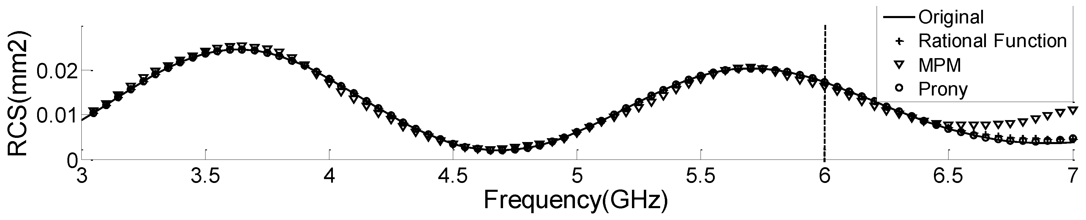
RCS simulation results using CST show that the RCS value gradually converges to a specific level as the frequency increases. The RCS prediction value at 6 GHz to 7 GHz also follows the CST data and tends to converge to a specific level.

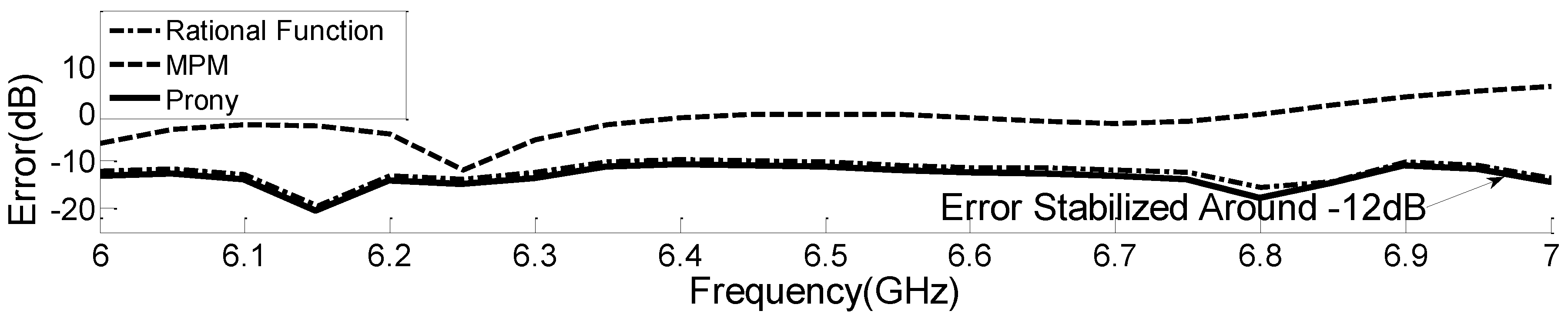
Original data simulated at 21 degrees of the Jet Plane model is compared to values predicted using MPM, Prony and Rational Function in the high-frequency band from 6 GHz to 7 GHz, as shown in Figure 3, the forecast result obtained using the Rational Function method matches the actual data, and its error rise in proportion to frequency increment does not exceed the –10 dB as shown in Figure 4. The Prony method follows the original data better than the Rational Function method’s result, and its error is kept below the average of −12 dB, which is better than the result of the Rational Function method. Meanwhile, compared to the original data, MPM has a larger deviation with increasing frequency, and its inaccuracy climbs to more than −5 dB above 6 GHz and tends to diverge.

In the high-frequency band from 6 GHz to 7 GHz, values from the original data, which was simulated at 18 degrees of the Transport Plane Model, are compared to predictions made using MPM, Prony and Rational Function theories. The forecast result achieved using the Rational Function approach is depicted in Figure 5, which is consistent with the original data. Its error increase as a function of frequency increment does not exceed the –10 dB, as shown in Figure 6. The Prony method data can closely resemble the original one, which is equivalent to or greater than the Rational Function prediction method’s output, and its inaccuracy is similarly within –10 dB. MPM, on the other hand, deviates from the original data as the frequency rises, and its error rises by more than −5 dB over the prior error.

As shown in Figure 7, data predicted using the Rational Function and Prony method at 153 degrees of the F-117 Model follow the original data in the high-frequency band of 6 GHz or more, and its error is kept within the average of –15 dB as shown in Figure 8. The Prony method is more accurate than the Rational Function when it comes to original data. Meanwhile, the data predicted by MPM has a tendency to diverge without tracking the original data, with an inaccuracy of more than −6 dB above the 6 GHz band.

3.2.2. Comparison of Prediction Error Results by Model in All Directions

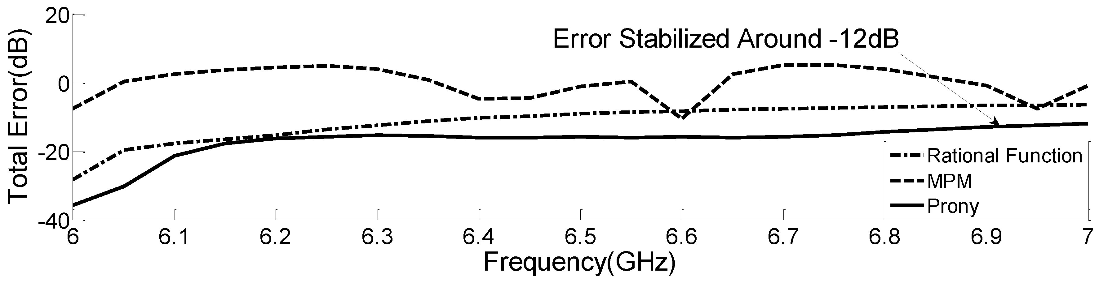
Total errors represent deviation between CST data and prediction results in the 6 GHz–7 GHz. It tends to increase when predicting RCS in the 6 GHz–7 GHz band through prediction theory in all directions, but most of them are stabilized and maintained over a certain part.

The inaccuracy grows as the frequency increases in the Jet Plane model, and its error in all directions is displayed in Figure 9. The error is proportional to frequency growth and is stabilized at −3 dB and −2 dB levels in the Prony method and Rational Function, respectively. However, in the case of MPM, its error tends to increase much more than −2 dB.

The Rational Function maintains the inaccuracy below −7 dB or less when the frequency increases in the Transport Plane model, as shown in Figure 10. In the case of the Prony method, the inaccuracy tends to stay around −12 dB. Regarding the MPM case, there is a propensity for an inaccuracy to fluctuate above −2 dB.

The inaccuracy in the F-114 model grows with frequency, and its error in all directions is indicated in Figure 11. As the frequency increases, the Rational Function maintains the error below −8 dB, whereas the Prony method gradually increases but tends to converge at −12 dB. In the meantime, in the case of MPM, its error tends to exceed –5 dB.

3.2.3. Comparison of Simulation Time Based on Prediction Theories

Three prediction theories were applied to three military aircraft in order to reduce the amount of time needed in the high-frequency band as assessed by CST. The measurement times of aircraft applied with the three prediction theories were then verified in order to confirm whether or not they were much shorter than those obtained from the CST simulation. The measured time was found through the index presented in the simulation software.

In the high-frequency band, the measurement time required an average of 60 h or more for each model using the CST STUDIO software, and the measurement time increased with higher frequencies.

When each prediction theory was applied to each aircraft model,

Table 2. Simulation time comparison among CST and prediction theories.

Method	Frequency (GHz)	Time
		Jet Plane	Transport Plane	F-117
CST	6–7	60 h	80 h	85 h
Rational Function	6–7	1.342 s	1.462 s	1.699 s
MPM	6–7	1.298 s	1.330 s	1.767 s
Prony	6–7	1.363 s	1.348 s	1.688 s

shows the measurement duration of each prediction method per model in the time-consuming 6 GHz to 7 GHz high-frequency band. It required a minimum of 1.342 s and a maximum of 1.699 s for the Rational Function, a minimum of 1.298 s and a maximum of 1.767 s for MPM and a minimum of 1.363 s and a maximum of 1.688 s for the Prony method. It was found that the time measured through prediction theories in the high-frequency band was within a few seconds.

As a consequence, given that the measurement time of the original data in the high-frequency band using CST was taken 60 h or more, the computation time measured using prediction theories was faster than the time measured using CST in the high-frequency range. It was confirmed that the measurement using prediction theory is able to greatly reduce the necessary time. It was also discovered that there was no difference in simulation time between prediction approaches, including the Prony method in the high-frequency range.

3.2.4. Prediction Results in All Directions at 7 GHz

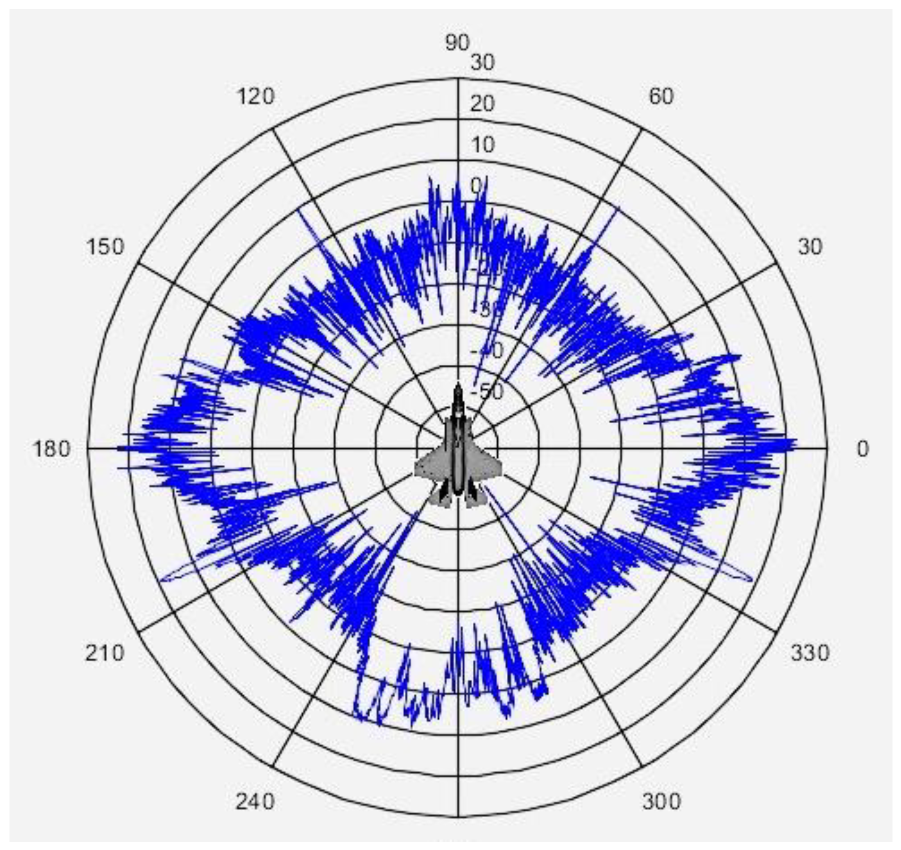
The original RCS data measured in the omnidirectional condition at 7 GHz was compared to the RCS data predicted by each prediction theory under the same conditions.

The findings of the comparison where each prediction theory was applied in the three models indicated that the prediction data to which the MPM was applied in all models hardly follows the original data and that there are many divergences, as shown in Figure 12, Figure 13 and Figure 14. Especially the Jet Plane model in Figure 12 has a deviation throughout the full range compared to the original data, while the Transport Plane model in Figure 13 has divergence at ±140 deg and ±170 deg. At ±30 degrees and ±150 degrees, the deviation in the F-117 model tends to grow compared to the original data in Figure 14.

The Rational Function’s prediction data largely follows the original data; however, there are some deviations Figure 12 shows deviations from the original data at numerous angles, including ±20 degrees and ±100 degrees in the Jet Plane model, and Figure 13 shows deviations at multiple angles, including ±45 degrees and ±115 degrees in the Transport Plane model. Figure 14 also illustrates deviations from the original data at multiple angles, including ±30 degrees and ±150 degrees in the F-117 model.

Meanwhile, the forecast data to which Prony Method is applied has minor deviations at a particular angle, but it generally follows the original data and is the most similar to the original data of the three prediction theories. The Jet Plane model of Figure 12 shows deviations at some angles compared to the original, but it follows the original data well. There are variations at ±50 degrees and ±70 degrees in the Transport Plane model of Figure 13, but overall it looks similar to the original data. Figure 14 shows the F-117 model following the original data from several viewpoints.

4. Conclusions

The indirect calculation method is preferred over the actual measurement method in RCS measurement due to cost and time constraints. However, the method has various drawbacks, including increased analysis time and increasing inaccuracy with frequency increment. To compensate for these flaws, researchers have lately attempted to predict RCS at a high frequency using prediction theories. The Rational Function is one of the prediction theories that have been recently studied for RCS measurement, and it was found that its prediction result has accuracy within the allowed error range in the high-frequency band throughout the study.

In this paper, the RCS data in the high-frequency band is predicted using not only the Rational Function prediction theory introduced in previous papers but also the Prony and MPM prediction theories that have not been used in RCS high-frequency measurement on aircraft models such as Jet Plane, F-117 and Transport Plane in order to find the most efficient RCS measurement method. Through the use of prediction methods on models, comparative research of prediction methods was conducted. In terms of measurement time, all prediction methods have been demonstrated to be significantly faster than the measurement time of the original data obtained in the CST simulation. In addition, as for the accuracy of each prediction method’s outcome, three prediction methods, such as Prony, MPM and Rational Function, are applied to three different types of aircraft models in order to predict RCS at high-frequency band, and the prediction results are compared to one another, confirming that the Prony method closely follows the original data and has the least error among them.

5. Future Works

Several theories were considered when selecting the prediction theory to be applied for this study, but in the end, the theories with somewhat effective prediction results were compressed into three.

Based on this prediction theory, it is founded that the Prony method has a good result in RCS prediction at high-frequency under restricted conditions, such as three prediction methods and three military aircraft models in this paper. However, in order to generalize that the method is optimal, it is required to conduct an expanded study in addition to the three prediction methods and aircraft models applied in this paper.

References

- Hu, C.; Li, N.; Chen, W.; Guo, S. Improving Precision of RCS Measurement Based on Spectral Extrapolation Method. In Proceedings of the 2020 International Applied Computational Electromagnetics Society Symposium, Monterey, CA, USA, 27–31 July 2020. [Google Scholar]
- Touzopoulos, P.; Boviatsis, D.; Zikidis, K. Constructing a 3D model of a complex object from 2D images for the purpose of estimating its Radar Cross Section (RCS). J. Comput. Modeing 2017, 7, 15–28. [Google Scholar]
- Rezende, M.C.; Martin, I.M.; Faez, R.; Souza Miacci, M.A.; Nohara, E.L. Radar Cross Section Measurements (8–12 GHz) of Magnetic and Dielectric Microwave Absorbing Thin Sheets. Rev. Fısica Apl. Instrum. 2002, 15, 24–29. [Google Scholar]
- Öztürk, A.K. Implementation of Physical Theory of Diffraction for Radar Cross Section Calculations. Master’s Thesis, Bilkent University, Ankara, Turkey, July 2002. [Google Scholar]
- Weinmann, F. Ray tracing with PO/PTD for RCS modeling of large complex objects. IEEE Trans. Antennas Propag. 2006, 54, 1797–1806. [Google Scholar] [CrossRef]
- Harrington, R.F. Field Computation by Moment Methods; Macmillan: New York, NY, USA, 1968. [Google Scholar]
- Peterson, A.; Mittra, R. Iterative-based computational methods for electromagnetic scattering from individual or periodic structures. IEEE J. Ocean. Eng. 1987, 12, 458–465. [Google Scholar] [CrossRef]
- Mihai, I.V.; Tamas, R.; Sharaiha, A. An UWB Physical Optics Approach for Fresnel-Zone RCS Measurements on a Complex Target at Non-Normal Incidence. Sensors 2019, 19, 5454. [Google Scholar] [CrossRef] [Green Version]
- Yamada, Y.; Michishita, N.; Nguyen, Q.D. Calculation and measurement methods for RCS of a scale model airplane. In Proceedings of the 2014 International Conference on Advanced Technologies for Communications, Hanoi, Vietnam, 15–17 October 2014. [Google Scholar]
- Hu, C.; Li, N.; Chen, W.; Zhang, L. High-precision RCS measurement of aircraft’s weak scattering source. Chin. J. Aeronaut. 2016, 29, 772–778. [Google Scholar] [CrossRef] [Green Version]
- Kim, W.; Lm, H.; Noh, Y.; Hong, I.; Tae, H.; Kim, J.; Yook, J. Near-Field to Far-Field RCS Prediction on Arbitrary Scanning Surfaces Based on Spherical Wave Expansion. Sensors 2020, 20, 7199. [Google Scholar] [CrossRef]
- Liu, Y.; Hu, W.; Zhang, W.; Sun, J.; Xing, B.; Ligthart, L. Radar Cross Section Near-Field to Far-Field Prediction for Isotropic-point Scattering Target Based on Regression Estimation. Sensors 2020, 20, 6023. [Google Scholar] [CrossRef]
- Kong, W.; Zheng, Y.; Song, Y.; Fang, Z.; Yang, X.; Zhang, H. Analysis of Wideband Scattering from Antenna Based on RFGG-FG-FFT with Cube Polynomial Inter/Extrapolation Method. Appl. Sci. 2022, 12, 10298. [Google Scholar] [CrossRef]
- Pablo, S.; Lorena, L.; Alvaro, S.; Felipe, C. EM Modelling of Monostatic RCS for Different Complex Targets in the Near-Field Range: Experimental Evaluation for Traffic Applications. Electronics 2020, 9, 1890. [Google Scholar]
- Zhao, H.; Shen, Z. Fast Wideband Analysis of Reverberation Chambers Using Hybrid Discrete Singular Convolution-Method of Moments and Adaptive Frequency Sampling. IEEE Trans. Magn. 2015, 51, 1–4. [Google Scholar] [CrossRef]
- Seol, K.; Koh, J.; Han, S. RCS Prediction using Cauchy method with Increasing Prediction Frequency. In Proceedings of the 2018 IEEE International Conference on Consumer Electronics, Las Vegas, NV, USA, 12–14 January 2018. [Google Scholar]
- Seol, K.; Cho, W.; Kang, G.; Koh, J. RCS at High Frequency Band using Rational Functions. In Proceedings of the 2018 IEEE International Symposium on Antennas and Propagation & USNC/URSI National Radio Science Meeting, Boston, MA, USA, 8–13 July 2018. [Google Scholar]
- Koh, J. High-Frequency RCS Estimation. In Proceedings of the 2019 IEEE International Conference on Aerospace Electronics and Remote Sensing Technology, Yogyakarta, Indonesia, 17–18 October 2019. [Google Scholar]
- Andres, G.; Francisco, R.; Edwin, P. Vector Fitting–Cauchy Method for the Extraction of Complex Natural Resonances in Ground Penetrating Radar Operations. Algorithms 2022, 15, 235. [Google Scholar]
- Nattawat, C.; Boonpoonga, A. Radar target identification of coated object using cauchy method. In Proceedings of the 2015 IEEE International Conference on Antenna Measurements & Applications, Chiang Mai, Thailand, 30 November–2 December 2015. [Google Scholar]
- Singh, S. Application of Prony Analysis to Characterize Pulsed Corona Reactor Measurements. Master’s Thesis, University of Wyoming, Laramie, WY, USA, January 2003. [Google Scholar]
- Hildebrand, F.B. Introduction to Numerical Analysis, 2nd ed.; McGraw-Hill Press: New York, NY, USA, 1987. [Google Scholar]
- Ko, W.L.; Mittra, R. A combination of FD-TD and Prony's methods for analyzing microwave integrated circuits. IEEE Trans. Microw. Theory Tech. 1991, 39, 2176–2181. [Google Scholar] [CrossRef]
- Khodadadi Arpanahi, M.; Kordi, M.; Torkzadeh, R.; Haes Alhelou, H.; Siano, P. An Augmented Prony Method for Power System Oscillation Analysis Using Synchrophasor Data. Engines 2019, 12, 1267. [Google Scholar] [CrossRef]
- Sarrazin, F.; Sharaiha, A.; Pouliguen, P.; Chauveau, J.; Collardey, S.; Potier, P. Comparision between Matirx Pencil and Prony methods applied on nosiy antenna responses. In Proceedings of the 2011 Loughborough Antennas & Propagation Conference, Loughborough, UK, 14–15 November 2011. [Google Scholar]
- Hussen, A.; He, W. Prony Method for Two-Generator Sparse Expansion Problem. Math. Comput. Appl. 2022, 27, 60. [Google Scholar]
- Luis, A.T.G.; Miguel, A.P.G.; Johnny, R.M.; Mario, A.G.V.; Luis, H.R.A.; Fernando, S.S. Prony Method Estimation for Motor Current Signal Analysis Diagnostics in Rotor Cage Induction Motors. Energies. 2022, 15, 3513. [Google Scholar]
- Zhang, S.; Liu, G.; Li, Y.; Yao, J. Householder-based Prony Method for Identification of Low-frequency Oscillation in Power System. In Proceedings of the 2019 4th International Conference on Advances in Energy and Environment Research, Hefei, China, 1–3 November 2019. [Google Scholar]
- Kheawprae, F.; Boonpoonga, A.; Sangchai, W. Measurement for radar target identification using short-time matrix pencil method. In Proceedings of the 2015 IEEE Conference on Antenna Measurements & Applications, Chiang Mai, Thailand, 30 November–2 December 2015. [Google Scholar]
- Hua, Y.; Sarkar, T.K. Matrix pencil and System poles. Signal Process. 1990, 21, 195–198. [Google Scholar] [CrossRef] [Green Version]
- Hua, Y.; Sarkar, T.K. Matrix pencil methods for estimating parameters of exponentially damped/undamped sinusoids in noise. IEEE Trans. Acoust. Speech Signal Process. 1990, 38, 814–824. [Google Scholar] [CrossRef] [Green Version]
- Rousafi, A.; Fortino, N.; Dauvignac, J.Y. UWB antenna 3D characterization using Matrix Pencil method. In Proceedings of the 2014 IEEE Conference on Antenna Measurements & Applications, Antibes, France, 16–19 November 2014. [Google Scholar]
- Reginelli, N.F.; Sakar, T.K.; Salazar-Palma, M. Interpolation of Missing Antenna Measurements or RCS Data Using the Matrix Pencil Method. In Proceedings of the 2018 15th European Radar Conference, Madrid, Spain, 26–28 September 2018. [Google Scholar]
- Chamaani, S.; Akbarpour, A.; Helbig, M.; Sachs, J. Matrix Pencil Method for Vital Sign Detection from Signals Acquired by Microwave Sensors. Sensors 2021, 21, 5735. [Google Scholar] [CrossRef]
- Chaparro-Arce, D.; Gutierrez, S.; Gallego, A.; Pedraza, C.; Vega, F.; Gutierrez, C. Locating Ships Using Time Reversal and Matrix Pencil Method by Their Underwater Acoustic Signals. Sensors 2021, 21, 5065. [Google Scholar] [CrossRef]
- Shao, X.; Hu, T.; Zhang, J.; Li, L.; Xiao, M.; Xiao, Z. Efficient Beampattern Synthesis for Sparse Frequency Diverse Array via Matrix Pencil Method. Sensors 2022, 22, 1042. [Google Scholar] [CrossRef] [PubMed]
- Department of Defense. MIL-HDBK-1797 Department of Defense Handbook Flying Qualities of Piloted Aircraft; Department of Defense: Washington, DC, USA, 1997.