Article

Range-Based Reactive Deployment of a Flying Robot for Target Coverage

1
Department of Aeronautical and Aviation Engineering, The Hong Kong Polytechnic University, Hong Kong 999077, China
2
Department of Automation, Harbin Institute of Technology, Shenzhen 518055, China
3
Research Centre for Unmanned Autonomous Systems, The Hong Kong Polytechnic University, Hong Kong 999077, China
*
Author to whom correspondence should be addressed.
Aerospace 2022, 9(11), 731; https://doi.org/10.3390/aerospace9110731
Submission received: 12 October 2022 / Revised: 13 November 2022 / Accepted: 18 November 2022 / Published: 20 November 2022
(This article belongs to the Special Issue Energy Efficiency of Small-Scale UAVs)

Abstract

:
Flying robots, also known as drones and unmanned aerial vehicles (UAVs), have found numerous applications in civilian domains thanks to their excellent mobility and reduced cost. In this paper, we focus on a scenario of a flying robot monitoring a set of targets, which are assumed to be moving as a group, to which the sparse distribution of the targets is not applicable. In particular, the problem of finding the optimal position for the flying robot such that all the targets can be monitored by the on-board ground facing camera is considered. The studied problem can be formulated as the conventional smallest circle problem if all the targets’ locations are given. Because it may be difficult to obtain the locations in practice, such as in Global Navigation Satellite Systems (GNSS) dined environments, a range-based navigation algorithm based on the sliding mode control method is proposed. This algorithm navigates the flying robot toward the farthest target dynamically, using the estimated robot–target distances from the received signal strength, until the maximum robot–target distance cannot be further reduced. It is light computation and easily implementable, and both features help to improve the energy efficiency of the flying robot because no heavy computation is required and no special sensing device needs to be installed on the flying robot. The presented solution does not directly solve the smallest circle problem. Instead, our proposed method dynamically navigates the flying robot to the center of the group of targets using the extracted distance information only. Simulations in Matlab and Gazebo have been conducted for both stationery and mobile targets to verify the effectiveness of the proposed approach.

1. Introduction

Thanks to the decreasing cost and advanced control methods [1,2] developed in recent years, flying robots have been widely applied in various applications including, but not limited to, inspections [3], target tracking [4,5], monitoring and surveillance [6,7], wireless communication support [8], data collection or dissemination from or to wireless sensor networks (WSNs) [9], etc. Among these applications, a particularly prominent issue is the deployment of flying robots. With proper deployment, the flying robots can bring much more benefits than the conventional static servicing system, especially when mobility is involved, such as the mobile targets in the surveillance scenario, the mobile users in the case of wireless communication support, and the mobile sensors in WSNs.
This paper considers the application of using a flying robot to monitor a set of targets and/or support their communication with a remote ground base station. A typical example is shown in Figure 1. A group of hikers walks in the mountains. A remote base station wishes to acquire the real-time status of the hikers for safety purposes. Consider the scenario in which the team goes into an area where the communication with the remote base station is blocked by some environmental obstacles such as mountains. In such a case, a flying robot can fly to the hikers to monitor them with the onboard camera and serve as a relay for communication between the remote base station and the hikers. There are several requirements for the flying robot. First, it needs to keep all the hikers within vision. Second, it needs to operate in an energy-efficient way to prolong its service time, due to the limited onboard battery capacity. Finally, it needs to remain within the communication range of the remote base station to maintain the valid backhaul link.
Under such a scenario, the focus is on navigating the flying robot from an initial position to a destination where the first two aforementioned requirements are met. In practice, the flying robot also needs to stay within the communication range of the remote base station. Since this issue can be addressed by introducing some relays between the flying robot and the remote base station, this paper assumes that the flying robot has a valid backhaul link with the remote base station.
There are two critical issues in the problem of interest. The first one is the determination of the destination and the second one is how to navigate the flying robot toward such a destination. To achieve these objectives, the following aspects are considered. Considering that the lower altitude generally leads to a better surveillance performance, the aim of the deployment of the flying robot is to find the relatively low altitude while ensuring the surveillance of all the targets. Consider that the flying robot is equipped with a camera with a fixed angle of vision. Thus, the coverage area can be regarded as a disk and the radius is proportional to the altitude [10]. With the energy consumption model and the coverage area model, one can figure out some characteristics of the destination: the 2D projection of the destination should be the center of the smallest circle that encloses all the targets and its altitude should ensure the coverage of the smallest circle radius.
Clearly, this is the conventional smallest circle problem [11]. Given the locations of targets, the optimal projection can be found, and then the altitude can be computed following the coverage area model. However, in practice, the locations of targets may not be obtained easily, especially when the targets are mobile. Thus, the destination may not be computed in advance.
For the problem considered, a range-based reactive algorithm is proposed to navigate the flying robot to the center of the smallest circle enclosing all the targets. This algorithm does not require knowing the targets’ locations in advance. It is assumed that the flying robot, launching from the initial position, can fly to a position where it can get Line-of-Sight (LoS) communication links with the targets. The last track of targets’ locations at the remote base station can be used. Additionally, when the targets lose communications with the remote base station, they periodically broadcast a beacon message, which can be received by the flying robot if it is around. From the received signal strength indicator (RSSI), the flying robot estimates the corresponding distances from the targets to itself. From the estimated robot-target distances, the robot uses the largest one for navigation. Then, it always flies towards the farthest target, until the maximum robot–target distance cannot be further reduced. To facilitate the recognition of reaching the smallest circle center, two conditions derived from the features of the smallest circle are presented; and to support checking these two conditions, the robot needs to estimate a few targets’ locations based on the robot–target distances. As shown later, for an arbitrary distribution of targets, the robot needs to estimate 5 targets’ locations.
To evaluate the effectiveness of the proposed algorithm, extensive computer simulations have been conducted and comparisons with the optimal solutions by Welzl’s algorithm [11] are presented.
A major advantage of the proposed method lies in the light computational complexity and simple RSSI measurement. Both features are significant to a small-size flying robot. Firstly, the algorithm with light computational complexity does not require expensive computing hardware to be installed on the robot, and it can be easily implemented in real time. The RSSI measurement can be obtained from a normal transceiver, which does not require special sensing devices. These features can reduce the payload of the flying robot, which facilitates flying energy efficiency since a larger payload induces higher power consumption. This paper adopts some existing methods and combines them to solve the problem of concern. Although the relevant techniques have been existing, the main contribution is the presented solution that combines these techniques to navigate a flying robot toward a group of moving targets whose locations are unknown. The considered problem can indeed be formulated as the smallest circle problem. However, existing solutions require the location information of each target. However, in the considered problem, location information may not always be available such as in Global Navigation Satellite Systems (GNSS) denied environments. So, the proposed solution does not explore using location information. Instead, we make use of the signal strength to extract range information. We do not target providing another method to solve it. Our proposed method dynamically navigates the flying robot to the center of the group of targets using the extracted range information.
The rest of the paper is organized as follows. Section 2 discusses some relevant works in literature. Section 3 presents the system models and formally states the studied problem. Section 4 presents the details of the proposed range-based reactive navigation algorithm. Section 5 presents the simulation results to demonstrate the performance of the proposed method. Finally, Section 6 concludes the paper and points out a future research direction.

2. Related Work

The deployment of flying robots has received much attention in recent years, due to their flexibility and mobility, and the potential application domains. In the literature, there are two approaches to the problem of deploying flying robots: proactive deployment and reactive deployment.
Proactive deployment usually considers the static scenario, where the necessary resources are available in advance. In particular, there has been extensive work on proactive deployment, with many mature approaches proposed in the design [12,13], control [14,15], and local planning [16] for flying robots. Some existing publications focus on the deployment of a single-flying robot. In [17], the authors propose a closed form of air-to-ground wireless communication channel model that accounts for both LoS link and Non-LoS link. Based on this model, the authors find the optimal altitude for the flying robot such that the coverage area is maximized. Following this model, the paper [18] aims at optimizing both the altitude and the horizontal position. The authors propose an energy-efficient scheme to maximize the number of covered targets, which first sets the vertical position at the altitude providing the maximal coverage, and then optimizes the horizontal position to maximize the covered number using minimum transmitting power.
Rather than decoupling the problem, the paper [19] formulates a mixed integer non-linear problem to select the optimal position from a given set of candidates. In [20], the authors further consider the backhaul connectivity directly to the nearby terrestrial base station on the base of wireless coverage to all ground targets. The paper [21] also studies the power efficiency of a drone base station providing wireless coverage for ground users and formalizes a drone base station placement problem that minimizes the average transmit power of the drone base station. A successive convex approximation-based drone base station placement algorithm is proposed to obtain the optimal drone base station location. In [19], the authors formulate the drone cell placement problem as a 3D placement problem to maximize the revenue of the network. The paper formulates an equivalent quadratically-constrained mixed integer non-linear optimization problem and proposes a computationally efficient numerical solution for this problem. The paper [22] addresses several challenges including coverage of a larger geographical area and data communication links for smart city remote traffic monitoring. The author proposed a reliable drone-based monitoring scheme for a smart city transportation system using an enhanced Ant Colony Optimization technique.
There are also some publications focusing on the deployment of multiple flying robots. In [23], given the locations of targets, the authors propose a K-means clustering-based algorithm to compute the positions of flying robots, to offload the demand for the stationary base stations. Based on the target distribution over a geographical area, the reference [24] proposes a neural-based cost function approach to assign flying robots based on demand. A similar concept, i.e., target density, has also been used [8,25]. The paper [8] proposes a decentralized algorithm to minimize the average robot–target distance by moving the robots toward the centers of mass from some initial positions. The paper [25] considers maximizing the coverage of targets accounting for the charging requirement of flying robots.
The paper [26] proposes a two-phase evolution optimal 3D drone layout algorithm to deploy drones in pipeline networks. A 3D pipeline graph model is designed to represent the possible projection position of drones, and the objective function is proposed for optimal drone deployment. In [27], the authors propose an optimization model that maximizes the coverage of users while minimizing the communication cost between drones. The paper [28] proposes the novel DroneCells scenario where drones constantly move within the cell to serve the users from a closer distance and thus improve the spectral efficiency of the network and the quality of service of cell-edge users. The authors propose practically feasible drone mobility control algorithms with varying complexity and performance.
Although different schemes consider different objectives, one similarity of the aforementioned publications is to optimize the positions for a certain number of flying robots. Another group of references under the category of proactive deployment focuses on minimizing the number of flying robots to cover a given set of targets. The authors of [29] formulate a 2D Geometric Disk Cover problem and propose a centralized heuristic algorithm. Beyond this, the authors of [30] consider the 3D case with the same objective and propose a PSO-based heuristic algorithm. The paper [31] studies a similar problem and presents an elitist non-dominated sorting genetic algorithm to find the optimal positions from a given set of candidates. The reference [6] formulates a mixed integer non-linear optimization model and presents a mixed integer programming-based heuristic algorithm to continuously cover a set of targets. The paper [32] considers a similar problem with [6], and the authors propose a localized heuristic algorithm. Moreover, the publication [33] examines the case with multiple subareas accounting for the charging requirement of flying robots. The authors partition the coverage graph into cycles and the number of flying robots required depends on the charging time, the traveling time, and the number of subareas to be covered by the cycle. The reference [34] also considers the connectivity requirement as [8]. The authors propose a method to decouple the minimum robot number problem into a master program and a pricing program, where the former ensures complete coverage of targets all the time depending on their current locations, and the latter figures out a subset of connected positions from a set of candidates. In [35], every point of very uneven terrain is aimed to be covered with drones, and this problem may be viewed as a drone version of the 3D Art Gallery Problem. A computationally simple algorithm was developed to give an upper estimate of the minimal number of drones necessary and calculate their locations for coverage.
The second approach is for reactive deployment, which aims at designing online algorithms. Assuming that the flying robot can measure the targets’ coordinates, the flying robot can compute and track the center of mass [36]. In [37], the authors introduced an online method to generate a trajectory that facilitates the perception task, which relies solely on onboard, visual-inertial sensors and computing. In their experiments, full state estimation is provided by fusing detections from an onboard camera and an IMU. With the same assumption, the authors of [38] propose a game theory-based navigation algorithm to boost network capacity. The exhaustive search is used to find a potential moving direction at each flying robot. These two schemes are both based on knowing the coordinates of all the targets all the time. Measuring coordinates in practice is difficult or at least costly if some specific protocols and/or sensors are used. When drones fly outdoors, we need to consider their adaptability to changes on the fly, in [39] they tackle the problem of flying a quadrotor using time-optimal control policies that can be replanned online when the environment changes or when encountering unknown disturbances. Another reactive approach is based on virtual forces [40]. The authors propose a reactive algorithm based on four types of virtual forces: hotspots attractive force, user attractive force, nearby robot repulsive force, and obstacle repulsive force. One shortcoming of this method is the assumption that hotspots’ locations should always be known before the deployment of flying robots.
In [41], an online path planning method for a single UAV to periodically cover a set of moving targets on flat ground or uneven terrain is put forward, which is further extended to navigate multiple UAVs for the sensing coverage of moving targets based on the shared information about targets among UAVs. The paper [36] introduces a framework for self-organizing flying radio access networks with ultra-low altitude flying base stations that are automatically positioned in real time according to the users’ requirements and mobility. The proposed concept enables optimization of the network in real-time according to the users’ throughput requirements and movement, enabling massive exploitation of higher frequency bands for communication and higher energy efficiency.
The authors of [6] formulate the mobile targets covering the problem using drones and mathematically define mixed integer non-linear optimization models. The aim is to locate UAVs to cover the piece of the plane in which the target moves by using a minimum number of UAVs. In [40], the paper proposes the problem of how to deploy multiple UAVs for on-demand coverage while at the same time maintaining the connectivity among UAVs. The authors propose two algorithms: a centralized deployment algorithm and a distributed motion control algorithm, which, respectively, require a minimum number of UAVs to provide desirable service and enable each UAV to autonomously control its motion, find the user equipment and converge to on-demand coverage without global information.
The paper [42] formulates the deploying flying robot base stations problem to bridge the affected users to a cellular network based on the scenario where the stationary base stations in some disaster areas are destroyed. The authors propose an optimization model to maximize the quality of coverage with local information and require the flying robot to always keep a safe distance to avoid collision while moving. The approach presented in the current paper falls into this category. Different from the existing publications, the information on coordinates is not assumed to be known in the proposed approach.

3. Problem Statement

This section formally states the studied problem. The main symbols used in this paper are summarized in Table 1 for quick reference.
Consider a set of m ( m > 1 ) targets on a 2D plane. Let s j or ( s j x , s j y ) denote the 2D location of target j ( j = 1 , , m ), which is not known in advance. We first consider that the targets are static and the mobile case will be discussed in the next section. Considering the example of Figure 1, this scenario of static targets can be that after losing good quality communication with the remote base station, the targets stop moving and wait for the flying robot. A flying robot can move in 3D space, but the altitude is constrained by the range [ Z m i n , Z m a x ] . At any time t, the position of the flying robot is represented by P ( t ) = ( x ( t ) , y ( t ) , z ( t ) ) and θ ( t ) is the horizontal heading. We consider the following motion model for the flying robot [43]:
x ˙ ( t ) = v ( t ) cos ( θ ( t ) ) , y ˙ ( t ) = v ( t ) sin ( θ ( t ) ) , θ ˙ ( t ) = u ( t ) , z ˙ ( t ) = w ( t ) .
where v ( t ) { 0 , v ¯ } is the horizontal speed, u ( t ) [ u ¯ , u ¯ ] is the angular velocity, and  w ( t ) [ w ¯ , w ¯ ] is the vertical speed. For simplicity, we consider the movement of the flying robot in horizontal and vertical directions separately. When it moves horizontally, w ( t ) = 0 ; while, when it moves vertically, u ( t ) = 0 and v ( t ) = 0 .
The robot carries a ground-facing camera to monitor the targets. The camera is with a fixed visibility angle φ . The coverage area by the robot at time t is a disk centered at ( x ( t ) , y ( t ) ) with the radius [10], see Figure 1:
r ( t ) = z ( t ) tan φ 2 .
With the coverage model, the considered problem can be formulated as follows:
min x ( t ) , y ( t ) , z ( t ) z ( t )
s . t . ( x ( t ) s j x ( t ) ) 2 + ( y ( t ) s j y ( t ) ) 2 1 2 z ( t ) tan φ 2 , j .
Obviously, problem (3) is the conventional smallest circle problem [11], which can be solved by a simple randomized algorithm if all the locations of targets are known. However, in the considered context, the targets’ locations are not known in advance. One naive idea to obtain the targets’ locations is via the onboard camera. If the flying robot can fly high enough to view all the sensors, it can then obtain the locations of targets through image processing. With all the targets’ locations, the smallest circle problem can be addressed, and the optimal position of the flying robot can also be found. However, this method may not be realistic, since in practice the allowed deployment altitude is constrained by regulation. When the flying robot starts from the remote base station in Figure 1, even when it flies to Z m a x , it cannot see all the targets; see Figure 2. In the next section, we propose our RSSI-based method to solve this problem.

4. Proposed Solution

This section presents an algorithm to reactively navigate the flying robot toward the center of the smallest circle. The proposed algorithm does not require the targets’ locations in advance. Instead, it requires the robot to estimate the range between the flying robot and a target from the received signal strength [44]. Thus, the proposed method is a range-based navigation method. Although the exact targets’ locations are unknown, the system may know the rough location of the targets. In the example mentioned in the introduction, before the targets go into an area with poor communication channels, the remote base station can know their last location. Thus, the flying robot can first fly to such a position. At this position, it is assumed that the flying robot can have LoS communication links with targets. Measured in decibels at the flying robot, the RSSI from target j, i.e.,  p j ( t ) , can be modeled as follows [45]:
p j ( t ) = p t 10 ε log D j ( t ) + ν j ( t ) ,
where p t is a constant depending on the transmitted power, wavelength, as well as antenna gain of the flying robot, ε is a slope index depending on the environment, ν j ( t ) is the logarithm of the shadowing component, and  D j ( t ) is the 3D Euclidean distance between the flying robot and target j. In this paper, fast fading is not considered by assuming a low-pass filter is used to attenuate Rayleigh or Rician fade.
The robot–target distance D j ( t ) can be further expressed in terms of the target’s coordinates, i.e.,  ( s j x , s j y ) :
D j ( t ) = ( x ( t ) s j x ) 2 + ( y ( t ) s j y ) 2 + z 2 ( t ) 1 2
Let d j ( t ) denote the 2D distance between the robot projection and target j. The 2D projection-target distance d j ( t ) can be easily computed from the 3D robot–target distance D j ( t ) , since the altitude of the flying robot z ( t ) is known to itself. Further, let d ˙ j ( t ) denote the derivative of the 2D projection–target distance d j ( t ) , which can also be known to the robot. Moreover, the flying robot can also estimate the targets’ locations from either projection–target or robot–target distances by existing algorithms, such as the extended Kalman filter. Notice that such locations are not used for navigation; instead, they are used to judge whether the flying robot reaches the smallest circle center.
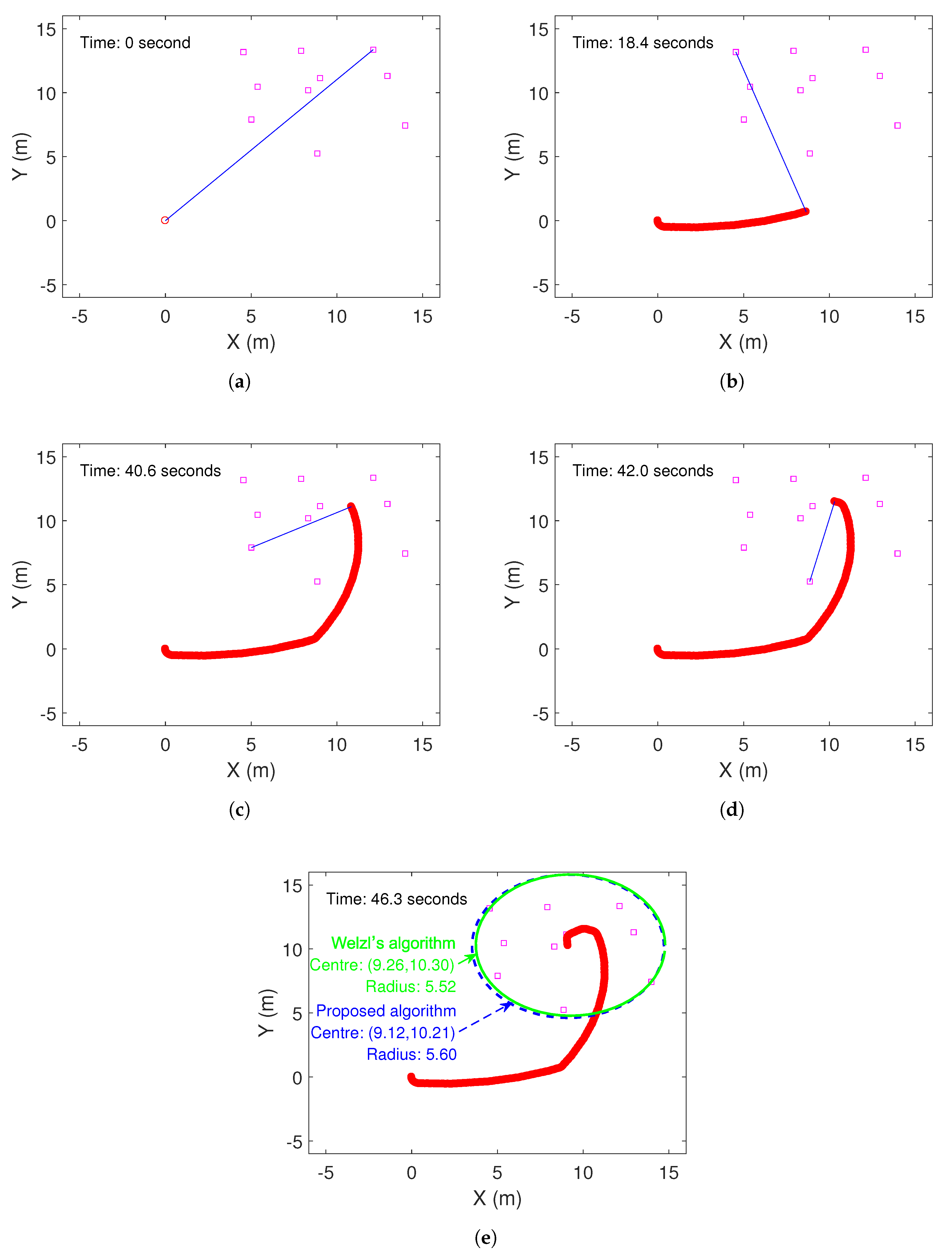
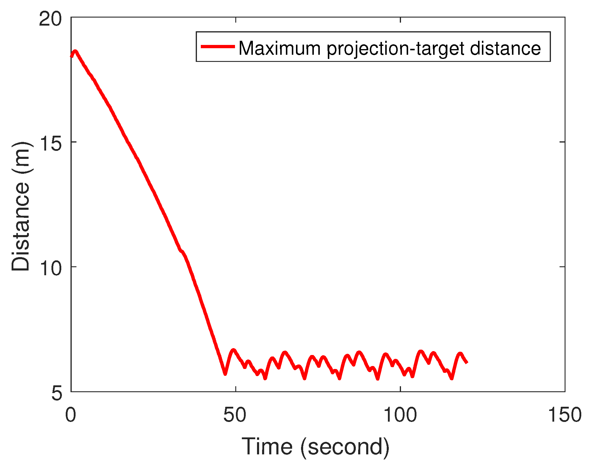
Now, it is the position to present the proposed navigation algorithm. The basic idea is to reduce the largest projection–target distance recursively, and when the maximum projection–target distance cannot be further reduced, the flying robot reaches the smallest circle center. Two keys of this algorithm are how to navigate the robot toward the farthest target and how to judge whether the maximum projection–target distance cannot be further reduced.
For the first component, the following navigation law can be adopted:
u ( t ) = sgn { d ˙ ( t ) + Λ [ d ( t ) d 0 ] } u ¯ ,
where
sgn ( α ) = 1 , if α > 0 , 0 , if α = 0 , 1 , if α < 0 ,
Λ ( β ) = γ β , if | β | δ , sgn ( β ) γ δ , otherwise .
Here, γ and δ are some given positive parameters. This navigation law has been successfully used in obstacle avoidance [46] and environmental level sets tracking [47]. Here, we need to examine if this navigation law can be adopted for the said purpose. In [46], d 0 is the minimum distance from obstacles; while in [47], d 0 is the pre-specified environmental parameter and the goal is to navigate a ground robot to track such level. In this paper, d 0 is the distance at which the robot is regarded as reaching a target. Since the objective is not to reach a specific target, d 0 can be simply set as a small value. By doing so, the flying robot will not stop before it comes to the proximity of the targets.
Deciding whether the maximum projection–target distance can be further reduced is difficult for an online algorithm, since the flying robot may not know the projection–target distances for the future. To this end, it is necessary to find an alternative way to assist the flying robot to check whether the optimal position has been reached. Below, two conditions based on the features of the smallest circle are presented.
Specifically, there should exist at least two targets on the smallest circle and all the other targets are inside the circle. For the case with two targets on the circle, say s 1 and s 2 , the straight line linking these two targets is the diameter of the smallest circle. Thus, one can have:
d 1 = d 2 = 1 2 s 1 s 2 , d j < d 1 , j = 3 , , m ,
where s 1 and s 2 are also used to represent the estimated locations of targets s 1 and s 2 , respectively, d 1 and d 2 are the projection-distance distances, respectively, and  s 1 s 2 is the 2D distance between targets s 1 and s 2 .
For the case with more than two targets on the circle, say s 1 , , s k , k 3 , one can have the following features:
d 1 = d 2 = = d k > d j , j = k + 1 , , m , Δ s j a s j b s j c is a non-obtuse triangle , j a , j b , j c [ 1 , k ] .
Δ s j a s j b s j c represents the triangle formed by the targets s j a , s j b and s j c . It requires that there exists at least one set of three targets forming an acute triangle or a right triangle, rather than an obtuse triangle, otherwise the robot is not at the smallest circle center. For example, in Figure 3, the green dotted circle is centered at P 1 , with  s 1 , s 2 and s 3 on the circle and all the others are inside the circle. This is not the smallest circle. Since the triangle formed by s 1 , s 2 and s 3 is an obtuse one, the flying robot can reduce the radius by slightly moving the center towards the target corresponding to the obtuse angle, i.e.,  s 1 . s 1 will still be inside the new circle as well as all the others. The smallest circle for this case is the red dash one, where s 2 , s 3 and s 4 are on the circle and they form an acute triangle.
To verify conditions (7) and (8), the flying robot needs to estimate k targets’ locations, which correspond to the largest k projection–target distances. A statistical method is used to determine k. Simulations with different numbers of targets have been conducted to see how many targets are on the smallest circle. The Welzl’s algorithm [11] is used to determine the smallest circle, and the average results are shown in Figure 4, where many targets (10 to 90) are randomly deployed 1000 times independently. From this result, one can see that the probability of two or three targets on the smallest circle is about 0.9; that of no greater than four targets on the circle is about 0.95, and that of over five targets on the circle is almost 0. Therefore, to implement the proposed algorithm on a flying robot in real time for an arbitrary distribution of targets, k takes 5. Notice that this k value may not be suitable for scenarios with some specific formations; for example, all the targets remain in a circular formation. To make the proposed algorithm work for these cases, the robot will need to estimate all the targets’ locations all the time, which significantly increases the computation load.
The overall algorithm is summarized in Algorithm 1. Here, d i s is the vector of projection-target distances and d i s ˙ is the vector of the derivatives. If the robot has not reached the smallest circle center, it moves closer to the farthest target (Line 5), i.e., reducing the maximum projection-target distance. The flying robot will dynamically change the expected target once another target becomes the farthest one. After reaching the smallest circle center, the robot stops moving horizontally and then moves vertically to the altitude corresponding to the smallest radius (Line 3). It is worth mentioning that in the implementation when the robot checks the first sub-condition of (7) or (8), a threshold is used, i.e., if the gap between the two distances is smaller than the given threshold, (7) or (8) is regarded as satisfied. Notice that Algorithm 1 navigates the flying robot to a position whose projection is the smallest circle center. To have all the targets in vision, the flying robot will further adjust its altitude such that the coverage radius equals that of the smallest circle. If at the highest altitude the camera still cannot cover the smallest circle due to the sparse distribution of the targets, the targets cannot be fully covered. An alternative is to explore the cruising mode, i.e., navigating the flying robot to follow an orbit, which enables the observation of multi-target for a satisfying time interval in a sparse distribution.
Algorithm 1: The range-based reactive navigation algorithm.
Require: d i s and d i s ˙ .
Ensure:u and v.
 1:
Sort d i s and d i s ˙ in decent order according to the distance and for the first k distances, estimate the corresponding targets’ locations.
 2:
if Condition (7) or (8) holds then
 3:
     u = 0 , v = 0 . Compute the altitude using (2) with r replaced by d 1 .
 4:
else
 5:
    Compute control input u according to (6) with d ( t ) and d ˙ ( t ) replaced by d 1 and d ˙ 1 . v = v ¯ .
 6:
end if
The presented method can be extended to the case of mobile targets. Here, we only consider horizontal movement. In this case, the flying robot keeps following the targets instead of stopping to hover. Thus, the tasks of checking conditions (7) or (8) are not necessary, which results in there being no need to estimate the targets’ positions. The flying robot only needs to find out the farthest target and then uses Formula (6) to compute the control input.

5. Simulation Results

This section evaluates the performance of the proposed algorithm via simulations in Matlab and Gazebo. In the simulations presented below, the vertical dimension movement is not considered. The parameters used here are summarized in Table 2.

5.1. Simulations in Matlab

An example with 10 targets randomly deployed in an area with the size of 10 m by 10 m is displayed, see Figure 5a. The initial position and heading of the robot are ( 0 , 0 ) and 3 2 π , which is facing the negative Y axis. The sampling interval is 0.1 s. For checking condition (7) or (8), the distance threshold is set as 0.2 m. It is assumed that the projection–target distances are accurate now and the influence of the noise level will be discussed later. Starting from the initial position, the robot tries to move towards the target in the top-right corner, which is the farthest one. After 18.4 s, the robot changes the expected target to the one on the top-left, see Figure 5b. At 40.6 and 42.0 s, the robot changes target again, see Figure 5c,d. Finally, it reaches the smallest circle center, see Figure 5e. Here, the smallest circle obtained by the proposed approach is presented and compared with Welzl’s algorithm. The outputs of the two algorithms are very close. In Figure 6, the maximum projection–target distance along the path is plotted.
In the beginning, since the robot is heading the negative Y axis and it is constrained by the maximum angular velocity u ¯ , it tries to rotate, which makes the maximum projection–target distance increase a little. After that, such distance keeps decreasing until reaching the smallest circle center. Further, more simulation results for a different number of targets are presented. The results are summarized in Table 3. From this table, one can see that the proposed method achieves competitive performance compared with Welzl’s algorithm which requires information on all targets’ locations.
For the situation with mobile targets, the simulation result is demonstrated in Figure 7. Ten targets are moving toward the positive X-axis with a random speed in the range [0, 0.2] m/s. A flying robot starts from the same position and the same heading as the above example, see Figure 7a. The targets move for 120 s. The movement of the robot is shown in Figure 7b,c at 60 and 120 s, respectively. The maximum projection–target distance during the movement is shown in Figure 8. We can see that at around 50 s, the robot roughly reaches the center of the targets, and after that, the robot just tries to follow the targets.

5.2. Simulations in Gazebo

The proposed navigation method has been validated in a realistic simulation platform, i.e., Gazebo as Figure 9. The parameters presented in Table 2 are used with slight changes in specific parameters. As shown in Figure 10, the flying robot track is described by the red contour, which starts from the “H” mark and moves toward the targets by spinning circles along the way. Since only the distance information is input as the independent variable for the control law, the performance is satisfactory as the flying robot successfully shifted to the optimized position for monitoring the targets.
The simulation is conducted in two groups, where the first group has three members located in the apexes of a random triangle, while the second group has four objects occupying all apexes of a square 40 m away from the take-off point. For the two groups, the locations of the targets are separately (27, 20), (30, 35) and (15, 30) for the first group, (40, 40), (40, 50), (50, 40) and (50, 50) for the second group.
The cruising monitoring method is applied in the simulations (i.e., monitoring targets with relatively large velocities in the aircraft itself). The same simulation settings are adopted in both groups, which specifies the single flying robot monitoring both object groups. As Figure 10 shows, the flying robot accelerated from the take-off point first, increasing its average linear speed to about 5 m/s while spinning its heading towards the location of objects. The cruising radius is mainly defined by the aircraft velocity, with which it maintains a proportional relationship.
After comparing to the map, the diameters of the cruising contour in both groups are 27.33 m and 35.02 m, which are larger than the diameters of the optimized circle. This is because the smaller circle contour may require a smaller speed for the flying robot considering the centripetal force, which may induce stall and instability problems. In addition, the larger circle also contributes to the easier settlement of the camera and the efficiency of surveillance, since the camera could be installed in the bottom and aiming the side that close to the center of the circle, which allows the aircraft to monitor the target area continuously.
It is worth mentioning that the performance of the algorithm is further improved by changing the control law from 1 to 0.01 since there exists a serious delay between the sampling rate and the distance changing rate. The reason u is changed from 1 to 0.01 is that, since this control law u is adopted as a parameter changing the flying robot moving orientation, the referred control law works efficiently when it was applied under 2D modeling. However, when conducting the gazebo simulation, a severe vibration was observed during the flying robot reaching target area. After multiple tests on different parameters, the parameter u = 0.01 is recognized as the most efficient pattern to carry out the intended result, which could converge the robot moving contour perfectly. Thus, the u is empirically defined. After each sampling, the looping sentence added the heading change from the last epoch, when there exists only a small change in the independent variable.
In addition, as Figure 11 shows, the time consumed by the drone to approach the target position has extremely decreased, from 46.3 s in the previous simulation to 26 s comparing to Figure 5, and reached a further distance. This is achieved by decreasing the increments of the heading angle and increasing the speed at the initial process by calculating the distance from the target with the appropriate threshold.
As Figure 12 shows, the experiment of algorithm implementation is conducted in the laboratory, to test the performance under the realistic situation. The sub-figure on left of Figure 12 is the real-time trajectory, starting from the original points with the altitude at 2 m and descending to the optimized altitude at about 1.4 m.

6. Conclusions and Future Work

This paper considered the problem of navigating a flying robot to optimally monitor a set of stationary or moving targets when the locations of targets are not known in advance, the targets monitored are assumed moving as a group, to which the sparse distribution of the targets is not applicable. A reactive sliding mode control method was presented. At any time, this algorithm uses the estimated range from the farthest target obtained from the received signal strength to compute the control input and navigates the robot towards the farthest target, until the maximum robot–target range cannot be further reduced. Extensive computer simulations in both Matlab and Gazebo showed that the proposed approach enables the flying robot to track the moving targets effectively.
The single-flying robot case has been considered in this paper. One interesting direction is to consider the case involving multiple flying robots for the large-scale scenario where a single flying robot cannot cover all the targets considering the altitude limitation or the requirement of the resolution. In the multiple flying robots case, several challenges need to be investigated such as the coordination between robots, which will involve the optimal task assignment between different flying robots and collision avoidance within the team.

Author Contributions

Conceptualization, H.H.; methodology, H.H.; software, M.L.; validation, M.L. and Y.Z.; formal analysis, H.H.; investigation, M.L.; resources, H.H.; data curation, Y.Z.; writing—original draft preparation, H.H.; writing—review and editing, H.H.; visualization, M.L. and Y.Z.; supervision, H.H.; project administration, H.H. All authors have read and agreed to the published version of the manuscript.

Funding

This research was funded by the Research Centre for Unmanned Autonomous Systems (grant number P0042699).

Acknowledgments

We would like to give special thanks to Bailun Jiang for his continuous support for our project. His professional excellence and selflessness greatly promoted our progress in project.

Conflicts of Interest

The authors declare no conflict of interest.

Abbreviations

The following abbreviations are used in this manuscript:
RSSIReceived signal strength indicator
WSNWireless sensor networks
LoSLine-of-Sight
UAVUnmanned aerial vehicles

References

  1. Galffy, A.; Böck, M.; Kugi, A. Nonlinear 3D path following control of a fixed-wing aircraft based on acceleration control. Control Eng. Pract. 2019, 86, 56–69. [Google Scholar] [CrossRef]
  2. Savkin, A.V.; Huang, H. Bioinspired Bearing Only Motion Camouflage UAV Guidance for Covert Video Surveillance of a Moving Target. IEEE Syst. J. 2020, 15, 5379–5382. [Google Scholar] [CrossRef]
  3. Zhou, Z.; Zhang, C.; Xu, C.; Xiong, F.; Zhang, Y.; Umer, T. Energy-Efficient Industrial Internet of UAVs for Power Line Inspection in Smart Grid. IEEE Trans. Ind. Inform. 2018, 14, 2705. [Google Scholar] [CrossRef] [Green Version]
  4. Quintero, S.A.; Hespanha, J.P. Vision-based target tracking with a small UAV: Optimization based control strategies. Control Eng. Pract. 2014, 32, 28–42. [Google Scholar] [CrossRef] [Green Version]
  5. Huang, H.; Savkin, A.V.; Ni, W. Online UAV Trajectory Planning for Covert Video Surveil lance of Mobile Targets. IEEE Trans. Autom. Sci. Eng. 2021, 19, 735–746. [Google Scholar] [CrossRef]
  6. Pugliese, L.D.P.; Guerriero, F.; Zorbas, D.; Razafindralambo, T. Modelling the mobile target covering problem using flying drones. Optim. Lett. 2016, 10, 1021–1052. [Google Scholar] [CrossRef]
  7. Huang, H.; Savkin, A.V. Navigating UAVs for Optimal Monitoring of Groups of Moving Pedestrians or Vehicles. IEEE Trans. Veh. Technol. 2021, 70, 3891–3896. [Google Scholar] [CrossRef]
  8. Savkin, A.V.; Huang, H. Deployment of unmanned aerial vehicle base stations for optimal quality of coverage. IEEE Wirel. Commun. Lett. 2018, 8, 321–324. [Google Scholar] [CrossRef]
  9. Huang, H.; Savkin, A.V.; Ding, M.; Huang, C. Mobile robots in wireless sensor networks: A survey on tasks. Comput. Netw. 2019, 148, 1–19. [Google Scholar] [CrossRef]
  10. Trotta, A.; Di Felice, M.; Montori, F.; Chowdhury, K.R.; Bononi, L. Joint Coverage, Connectivity, and Charging Strategies for Distributed UAV Networks. IEEE Trans. Robot. 2018, 34, 883–900. [Google Scholar] [CrossRef]
  11. Welzl, E. Smallest enclosing disks (balls and ellipsoids). In New Results and New Trends in Computer Science; Springer: Berlin/Heidelberg, Germany, 1991; pp. 359–370. [Google Scholar]
  12. Hamandi, M.; Usai, F.; Sablé, Q.; Staub, N.; Tognon, M.; Franchi, A. Design of multirotor aerial vehicles: A taxonomy based on input allocation. Int. J. Robot. Res. 2021, 40, 1015–1044. [Google Scholar] [CrossRef]
  13. Krishnan, S.; Wan, Z.; Bhardwaj, K.; Jadhav, N.; Faust, A.; Reddi, V.J. Roofline model for uavs: A bottleneck analysis tool for onboard compute characterization of autonomous unmanned aerial vehicles. arXiv 2022, arXiv:2204.10898. [Google Scholar]
  14. Mellinger, D.; Kumar, V. Minimum snap trajectory generation and control for quadrotors. In Proceedings of the 2011 IEEE International Conference on Robotics and Automation, Shanghai, China, 9–13 May 2011; pp. 2520–2525. [Google Scholar]
  15. Lee, T.; Leok, M.; McClamroch, N.H. Geometric tracking control of a quadrotor UAV on SE (3). In Proceedings of the 49th IEEE Conference on Decision and Control (CDC), Atlanta, GA, USA, 15–17 December 2010; pp. 5420–5425. [Google Scholar]
  16. Richter, C.; Bry, A.; Roy, N. Polynomial trajectory planning for aggressive quadrotor flight in dense indoor environments. In Robotics Research; Springer: Berlin/Heidelberg, Germany, 2016; pp. 649–666. [Google Scholar]
  17. Al-Hourani, A.; Kandeepan, S.; Lardner, S. Optimal LAP altitude for maximum coverage. IEEE Wirel. Commun. Lett. 2014, 3, 569–572. [Google Scholar] [CrossRef] [Green Version]
  18. Alzenad, M.; El-Keyi, A.; Lagum, F.; Yanikomeroglu, H. 3D Placement of an Unmanned Aerial Vehicle Base Station (UAV-BS) for Energy-Efficient Maximal Coverage. IEEE Wirel. Commun. Lett. 2017, 6, 434–437. [Google Scholar] [CrossRef] [Green Version]
  19. Bor-Yaliniz, I.; El-Keyi, A.; Yanikomeroglu, H. Efficient 3-D placement of an aerial base station in next generation cellular networks. In Proceedings of the 2016 IEEE International Conference on Communications (ICC), Kuala Lumpur, Malaysia, 22–27 May 2016; pp. 1–5. [Google Scholar]
  20. Sabzehali, J.; Shah, V.K.; Fan, Q.; Choudhury, B.; Liu, L.; Reed, J.H. Optimizing Number, Placement, and Backhaul Connectivity of Multi-UAV Networks. IEEE Internet Things J. 2022, 9, 21548–21560. [Google Scholar] [CrossRef]
  21. Wang, L.; Hu, B.; Chen, S. Energy efficient placement of a drone base station for minimum required transmit power. IEEE Wirel. Commun. Lett. 2018, 9, 2010–2014. [Google Scholar] [CrossRef]
  22. Siddiqi, M.H.; Draz, U.; Ali, A.; Iqbal, M.; Alruwaili, M.; Alhwaiti, Y.; Alanazi, S. FANET: Smart city mobility off to a flying start with self-organized drone-based networks. IET Commun. 2022, 16, 1209–1217. [Google Scholar] [CrossRef]
  23. Galkin, B.; Kibilda, J.; DaSilva, L.A. Deployment of UAV-mounted access points according to spatial user locations in two-tier cellular networks. In Proceedings of the 2016 Wireless Days (WD), Toulouse, France, 23–25 March 2016; pp. 1–6. [Google Scholar]
  24. Sharma, V.; Bennis, M.; Kumar, R. UAV-assisted heterogeneous networks for capacity enhancement. IEEE Commun. Lett. 2016, 20, 1207–1210. [Google Scholar] [CrossRef] [Green Version]
  25. Huang, H.; Savkin, A.V. A Method for Optimized Deployment of Unmanned Aerial Vehicles for Maximum Coverage and Minimum Interference in Cellular Networks. IEEE Trans. Ind. Inform. 2019, 15, 2638–2647. [Google Scholar] [CrossRef]
  26. Ma, D.; Li, Y.; Hu, X.; Zhang, H.; Xie, X. An Optimal Three-Dimensional Drone Layout Method for Maximum Signal Coverage and Minimum Interference in Complex Pipeline Networks. IEEE Trans. Cybern. 2021, 52, 5897–5907. [Google Scholar] [CrossRef]
  27. Huang, H.; Savkin, A.V. An Algorithm of Efficient Proactive Placement of Autonomous Drones for Maximum Coverage in Cellular Networks. IEEE Wirel. Commun. Lett. 2018, 7, 994–997. [Google Scholar] [CrossRef]
  28. Fotouhi, A.; Ding, M.; Hassan, M. DroneCells: Improving spectral efficiency using drone mounted flying base stations. J. Netw. Comput. Appl. 2021, 174, 102895. [Google Scholar] [CrossRef]
  29. Lyu, J.; Zeng, Y.; Zhang, R.; Lim, T.J. Placement Optimization of UAV-Mounted Mobile Base Stations. IEEE Commun. Lett. 2017, 21, 604–607. [Google Scholar] [CrossRef] [Green Version]
  30. Kalantari, E.; Yanikomeroglu, H.; Yongacoglu, A. On the Number and 3D Placement of Drone Base Stations in Wireless Cellular Networks. In Proceedings of the 2016 IEEE Vehicular Technology Conference, Montreal, QC, Canada, 18–21 September 2016; pp. 1–6. [Google Scholar]
  31. Sabino, S.; Grilo, A. Topology Control of Unmanned Aerial Vehicle (UAV) Mesh Networks: A Multi-Objective Evolutionary Algorithm Approach. In Proceedings of the 4th ACM Workshop on Micro Aerial Vehicle Networks, Systems, and Applications, Paris, France, 10–15 June 2018; pp. 45–50. [Google Scholar]
  32. Zorbas, D.; Pugliese, L.D.P.; Razafindralambo, T.; Guerriero, F. Optimal drone placement and cost-efficient target coverage. J. Netw. Comput. Appl. 2016, 75, 16–31. [Google Scholar] [CrossRef] [Green Version]
  33. Shakhatreh, H.; Khreishah, A.; Chakareski, J.; Salameh, H.B.; Khalil, I. On the continuous coverage problem for a swarm of UAVs. In Proceedings of the 37th Sarnoff Symposium, Newark, NJ, USA, 19–21 September 2016; pp. 130–135. [Google Scholar]
  34. Caillouet, C.; Giroire, F.; Razafindralambo, T. Optimization of mobile sensor coverage with UAVs. In Proceedings of the IEEE Conference on Computer Communications Workshops (INFOCOM WKSHPS), Honolulu, HI, USA, 15–19 April 2018; pp. 622–627. [Google Scholar]
  35. Savkin, A.V.; Huang, H. Proactive deployment of aerial drones for coverage over very uneven terrains: A version of the 3D art gallery problem. Sensors 2019, 19, 1438. [Google Scholar] [CrossRef] [Green Version]
  36. Becvar, Z.; Vondra, M.; Mach, P.; Plachy, J.; Gesbert, D. Performance of mobile networks with UAVs: Can flying base stations substitute ultra-dense small cells? In Proceedings of the EuropeanWireless 2017, 23th EuropeanWireless Conference, Dresden, Germany, 17–19 May 2017; pp. 1–7. [Google Scholar]
  37. Falanga, D.; Mueggler, E.; Faessler, M.; Scaramuzza, D. Aggressive quadrotor flight through narrow gaps with onboard sensing and computing using active vision. In Proceedings of the 2017 IEEE International Conference on Robotics and Automation (ICRA), Singapore, 29 May–3 June 2017; pp. 5774–5781. [Google Scholar]
  38. Fotouhi, A.; Ding, M.; Hassan, M. Flying Drone Base Stations for Macro Hotspots. IEEE Access 2018, 6, 19530–19539. [Google Scholar] [CrossRef]
  39. Romero, A.; Penicka, R.; Scaramuzza, D. Time-Optimal Online Replanning for Agile Quadrotor Flight. arXiv Preprint 2022, arXiv:2203.09839. [Google Scholar] [CrossRef]
  40. Zhao, H.; Wang, H.; Wu, W.; Wei, J. Deployment Algorithms for UAV Airborne Networks Toward On-Demand Coverage. IEEE J. Sel. Areas Commun. 2018, 36, 2015–2031. [Google Scholar] [CrossRef]
  41. Huang, H.; Savkin, A.V.; Li, X. Reactive autonomous navigation of UAVs for dynamic sensing coverage of mobile ground targets. Sensors 2020, 20, 3720. [Google Scholar] [CrossRef]
  42. Huang, H.; Savkin, A.V. An Algorithm of Reactive Collision Free 3-D Deployment of Networked Unmanned Aerial Vehicles for Surveillance and Monitoring. IEEE Trans. Ind. Inform. 2020, 16, 132–140. [Google Scholar] [CrossRef]
  43. Lugo-Cárdenas, I.; Salazar, S.; Lozano, R. Lyapunov Based 3D Path Following Kinematic Controller for a Fixed Wing UAV. IFAC PapersOnLine 2017, 50, 15946–15951. [Google Scholar] [CrossRef]
  44. Pathirana, P.N.; Savkin, A.V.; Jha, S. Location estimation and trajectory prediction for cellular networks with mobile base stations. IEEE Trans. Veh. Technol. 2004, 53, 1903–1913. [Google Scholar] [CrossRef]
  45. Xia, H.H. An analytical model for predicting path loss in urban and suburban environments. In Proceedings of the 7th International Symposium on Personal, Indoor and Mobile Radio Communications, Taipei, Taiwan, 8 October 1996; Volume 1, pp. 19–23. [Google Scholar]
  46. Matveev, A.S.; Teimoori, H.; Savkin, A.V. A method for guidance and control of an autonomous vehicle in problems of border patrolling and obstacle avoidance. Automatica 2011, 47, 515–524. [Google Scholar] [CrossRef]
  47. Gunathillake, A.; Huang, H.; Savkin, A.V. Sensor Network Based Navigation of a Mobile Robot for Extremum Seeking Using a Topology Map. IEEE Trans. Ind. Inform. 2019, 15, 3962–3972. [Google Scholar] [CrossRef]
Figure 1. An application of using a flying robot to monitor and support communication for a group of hikers.
Aerospace 09 00731 g001
Figure 2. The flying robot may not see all the targets at the highest allowed altitude when it launches from the initial position shown as the red point.
Aerospace 09 00731 g002
Figure 3. The green dotted circle having three targets on the circle is not the smallest since the triangle Δ s 1 s 2 s 3 is an obtuse one; while the red dash circle is the smallest circle.
Aerospace 09 00731 g003
Figure 4. The probability of the on-circle target number.
Aerospace 09 00731 g004
Figure 5. The simulation result with 10 static targets. (ad) show several key points on the path where the robot selects different targets. (e) compares with Welzl’s algorithm in terms of the smallest circle center and radius. A video for this example is available at: https://youtu.be/FVEzQohNgcw (accessed on 11 September 2022).
Aerospace 09 00731 g005
Figure 6. The convergence of the maximum projection-target distance corresponding to the simulation in Figure 5.
Aerospace 09 00731 g006
Figure 7. The simulation result with 10 mobile targets. (a) The initial condition. (b) The robot trajectory and targets’ positions at 60 s. (c) The robot trajectory and targets’ positions at 120 s.
Aerospace 09 00731 g007
Figure 8. The maximum projection–target distance of the simulation in Figure 7. A video for this example is available at: https://youtu.be/coQgGKb18g4 (accessed on 11 September 2022).
Aerospace 09 00731 g008
Figure 9. The cruising simulation of the flying robot. The figure on the left shows the drone cruising around the 3-object group, and the figure on the right is drone cruising around 4-object group. The circling action of drone could be observed. A video for this example is available at: https://youtu.be/39kbNOl3qs0 and https://youtu.be/NHL-IXUH6WE (accessed on 11 September 2022).
Aerospace 09 00731 g009
Figure 10. The cruising contour of drones. Left graph shows the path of 3-targets cruising simulation, the right graph is the contour of 4-targets cruising simulation.
Aerospace 09 00731 g010
Figure 11. The time counting of cruising simulation, starting at 00:15 and reaching target area at 00:41. video available at: https://www.youtube.com/watch?v=39kbNOl3qs0 (accessed on 11 September 2022).
Aerospace 09 00731 g011
Figure 12. The 3D trajectory of flying robot and the screenshot of test video, link available at: https://youtu.be/s42ri834Nug (accessed on 11 September 2022).
Aerospace 09 00731 g012
Table 1. Symbols and descriptions.
SymbolDescription
mThe number of targets
s j The location of target j, which is equivalent to ( s j x , s j y )
P ( t ) The 3D position of the flying robot at time t
θ ( t ) The heading of the flying robot at time t
v ( t ) The horizontal speed at time t
u ( t ) The angular velocity at time t
w ( t ) The vertical speed at time t
[ Z m i n , Z m a x ] Allowed flight altitude range
r ( t ) The cover radius of the robot at time t
D j ( t ) The 3D distance between robot and target j at time t
d j ( t ) The 2D distance between the robot projection and target j
d ˙ j ( t ) The derivative of d j ( t )
φ The visibility angle of the camera
ε A given constant in the RSSI model
ν j ( t ) A random variable in the RSSI model
Sgn()The sign function
Δ i j k The triangle formed by targets i, j and k
Table 2. Parameters.
ParameterValue
m10–60
d 0 1 m
u ¯ 1 rad/s
v ¯ 0.5 m/s
γ 1
δ 0.1
Table 3. Smallest circle details obtained by the proposed algorithm and Welzl’s algorithm.
mProposed AlgorithmWelzl’s Algorithm
CenterRadiusCenterRadius
10(9.12, 10.21)5.60(9.26, 10.30)5.52
20(9.04, 9.24)5.30(9.28, 9.44)5.24
30(8.81, 8.68)6.58(8.90, 8.87)6.50
40(9.65, 9.05)6.43(9.51, 9.01)6.36
50(8.91, 8.71)6.04(9.28, 9.44)5.24
60(9.21, 9.25)6.47(9.06, 9.27)6.38
Publisher’s Note: MDPI stays neutral with regard to jurisdictional claims in published maps and institutional affiliations.

