
Body Force Model Implementation of Transonic Rotor for Fan/Airframe Simulations

Department of Industrial Engineering, Università degli Studi di Padova, Via Venezia 1, 35131 Padova, Italy
Aerospace 2022, 9(11), 725; https://doi.org/10.3390/aerospace9110725
Submission received: 22 September 2022
/
Revised: 11 November 2022
/
Accepted: 15 November 2022
/
Published: 18 November 2022
(This article belongs to the Section Aeronautics)
Abstract
:Three-dimensional throughflow models represent a turbomachinery cascade via a force distribution without the need for detailed geometric modelling in the numerical solution, saving consistent computational resources. In this paper, we present the application of a body force method on an axial transonic fan implemented into an in-house tool for axisymmetric throughflow simulations. By a systematic comparison of local and integral quantities with a validated numerical solution, the capabilities and limitations of the model are discussed for different operating regimes. The implementation is first validated at the peak efficiency calibration point, providing a good duplication of blade flow variables and radial profiles. The design total pressure is matched with a 0.6% absolute difference and a slightly higher slope of the characteristic towards the stall. The isentropic efficiency curve is penalised after the choking mass flow rate calibration, presenting an absolute difference close to 2%, although with a consistent off-design trend. In general, the model provides a satisfactory representation of the flow field and the outflow spanwise distributions, with locally larger discrepancies near the endwalls. Finally, the method is applied to simulate the fan and outlet guide vanes installed into an isolated turbofan nacelle. The onset of intake stall at a high angle of attack is compared between the body force and a boundary conditions-based approaches, highlighting the importance of adopting fully coupled solution methods to study fan/airframe interaction problems.
1. Introduction
In the pathway of civil aviation towards carbon neutrality by the middle of the century, one of the pillars of the global strategy to reduce the energy demand per flight and abate emissions envisages important progress in aircraft and engine technology [1]. Among them, future advancements in thermodynamic cycles and major changes in propulsion architecture are expected to contribute significantly to the improvement of fuel efficiency, foreseeing a 30% reduction compared to the upcoming generation of single-aisle airplanes [2]. In terms of propulsive layout, the general trend clearly depicts a progressive tighter integration of the powerplant into the airframe, either in the case of podded engines with ultra-high bypass ratio (UHBPR) and in more revolutionary concepts such as boundary layer ingestion (BLI) or distributed electric propulsion [3,4]. In such a scenario, the modelling, design, and simulation of aircraft propulsors becomes more challenging due to the complex physics originating from the coupled flow field arising between the embedded engine and the airframe [5]. Even for traditional configurations with underwing-mounted turbofans, a closely coupled mounting position combined with the enlargement of the engine size and the use of more compact nacelles enhance the installation effects, exacerbating the mutual interference between the propulsor and the airframe aerodynamics [6].
In this context, the need to devise appropriate design and analysis tools that adequately capture the engine/airframe interaction appears essential, since decoupled approaches cannot inherently predict the real working point of the engine as a response to non-uniform boundary conditions in space or time [7]. When the inflow state is not statically supplied but is a function of the solution itself, as in the scenario of BLI propulsion or at specific off-design conditions for a podded engine, e.g., at high incidence or during crosswind, the turbomachinery operation is fully coupled with its installation. The aeropropulsive performance is thus determined by the combination of the mass flow and thrust of the propulsor and the interaction of the captured and ejected streamtube with the airframe.
Modelling this flow physics requires capturing the spatial and temporal scales of the coupled turbomachinery flow by employing unsteady Reynolds-averaged Navier–Stokes (URANS) simulations. However, in this field, their extensive use appears unaffordable due to the excessive computational time. For this reason, in the last twenty years, several classes of simplified approaches for the approximate representation of axial cascades have been devised, following early ideas on blade models and exploiting computational fluid dynamics (CFD) capabilities. Regardless of their accuracy and complexity, they are all based on replacing the metal blades of the cascade with a force distribution corresponding to the average overall reaction exchanged. In this way, the effect of the blades on the flow is reproduced without a detailed geometric modelling, thus enabling their use for complex installed simulations or at the design level.
Three-dimensional throughflow, more often called body force models (BFM), are a formal extension of axisymmetric methods, where the prescribed force distribution is redistributed over the full annulus as a space-varying function. In this way, although mathematically derived from a circumferential-averaged flow field, they can be used to study three-dimensional phenomena that are obtained by superimposing point-by-point an axisymmetric solution. In the literature, several formulations for axial fans developed to study fan/airframe interactions can be found according to the expression of the local force. Gong [8] derived an explicit relation for the force responsible for flow turning based on a pressure balance for a two-dimensional staggered flat plate cascade and a cross-passage momentum balance. Calibration coefficients from experimental data were used for proper scaling.
Peters [9] improved Gong’s model by adding several modifications to the force definition, extraction, and calibration. The model was devoted to study short intakes for a low-pressure ratio fan and was extensively compared to URANS, showing a good agreement with the higher fidelity approach [10]. Hall [11] proposed a modified Euler model with flow turning based on geometric and flow variables only, with no need for calibration, showing that the dominant source of flow redistribution for non-uniform fields occurring in BLI engines is inviscid and was captured by its BFM [12]. Akaydin [13] employed Hall’s model on a NASA R4 SDT fan and TF8000 propulsor installed on the D8 BLI aircraft, finding qualitative agreement with experimental data. Thollet provided one of the most comprehensive evaluations of different BFM versions, comparing Peters’ with Gong’s models and showing the influence of metal blockage and pressure force terms [14,15,16]. He proposed a variant of Hall’s model that was used to assess fan operation under inlet distortion [17,18] and a new formulation based on a lift/drag analogy. This model, called L/D, was employed in different studies pertaining to fan/airframe interaction, such as crosswind [19], nacelle intakes [20,21,22], and installation effects [23].
In semi-explicit formulations, explicit equations are supplied with interpolation-based data to improve the accuracy of the calibration, as in [24,25,26,27]. Recently, Pazireh [28] employed an artificial neural network (ANN) interpolating data for momentum thickness obtained with MISES to express the viscous blade loss without the need for calibration.
Implicit models employ a time-evolved differential equation to compute the magnitude of the force. Cao [29] proposed a so-called immersed boundary with smeared geometry (IBMSG) method, where the relative velocity is constrained to be parallel to the local wall surface that is virtually represented by the blade mean camberline. The model was employed to study inlet-fan interaction with a short intake by Cui [30].
Body force models have been shown to replicate some mechanisms of distortion transfer, flow redistribution, and nonuniform work input into the fluid in fans, providing a two-order-of-magnitude faster response compared to URANS [31,32,33]. However, according to the specific variant considered, the qualitative and quantitative agreement can be different, making it more difficult to judge in advance their real fidelity without a complete validation. Moreover, comparisons are often limited to integral metrics. In this paper, we discuss the capabilities of the L/D model of Thollet applied to a transonic fan, illustrating the implementation process and the reproducibility of reference data obtained through 3D CFD. Compared to other explicit BFMs, the L/D requires a simpler calibration, can be easily included in flow solvers, and has been proven to provide good accuracy and resolution. In the article, we included the BFM into an in-house axisymmetric flow solver developed to study throughflow methods and present a validation against 3D CFD and experimental data, examining local and integral variables to illustrate the quantities and distributions that are naturally duplicated and the aspects in which it is still deficient. Finally, we show an application to engine/airframe coupling in the case of an isolated turbofan nacelle operating at high-incidence to highlight the significance of capturing the physical interaction between the fan and the airframe and the potentially large discrepancies arising with decoupled engine models.
2. Methods
As mentioned in the introduction, the throughflow approach consists of replacing the turbomachinery blades in the computation with a force distribution that represents the momentum and energy transfer between the fully three-dimensional flow and the circumferential-averaged field. In an axisymmetric body force simulation, therefore, source terms are added to the Navier–Stokes equations to produce a solution that resembles the pitchwise-averaged three-dimensional field obtained in a standard blade row simulation. The exact correspondence depends upon the force formulation and the neglect of higher-order terms in the averaging process [34,35,36]. In the paper, we compare BFM predictions of single-passage 3D CFD simulations by examining the reproducibility of blade flow quantities over the operating range of a high-bypass transonic fan.
The BFM solution was obtained by solving the axisymmetric Navier–Stokes equations with source terms:
where is the conservative variable vector. , are the convective and diffusive flux tensors. is the blade force vector, whose expression depends on the model employed. collects the terms related to the metal blockage b, which accounts for the reduction of the passage area caused by the blade, and it is a purely geometric factor. It is defined as:
where and are the suction and pressure side circumferential angles of the blade, respectively, and Z is the number of blades in the row. It ranges from 1.0 outside the meridional blade projection to lower than one on the blade region and is needed to correctly reproduce the choking mass flow rate in the transonic regime [14,37,38]. In an axisymmetric flow solver, an additional source term can appear after applying the divergence theorem in cylindrical coordinates. The complete form of the equations and the source terms is given in Appendix A and is further discussed in [39].
2.1. Body Force Model
The aim of the body force modelling is to provide an equation for , which can be expressed as a normal and a parallel component in the relative velocity field [40]. The normal component is responsible for the turning of the relative streamline, whereas the parallel component acts to increase entropy, as seen in Figure 1.
In the L/D model of Thollet, the forces take the following equations:
They both scale with the squared relative velocity magnitude W. The normal force is proportional to the deviation of the local relative flow angle from a reference angle . The parallel force depends on the loss coefficient :
It forms a loss bucket around a reference angle equal to the distribution of at the peak efficiency point. In this way, the minimum loss is set by . The calibration requires computing the local fields , , and in the blade region. The additional geometric quantities involved are the staggered spacing h and the mean camberline angle :
with being the surface describing the mean camber in the meridional plane and being the blade solidity equal to the chord-to-pitch ratio. The application of the model requires, therefore, the complete knowledge of the blade geometry to derive these quantities and the metal blockage b. In addition, the calibration coefficients must be externally supplied. They are derived by inverting the force expressions at the peak efficiency point, with their value to be computed according to the force extraction method. Once calibrated, Equation (3) is employed on a cell basis inside the blade region to calculate the and magnitude.
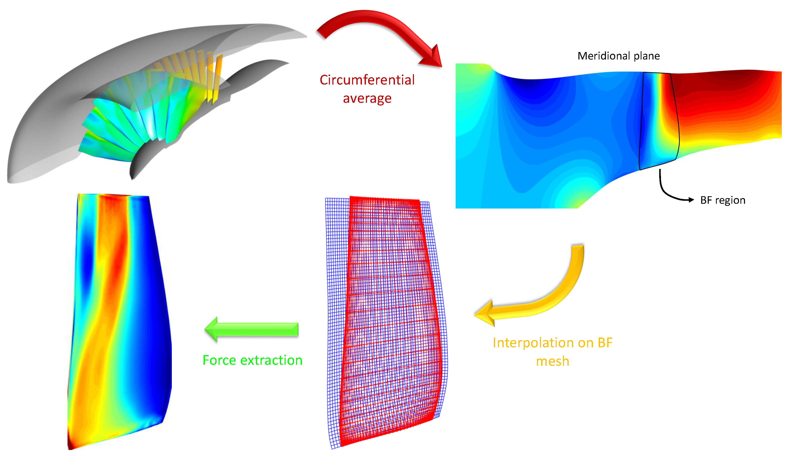
2.2. Force Reconstruction
Figure 2 summarises the workflow developed to obtain the force distribution on the blade and consequently the model input parameters. The blade is first simulated using a standard 3D single-passage steady approach. The solution is then circumferentially averaged and reduced to a bidimensional field on the meridional plane, whose support is a background mesh. In our implementation, a pre-processing module automatically computes the required blade geometric features and smoothly interpolates them from the background to the meridional body force mesh. The blade forces are isolated from the source terms of Equation (1), and finally, the model equations are inverted locally to obtain the unknown calibration fields. This procedure is only employed in the blade region, i.e., no force is applied in the tip clearance.
In the BFM solution, conversely, and are calculated on a local basis and supplied to the flow solver as source terms. Such decomposition comes from the 2D airfoil cascade theory, and in a three-dimensional solution, the parallel direction is uniquely defined, but the normal is not. The radial component can be set using the lean angle as tan(lean) [16,38], as in the original L/D version. However, this decomposition alters the total force magnitude.
In our implementation, is treated as a three-dimensional vector and applied normally to W on a plane that is also normal to the local camber surface, preserving the modulus given by Equation (3). The side of the normal is determined from the sign of , and the turning force points towards the blade concavity when positive to curve the streamlines.
With the calibration coefficients computed from the force reconstruction approach, the BFM has an explicit form that can be supplied as a source term in the balance. In our research, we developed a stand-alone tool to study throughflow methods for compressors that is called ANTARES (A Navier–Stokes Tool for Axisymmetric Rapid Engine Simulation). The flow solver employs an unstructured cell-centred second-order finite volume approximation and explicit time stepping. A high-resolution limiter is employed for convective fluxes [41], reconstructed via Roe [42] or HLLC [43] Riemann solvers. Diffusive fluxes are computed via a corrected centred approach [44] with least-square gradient reconstruction [45]. Local time-stepping and implicit residual smoothing are used for steady-state acceleration. RANS axisymmetric BFM simulations used the Spalart–Allmaras turbulence model [46,47].
2.3. Validation Test Case
The L/D model of Thollet implemented in ANTARES was validated for the NASA/GEAE R4 transonic fan rotor. This geometry represents a modern high-bypass fan design that has been studied in a large series of experiments for the source diagnostic test (STD) aeroacoustic programme collecting a valuable set of wind tunnel data [48,49,50]. The same configuration has been used by other authors, and in particular by Thollet to develop its BFM [16], allowing for a direct comparison. The rotor and outlet guide vanes (OGV) characteristics are summarised in Table 1.
In order to obtain the reference 3D solutions to be post-processed to extract the circumferential-averaged flow field and the force distribution, a CFD model for the NASA R4 turbofan was first validated. The analyses were carried out using the commercial software ANSYS CFX [51], a node-centred finite volume solver with shape function solution reconstruction. The blades were meshed with a structured multi-block topology. A sample grid of the ducted rotor case is shown in Figure 3. The mesh selection was derived from a sensitivity study on its size based on three levels of refinement using the grid convergence index (GCI) [52] to monitor the convergence of performance metrics. All the finest grids with 2.7M nodes per passage was used to simulate the fan, having a on the isentropic efficiency. It featured a resolved boundary layer with and a wall-normal growth rate below 1.16. Solutions were obtained with the Spalart–Allmaras turbulence model [46] using second-order flux reconstruction with a high-resolution Barth and Jespersen [53] limiter for advective terms.
The characteristic maps obtained with the CFD for the rotor alone configuration at the design rotational speed are shown in Figure 4 together with the NASA 9×15 ft wind tunnel data. The abscissa indicates the mass flow rate normalised with the design value . The CFD is able to adequately duplicate the experimental curves, with a close agreement of isentropic efficiency and a slightly underpredicted total pressure ratio (TPR) towards the stall.
The simulation of the complete fan with OGV stage is compared with experimental data in Figure 5. The rotor maps in Figure 5a show that the TPR is predicted with an almost constant –1% value, whereas at a lower mass flow rate, a 0.5% positive offset of efficiency is present. Downstream of the OGVs, Figure 5b, is conversely 1% higher than in experiments, whereas a smaller error in TPR is present at design mass flow. The reason for such discrepancies is attributed to slightly different inflow profiles generated by the experimental inlet that were not reproduced in the ducted computational configuration.
Among wind tunnel experiments, in fact, the stage was tested when installed in a flight model nacelle exposed to a freestream flow. The same condition was replicated in the numerics, simulating a single point at take-off, for which spanwise profiles and laser Doppler velocimetry (LDV) data had been collected. Table 2 summarizes the simulation and wind tunnel data, showing a close agreement for all reported parameters.
The circumferential-averaged spanwise profiles of total pressure, total temperature, and isentropic efficiency downstream of the rotor blade for this operating point are depicted in Figure 6 for the CFD and two wind tunnel data, collected in the NASA 9×15 ft and W8 facilities using total pressure and total temperature rakes. Figure 6a proves a good match to the experimental profile for both datasets. The reported experimental uncertainties for the W8 tunnel are on pressure rise and on adiabatic efficiency. The numerical isentropic efficiency distribution in Figure 6b falls within the uncertainty band, confirming a sufficiently accurate estimation.
The shock structure on a constant radius section at 89% of the span is illustrated in Figure 7. The experimental visualisation based on laser Doppler velocimetry (LDV) presents a detached bow shock that emanates normally along the passage from the suction side at mid chord and is curved in front of the next blade’s leading edge. The maximum Mach number of about 1.35 is reached after the suction side expansion from the leading edge. The shock structure is reproduced in the CFD, with the bow shock stand-off and the passage shock impingement location close to the experimental one. Overall, the combination of global and local quantities in the comparison validates the CFD method for the single-passage simulations that were used as a data source to build the body force model.
3. Results
The BFM implemented in ANTARES for the NASA/GEAE R4 fan is here discussed, presenting the correspondence with the reference CFD data at different operating points along the design speedline. In the comparison, the evolution of local flow quantities along the blade region is assessed for the circumferential-averaged 3D field and the axisymmetric BFM prediction. Ideally, these two solutions should be equal, but in practice, they differ due t possible data loss or errors introduced in the interpolation and averaging procedures and the lack of higher-order terms accounting for turbulent mixing and aerodynamic blockage.
3.1. Peak Efficiency Calibration Point
The first analysis was conducted at peak efficiency, which is the calibration point where the unknown fields , , and are extracted. The agreement between the BFM and the averaged CFD indicates the validity of the force extraction and inclusion of the source terms into the flow solver. Figure 8a depicts the blade contours of axial velocity. The spatial distributions are a good match, with only a slightly higher acceleration before the smeared shock predicted by the BFM. This could be due to insufficient blockage, as only the metal one is modelled, but the boundary layer growth caused by the impinging shock, that produces aerodynamic blockage, is only partially included as a deviation effect on the factor but not as a true reduction of the flow capacity. The radial velocity field, depicted in Figure 8b, also presents very similar features that were obtained thanks to the three-dimensional normal force decomposition, giving a more consistent result compared to setting the radial component as .
The absolute circumferential velocity is illustrated in Figure 9a, whereas the relative flow angle is shown in Figure 9b. The absolute tangential velocity turning is an indicator of work input and is correctly applied in the BFM. The tip and hub trailing edge corner structures are clearly visible in the body force swirl velocity contours. The close prediction of is very important in order to supply the flow with the correct force magnitude, as the model equations are heavily based on this flow parameter. This makes sure that most aerodynamic and thermodynamic variables can be accurately reproduced across the blade region.
Overall, the blade flow quantities so far compared prove that the L/D model was able to reproduce quite accurately the circumferential-averaged flow field obtained from the single-passage 3D CFD simulation in the calibration point. It is also important, however, to examine the bulk effect and in particular the distributions downstream of the cascade that contain the full history of the external work applied to the fluid by the rotating blades through the body forces. The spanwise profiles of TPR and TTR downstream of the rotor blade are reported in Figure 10. The curves are well overlapped with the reference solution and show that they qualitatively replicate endwall phenomena. At the tip, TTR is overpredicted as a result of excessive flow turning and higher work input. The efficiency profile of Figure 10b confirms a good point-to-point correspondence far from the endwalls. Here, its value is overestimated over a portion close to the hub where the CFD losses are higher.
3.2. Off-Design Performance
After validating the implementation and the model capabilities at the peak efficiency calibration point, the off-design performance was assessed. In its derivation, Thollet found that despite the use of a metal blockage, its L/D model overpredicts the choking mass flow rate due to an excessive normal force magnitude variation. As a remediation, he proposed to modify the normal force coefficient according to the rule:
where is the streamwise coordinate going from 0 at the leading edge to 1 at the trailing edge. The linear term therefore reduces the difference and thus the normal force in the first part of the blade. The offset constant must be found in order to match the choking mass flow rate. This modified version of the BFM will be referred to as calibrated, as opposed to the baseline, i.e., without the modification.
Figure 11 illustrates the characteristic maps for the NASA R4 rotor-alone case obtained with the baseline and the calibrated body force model. Without the normal force modification, the total temperature and total pressure are slightly overpredicted at the peak efficiency point, whilst the efficiency is quite close. Conversely, the choking mass flow rate is 3% larger than the CFD calculation. The calibration procedure greatly improves the choking flow rate matching and brings the TTR and TPR closer to the reference curves and the experimental points. However, a known drawback is that the efficiency curve is shifted vertically by around 2%.
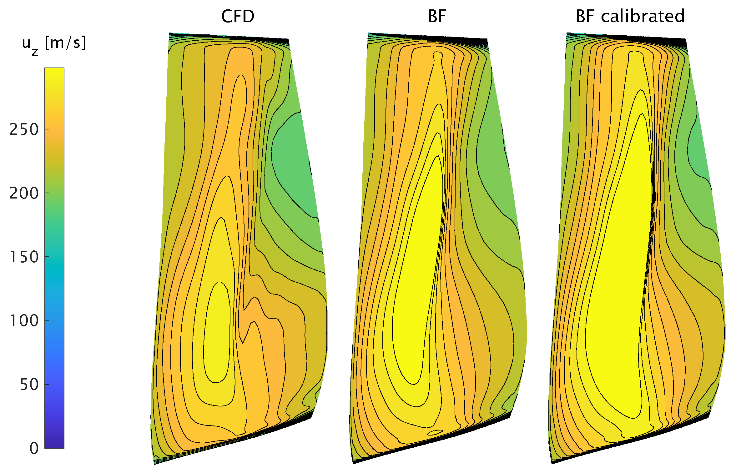
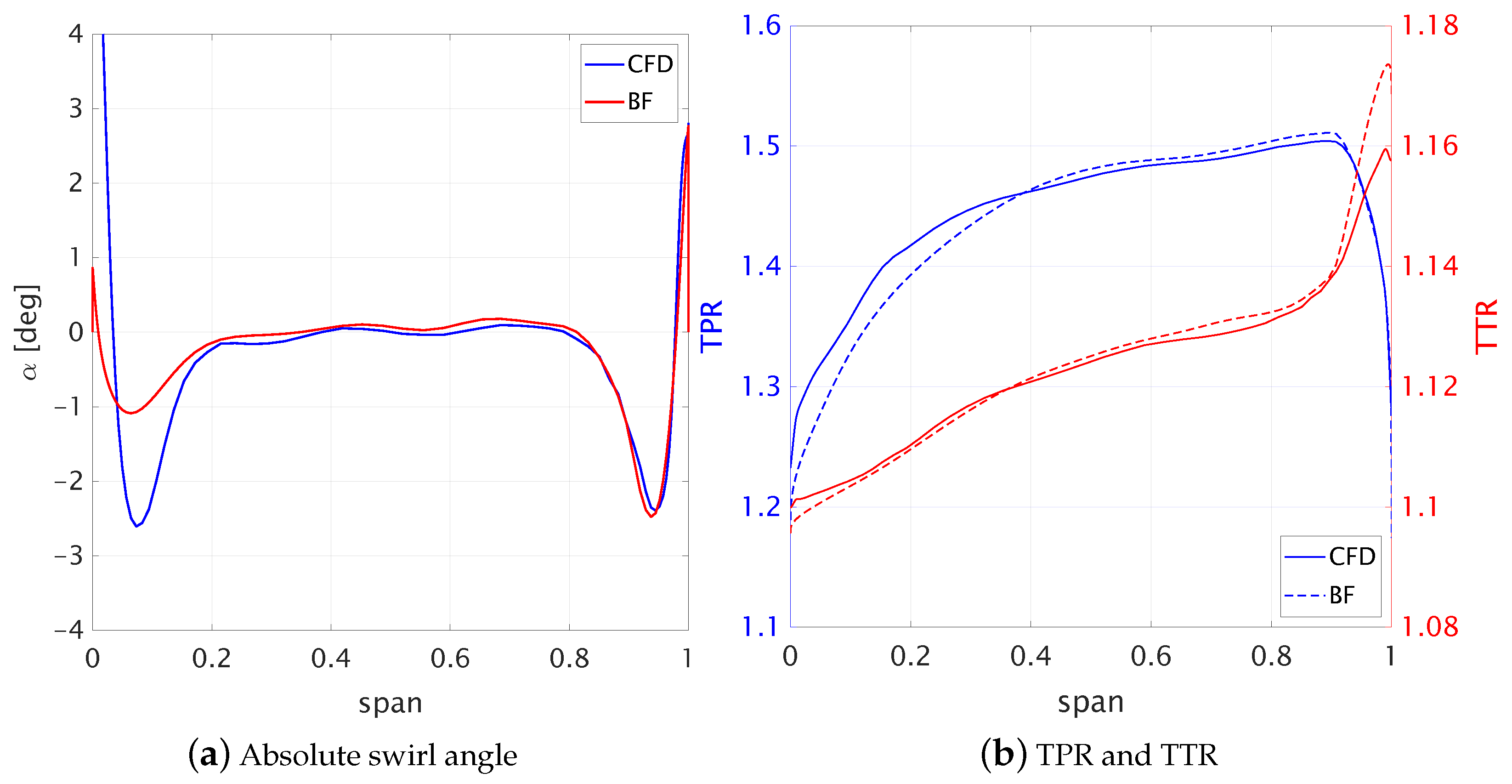
The choking mass flow calibration, despite improving the prediction of the integral characteristic parameters, alters the original force distribution over the blade along the entire speedline, thus also changing the work input and the losses introduced. Figure 12 illustrates the blade contour of the axial velocity near the choke for the reference CFD solution, the baseline, and the calibrated body force model. The smeared shock in the BF solution has a higher intensity compared to the CFD, especially at mid-span, and the resulting exit velocity is larger. The normal force calibration further magnifies the shock strength, with a larger velocity jump past mid-chord, where the shock appears, and a reduced exit velocity. The net effect is a lower axial momentum that amounts to a decreased mass flow rate. However, the correspondence occurs only in integral terms. Figure 13a reports the spanwise distribution of absolute () and relative () swirl angles downstream of the rotor, indicating an offset of around in above 50% of the span and a larger overturning near the tip, with a slight effect of the choking calibration that is more evident in the near-tip distribution. The TPR profile of Figure 13b highlights a large overprediction of the total pressure rise from 40% to 95% of the span, with a worsening near the tip after the calibration. A similar effect appears in the efficiency curve that replicates only qualitatively the reference solution but overestimates the tip region losses.
Opposite to the choking condition is the near-stall point. The characteristic maps of Figure 11 indicate that the body force model overpredicts the TTR and TPR curves slope towards the stall, regardless of the choke calibration. Figure 14a reports the absolute tangential velocity contours for the CFD and the calibrated BF model. In the first, a large tip structure trace is evident, with a high tangential velocity region that is not present in the latter. The BF values at the trailing edge are shifted towards the tip compared to the reference solution, but the profile is generally similar. The total pressure ratio distribution in Figure 14b presents an analogous behaviour, with a qualitative agreement but a larger compression for the BFM above 80% of the span.
Constant span cuts of work coefficient , shown in Figure 15a, further reveal a consistent streamwise variation predicted by the BFM. The work coefficient in the first 50% of the chord at 90% of the span is lower than the CFD, showing a kink that is not found in the BF, where the exit value is slightly larger for all span sections. The relative tangential velocity distribution at the same locations, Figure 15b, confirms a good match of the flow angles, seen also in the previous working points analysed.
Spanwise profiles downstream of rotor blade are depicted in Figure 16. The total pressure ratio of Figure 15a presents a close match up to the mid-span, apart from a local minimum near 5% of the span coming from the peak efficiency force distribution and lost in the CFD solution. On the upper half of the blade, the total pressure shape is almost linearly offset until reaching a peak, despite having a greater value that occurs in the correct position. The total temperature profile, in the same figure, is less close and smoother than the CFD one, with a good match in the tip region. The TPR and TTR discrepancies are well visible on the isentropic efficiency profile of Figure 15b. The shape differs from the CFD, and also its integral falls slightly below, as already reported in the maps of Figure 11b.
Overall, also at near-stall, some flow parameters are captured in both shape and magnitude on a region of the blade, such as the flow angles and the work coefficient, whilst other are only approximately reproduced. It must be considered that either the choke calibration somehow arbitrarily alters the force distribution, affecting the leading-to-trailing -edge evolution of the flow, and it is unlikely that the body force model is able to closely capture the force change from peak efficiency to this troublesome operating point, where the tip treatment is also likely to have an influence.
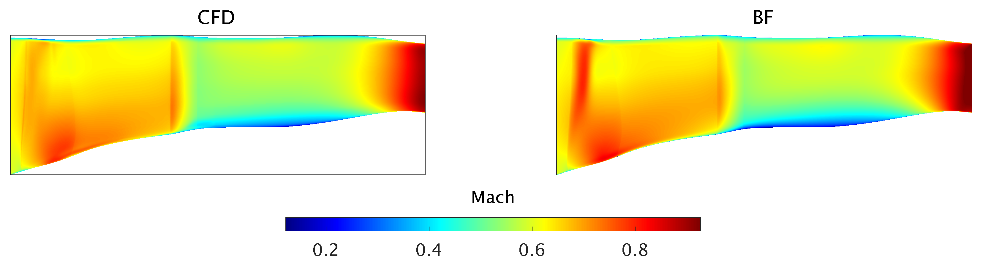
A general overview of the axisymmetric BFM flow field for the rotor alone compared to the circumferential averaged CFD solution across the speedline is presented in Figure 17 in terms of absolute Mach number. At peak efficiency and choking, the smeared shock wave is strengthened in the BFM by the normal force modification, especially at the highest mass flow, where the spanwise profiles downstream of the blade are also not closely matched. At near-stall, the CFD averaged solution features a shock region close to the leading edge, which is absent in the BFM. The outflow distribution, as in the peak efficiency point, appears to be better reproduced.
The sensitivity of the body force model to an axisymmetric change of inflow conditions was also assessed by imposing a pre-swirl of +5° and −5° to the incoming flow. Table 3 summarizes the performance index results obtained near the design point. A negative swirl drives the fan towards the stall due to an increased incidence, and vice versa, a positive swirl generates a lower incidence and shifts the operating point towards choking. The difference between the BFM and CFD is of the same magnitude as for the axial inflow case previously described for the positive swirl, while a larger discrepancy is found for the negative swirl, especially in terms of isentropic efficiency. A closer inspection of the results reveals that local deviations persist in terms of outflow profiles. Figure 18 compares the spanwise distribution of the flow and work coefficient downstream of the rotor blade between the CFD and BFM solution. Confirming the integral results, the flow coefficient is better captured for a positive swirl, whilst for the negative swirl, a higher velocity region is found between 80% and 90% of the span. In both cases, the work coefficient is overpredicted in the upper half of the blade, with a noticeable overshoot on the tip.
3.3. Fan+OGV Stage
As a final comparison case, the body force model previously described was built for the complete fan with OGV stage. The same procedure developed for the rotor was applied to the stator, i.e., extracting force data from the minimum loss point of 3D single-passage row simulations to obtain the calibration coefficients. The only difference involved the normal force modification, which was used only for the rotor.
The engine was simulated with a choked nozzle to reproduce a cruise condition. The single-point operation Mach number is depicted in Figure 19, where a similar distribution for the two models can be appreciated. The local differences in the fan blade are due to the normal force modification already discussed. In the stator blade region, the CFD circumferential-averaged solution highlights the presence of hub corner separation at the trailing edge, seen by the sudden growth of the low-Mach region on the endwall before the blade exit. The velocity deficit begins in the second part of the chord at low span and continues downstream, up to the nozzle restriction where the flow reacquires its full velocity distribution. This feature is also present in the BFM field, although with a different development. In fact, it originates earlier and has a higher thickness. By examining the angle distribution downstream of the OGVs, shown in Figure 20a, it can be noticed that the stator has a large underturning near the endwalls, with a residual swirl of about . Whilst the tip underturning is well-matched by the BF model, the hub is not as a consequence of a lower axial and circumferential velocity, with the difference in being up to . The effect of this behaviour can also be seen in the TPR and TTR profiles downstream of the OGV, reported in Figure 20b. At up to 40% of the span, the total pressure predicted by the BFM is below the reference solution of about 2.5% in absolute value, whilst it is slightly above at a higher span. Overall, the curve shape is well-replicated. The situation for the TTR, entirely depending on the rotor, is symmetric, with the tip overshoot already seen.
In terms of integral quantities, the single-point operation results are summarised in Table 4. The mass flow rate predicted by the BF computation is 0.2% higher relative to the CFD calculation. TPR and TTR are also closely matched. However, the slight difference results in an efficiency underprediction by 1.4% in absolute terms.
3.4. Installed Engine Operation
In this section, an applicative example of the use of the BFM to study fan/airframe interactions is presented. As outlined in the introduction, a purpose of these methods is to enable coupled flow simulations where the interaction is modelled in a physically consistent way, as opposed to decoupled approaches. In the latter, the fan operates irrespectively of the flow past the inlet and exhaust, which can lead to inaccurate prediction of aeropropulsive performance at severe off-design conditions or in tightly integrated configurations. In this example, an isolated nacelle of an ultra-high bypass ratio turbofan is simulated using a boundary conditions (B/C)-based approach and a BFM representation of the fan with the OGV stage. The two models are compared at take-off with and an angle of attack and . In the B/C solution, the fan face was represented as a mass flow outlet, and the bypass and core nozzle inlet planes as pressure inflows, with stagnation parameters specified. The domain included the complete turbofan with a nacelle cowl, exhaust, and pylon and the freestream region delimited by a farfield boundary. The BFM was implemented in the commercial software Ansys Fluent [54] to solve the three-dimensional problem. For the B/C, only half of the domain was simulated, exploiting the geometric symmetry, whereas the full shape was needed for the BFM due to the non-axisymmetric engine response. Further details of the computational set-up are given in [55], where different nacelle geometries are examined. Here, the focus is on illustrating the different solutions obtained with a standard and a flow-coupled approach.
At , the Mach number distributions reported in Figure 21a appear well-resembling. The flow past the external cowl is duplicated by the inlet mass flow matching. The moderate incidence allows for an attached flow over the intake. On the exhaust, the stage radial profiles in the BFM respond to the inflow and outflow conditions, producing an uneven distribution of stagnation parameters. Despite the apparent goodness of the kinematic similitude, the net thrust delivered by the turbofan was measured to be 2.18% higher in the B/C relative to the BFM as a result of a slightly different wall force distribution. In fact, the match occurred only on average, since the inflow and outflow parameters were specified as even fields. When facing a more severe condition beyond the maximum wing at , Figure 21b illustrates a totally different situation: the intake was deeply stalled in the B/C, whereas the flow remained attached in the BFM. It is well known, in fact, that the effect of the fan is to react to a nonuniform incoming pressure field and impose an upstream flow redistribution attenuating the lip separation.
In the B/C model, the mass flow at the fan inlet is set as a boundary condition. Therefore, it is equally achieved for a converged simulation regardless of the incoming distribution. This means that the upper part of the fan inlet receives a huge mass flux to compensate for the detachment on the lower part, giving rise to a much higher velocity inside the inlet duct. Equivalently, the discharged flow is insensitive to the fact that the rotor is operating with a prohibitive distortion, and the stagnation parameters remain the same as the previous angle of attack.
In the BFM simulation, the solution is fully coupled between the fan stage and the airframe flow, and no separation is produced on the lip. Both the static pressure at the fan face and the distribution of the stagnation parameters and velocity on the bypass nozzle inlet are the result of this coupling, where the final mass flow depends on the equilibrium point reached along the iso-speed characteristic curve. In fact, despite the degraded flow in the B/C, the predicted net thrust was 8.95% higher than the BFM. The reason is that as increased, all boundary values remained unchanged as if the engine were operating in a clean condition; therefore, the mass flow did not reduce, the nozzle continued to produce the nominal thrust, and the intake stall altered the surface forces.
The example clearly demonstrates that when the physical interaction of the airframe and the propulsor becomes relevant, traditional approaches can provide deceptive, yet convergent, solutions that are likely to give rise to noticeable errors on the prediction of the aerodynamic and propulsive performance.
4. Conclusions
The lift/drag body force model has been implemented into the developed computational tool ANTARES and investigated for the NASA R4 transonic fan. Through a systematic comparison of the BFM predictions with the circumferential-averaged solution from validated 3D CFD simulations, several features of the model have been highlighted. The good match achieved with the baseline version at the peak efficiency point in terms of local and global predictions proves the validity of the calibration procedure and the force application.
The analysis of performance metrics along the speedline after the application of the choking mass flow rate modification shows a good representation of the total pressure rise characteristic, with a 0.6% absolute difference at peak efficiency and a moderately larger slope towards the stall. On the contrary, the isentropic efficiency was penalised, resulting in an almost constant error close to −2%, despite a consistent curve shape.
The procedure of altering the normal force to match the choking mass flow is an evident weakness of the model, but it is necessary to restore a satisfactory integral agreement. This occurs at the expense of a less precise local correspondence. Because of this and the dependency upon local calibration coefficients that are a function of the blade geometry, the model appears to be suitable for analysis purposes only. On the other hand, even with this limitation, it has shown to be able to provide a sufficiently accurate flow field with a good resolution of the spanwise distributions, particularly for lower-than-designed mass flow rates. Local higher discrepancies have been highlighted in the endwall regions that are more sensitive to the force application due to the presence of the boundary layer and secondary flows, especially in the tip area, where, in general, an enthalpy rise overshoot was present.
Overall, the model appears to be a suitable tool to generate middle-fidelity simulations without the cost of URANS. Despite its limitations in providing an accurate estimation of the efficiency level and the presence of some larger errors in the outflow profiles close to the endwalls, the body force solution reaches the consistent equilibrium point where the engine is driven to work as a result of the full coupling between the inlet, the engine, and the nozzle flow. Therefore, it achieves a substantial improvement and a much more physics-based representation compared to classic decoupled approaches, such as the boundary conditions-based method described for the powered nacelle, that are only valid for a truly independent operation of the propulsor components.
Funding
Part of this research was conducted within the Clean Sky 2 project IVANHOE (Installed adVAnced Nacelle uHbr Optimisation and Evaluation), funded by the European Union’s Horizon 2020 research and innovation programme under the grant agreement number 863415.
Data Availability Statement
Not applicable.
Conflicts of Interest
The author declares no conflict of interest.
Nomenclature
The following abbreviations are used in this manuscript:
| BFM | Body force model |
| CFD | Computational fluid dynamics |
| OGV | Outlet guide vanes |
| RANS | Reynolds-averaged Navier–Stokes |
| SLC | Streamline curvature |
| TPR | Total pressure ratio |
| TTR | Total temperature ratio |
| Absolute circumferential flow angle, angle of attack | |
| Relative circumferential flow angle | |
| b | Blade metal blockage |
| c | Blade chord |
| Isentropic efficiency | |
| e | Specific total energy |
| Normal force | |
| Parallel force | |
| M | Mach number |
| Mass flow rate | |
| dynamic viscosity | |
| p | Static pressure |
| Total pressure | |
| r | Radial direction |
| Circumferential direction | |
| Density | |
| T | Static temperature |
| Blade maximum thickness | |
| Conservative variable vector | |
| u | Absolute velocity |
| w | Relative velocity |
| Flow coefficient | |
| Work coefficient | |
| z | Axial direction |
| Z | Number of cascade blades |
| Rotational speed |
Appendix A
The BFM solution in ANTARES is obtained by solving the following axisymmetric Navier-Stokes equations:
where is the conservative variable vector. , are the convective fluxes along the axial and radial direction and , are the diffusive fluxes along the same respective directions. Several source terms appear:
and come from the application of the divergence theorem in cylindrical coordinates. is the rotational speed of the machine. and are the body forces representing the effect of the blades on the fluid, whose expression depends on the model employed. b is the metal blockage parameter.
References
- IATA. Aircraft Technology Roadmap to 2050; Report; IATA: Geneva, Switzerland, 2019. [Google Scholar]
- NLR; Economics, S.A. Destination 2050—A Route to Net Zero European Aviation; Report NLR-CR-2020-510; NLR—Royal Netherlands Aerospace Centre: Amsterdam, The Netherlands, 2021. [Google Scholar]
- Nickol, C.L.; Haller, W.J. Assessment of the performance potential of advanced subsonic transport concepts for NASA’s Eenvironmentally responsible aviation project. In Proceedings of the 54th AIAA Aerospace Sciences Meeting, San Diego, CA, USA, 4–8 January 2016; AIAA: Reston, VI, USA, 2016. [Google Scholar] [CrossRef] [Green Version]
- Carrier, G. Innovative engine integration solutions for transport aircraft: Current research and future challenges. Presented at the EUCASS 2017, Milano, Italy, 6 July 2017; EUCASS: Bruxelles, Belgium, 2017. [Google Scholar]
- Menegozzo, L.; Benini, E. Boundary Layer Ingestion Propulsion: A Review on Numerical Modeling. J. Eng. Gas Turbines Power 2020, 142, 120801. [Google Scholar] [CrossRef]
- Magrini, A.; Benini, E.; Yao, H.D.; Postma, J.; Sheaf, C. A review of installation effects of ultra-high bypass ratio engines. Prog. Aerosp. Sci. 2020, 119, 100680. [Google Scholar] [CrossRef]
- Hendricks, E.S. A Review of Boundary Layer Ingestion Modeling Approaches for Use in Conceptual Design; Report, NASA/TM—2018-219926; NASA: Washington, DC, USA, 2018.
- Gong, Y. A Computational Model for Rotating Stall and Inlet Distortions in Multistage Compressors. Ph.D. Thesis, Massachussets Institute of Technology, Cambridge, MA, USA, 1999. [Google Scholar]
- Peters, A. Ultra-Short Nacelles for Low Fan Pressure Ratio Propulsors. Ph.D. Thesis, Massachusetts Institute of Technology, Cambridge, MA, USA, 2014. [Google Scholar]
- Peters, A.; Spakovszky, Z.S.; Lord, W.K.; Rose, B. Ultrashort Nacelles for Low Fan Pressure Ratio Propulsors. J. Turbomach. 2014, 137, 21001. [Google Scholar] [CrossRef] [Green Version]
- Hall, D.K. Analysis of Civil Aircraft Propulsors with Boundary Layer Ingestion. Ph.D. Thesis, Massachusetts Institute of Technology, Cambridge, MA, USA, 2015. [Google Scholar]
- Hall, D.K.; Greitzer, E.M.; Tan, C.S. Analysis of fan stage conceptual design attributes for boundary layer ingestion. J. Turbomach. 2017, 139, 071012. [Google Scholar] [CrossRef] [Green Version]
- Akaydin, H.D.; Pandya, S.A. Implementation of a body force model in OVERFLOW for propulsor simulations. In Proceedings of the 35th AIAA Applied Aerodynamics Conference, Denver, CO, USA, 5–9 June 2017; American Institute of Aeronautics and Astronautics: Reston, VI, USA, 2017. [Google Scholar] [CrossRef] [Green Version]
- Thollet, W.; Dufour, G.; Carbonneau, X.; Blanc, F. Body-force modeling for aerodynamic analysis of air intake—Fan interactions. Int. J. Numer. Methods Heat Fluid Flow 2016, 26, 2048–2065. [Google Scholar] [CrossRef] [Green Version]
- Thollet, W.; Dufour, G.; Carbonneau, X.; Blanc, F. Assessment of body force methodologies for the analysis of intake-fan aerodynamic interactions. In Proceedings of the ASME Turbo Expo, Seoul, Republic of Korea, 13–17 June 2016. [Google Scholar] [CrossRef]
- Thollet, W. Body Force Modeling of Fan-Airframe Interactions. Ph.D. Thesis, Université de Tolouse—ISAE, Tolouse, France, 2017. [Google Scholar]
- Benichou, E.; Dufour, G.; Bousquet, Y.; Binder, N.; Ortolan, A.; Carbonneau, X. Body Force Modeling of the Aerodynamics of a Low-Speed Fan under Distorted Inflow. Int. J. Turbomach. Propuls. Power 2019, 4, 29. [Google Scholar] [CrossRef] [Green Version]
- Awes, A.; Dufour, G.; Daon, R.; Marty, J.; Barrier, R.; Carbonneau, X. Unsteady body force methodology for fan operability assessment under clean and distorted inflow conditions. In Proceedings of the AIAA Scitech 2021 Forum, Virtual, 11–15 January 2021; AIAA: Reston, VI, USA, 2021. [Google Scholar] [CrossRef]
- Godard, B.; Ben Nasr, N.; Barrier, R.; Marty, J.; Gourdain, N.; De Jaeghere, E. Methodologies for turbofan inlet aerodynamics prediction. In Proceedings of the 35th AIAA Applied Aerodynamics Conference, Denver, CO, USA, 5–9 June 2017; American Institute of Aeronautics and Astronautics: Reston, VI, USA, 2017. [Google Scholar] [CrossRef]
- Magrini, A.; Buosi, D.; Benini, E. Sensitivity analysis of nacelle intake high-incidence aerodynamics including a body force fan model. In Proceedings of the AIAA Scitech 2021 Forum, Virtual, 11–15 January 2021; AIAA: Reston, VA, USA, 2021. [Google Scholar] [CrossRef]
- Magrini, A.; Benini, E.; Buosi, D. Design of short intakes for ultra-high bypass engines: Preliminary exploration at fixed incidence. In Proceedings of the AIAA Scitech 2022 Forum, San Diego, CA, USA, 3–7 January 2022; AIAA: Reston, VA, USA, 2022. [Google Scholar] [CrossRef]
- Magrini, A.; Benini, E. Study of geometric parameters for the design of short intakes with fan modelling. Chin. J. Aeronaut. 2022, in press. [Google Scholar] [CrossRef]
- Magrini, A.; Buosi, D.; Benini, E. Assessment of engine modelling on the installed aerodynamics of an ultra-high bypass turbofan. In Proceedings of the AIAA Scitech 2022 Forum, San Diego, CA, USA, 3–7 January 2022; AIAA: Reston, VA, USA, 2022. [Google Scholar] [CrossRef]
- Chima, R.V.; Arend, D.J.; Castner, R.S.; Slater, J.W.; Truax, P.P. CFD models of a serpentine inlet, fan, and nozzle. In Proceedings of the 48th AIAA Aerospace Sciences Meeting Including the New Horizons Forum and Aerospace Exposition, Orlando, FL, USA, 4–7 January 2010; American Institute of Aeronautics and Astronautics: Reston, VI, USA, 2010. [Google Scholar] [CrossRef]
- Guo, J.; Hu, J. A three-dimensional computational model for inlet distortion in fan and compressor. Proc. Inst. Mech. Eng. Part A J. Power Energy 2018, 232, 144–156. [Google Scholar] [CrossRef]
- Hill, D.J.; Defoe, J.J. Innovations in Body Force Modeling of Transonic Compressor Blade Rows. Int. J. Rotating Mach. 2018, 2018, 6398501. [Google Scholar] [CrossRef]
- Mao, Y.; Dang, T.Q. A three-dimensional body-force model for nacelle-fan systems under inlet distortions. Aerosp. Sci. Technol. 2020, 106, 106085. [Google Scholar] [CrossRef]
- Pazireh, S.; Defoe, J.J. A New Loss Generation Body Force Model for Fan/Compressor Blade Rows: An Artificial-Neural-Network Based Methodology. Int. J. Turbomach. Propuls. Power 2021, 6, 5. [Google Scholar] [CrossRef]
- Cao, T.; Hield, P.; Tucker, P.G. Hierarchical immersed boundary method with smeared geometry. J. Propuls. Power 2017, 33, 1151–1163. [Google Scholar] [CrossRef]
- Cui, J.; Watson, R.; Ma, Y.; Tucker, P. Low order modeling for fan and outlet guide vanes in aero-engines. J. Turbomach. 2019, 141, 031002. [Google Scholar] [CrossRef] [Green Version]
- Burlot, A.; Sartor, F.; Vergez, M.; Méheut, M.; Barrier, R. Method comparison for fan performance in short intake nacelle. In Proceedings of the 2018 Applied Aerodynamics Conference, Atlanta, GA, USA, 25–29 June 2018; American Institute of Aeronautics and Astronautics: Reston, VI, USA, 2018. [Google Scholar] [CrossRef]
- Ma, Y.; Vadlamani, N.R.; Cui, J.; Tucker, P. Comparative studies of RANS versus large eddy simulation for fan-intake interaction. J. Fluids Eng. Trans. ASME 2019, 141, 031106. [Google Scholar] [CrossRef]
- Godard, B.; de Jaeghere, E.; Gourdain, N. Efficient design investigation of a turbofan in distorted inlet conditions. In Proceedings of the ASME Turbo Expo, Phoenix, AZ, USA, 17–21 June 2019; American Society of Mechanical Engineers (ASME): New York, NY, USA, 2019; Volume 2A-2019. [Google Scholar] [CrossRef] [Green Version]
- Adamczyk, J. Model Equation for Simulating Flows in Multistage Turbomachinery; Technical Report; NASA: Washington, DC, USA, 1984.
- Baralon, S.; Eriksson, L.E.; Hall, U. Evaluation of higher-order terms in the throughflow approximation using 3D Navier-Stokes computations of a transonic compressor rotor. In Proceedings of the Turbo Expo: Power for Land, Sea, and Air, Indianapolis, IN, USA, 7–10 June 1999; Volume 1. [Google Scholar] [CrossRef] [Green Version]
- Simon, J.; Thomas, J.P.; Léonard, O. On the Role of the Deterministic and Circumferential Stresses in Throughflow Calculations. J. Turbomach. 2009, 131, 031019. [Google Scholar] [CrossRef]
- Baralon, S.; Eriksson, L.E.; Håll, U. Validation of a throughflow time-marching finite-volume solver for transonic compressors. In Proceedings of the International Gas Turbine and Aeroengine Congress and Exhibition, Stockholm, Sweden, 2–5 June 1998. [Google Scholar] [CrossRef] [Green Version]
- Simon, J.F. Contribution to Throughflow Modelling for Axial Flow Turbomachine. Ph.D. Thesis, Université de Liège, Liège, Belgium, 2007. [Google Scholar]
- Magrini, A. Study of Body Force Modelling for Coupled Fan/Airframe Simulations. Ph.D. Thesis, Università Degli Studi di Padova, Padova, Italy, 2020. [Google Scholar]
- Marble, F. Three dimensional flow in turbomachines. In Volume X of High Speed Aerodynamics and Jet Propulsion; Hawthorne, W.R., Ed.; Princeton University Press: Princeton, NJ, USA, 1964. [Google Scholar]
- Tsoutsanis, P. Extended bounds limiter for high-order finite-volume schemes on unstructured meshes. J. Comput. Phys. 2018, 362, 69–94. [Google Scholar] [CrossRef]
- Roe, P.L.; Pike, J. Efficient construction and utilisation of approximate Riemann solutions. In Proceedings of the 6th International Symposium on Computing Methods in Applied Sciences and Engineering, VI, Versailles, France, 12–16 December 1983; North-Holland Publishing Co.: Amsterdam, The Netherlands, 1985; pp. 499–518. [Google Scholar]
- Toro, E.F. Riemann Solvers and Numerical Methods for Fluid Dynamics: A Practical Introduction; Springer: Berlin/Heidelberg, Germany, 2009; pp. 1–724. [Google Scholar] [CrossRef]
- Jalali, A.; Ollivier Gooch, C.F. Higher-order finite volume solution reconstruction on highly anisotropic meshes. In Proceedings of the 21st AIAA Computational Fluid Dynamics Conference, San Diego, CA, USA, 24–27 June 2013; American Institute of Aeronautics and Astronautics: Reston, VI, USA, 2013. [Google Scholar] [CrossRef]
- Ollivier-Gooch, C.; Van Altena, M. A High-Order-Accurate Unstructured Mesh Finite-Volume Scheme for the Advection–Diffusion Equation. J. Comput. Phys. 2002, 181, 729–752. [Google Scholar] [CrossRef]
- Spalart, P.R.; Allmaras, S.R. One-equation turbulence model for aerodynamic flows. Rech. Aérosp. 1994, 1, 5–21. [Google Scholar] [CrossRef]
- Allmaras, S.R.; Johnson, F.T.; Spalart, P.R. Modifications and clarications for the implementation of the spalart-allmaras turbulence model. In Proceedings of the International Conference on Computational Fluid Dynamics, Tokyo, Japan, 9–10 January 2012. [Google Scholar]
- Podboy, G.G.; Krupar, M.J.; Hughes, C.E.; Woodward, R.P. Fan Noise Source Diagnostic Test—LDV Measured Flow Field Results; Technical Report; NASA Glenn Research Center: Cleveland, OH, USA, 2003.
- Hughes, C.E.; Jeracki, R.J.; Woodward, R.P.; Miller, C.J. Fan Noise Source Diagnostic Test—Rotor Alone Aerodynamic Performance Results; Technical Report; NASA Glenn Research Center: Cleveland, OH, USA, 2005.
- Van Zante, D.E.; Podboy, G.G.; Miller, C.J.; Thorp, S.A. Testing and Performance Verifi cation of a High Bypass Ratio Turbofan Rotor in an Internal Flow Component Test Facility; Technical Report; NASA Glenn Research Center: Cleveland, OH, USA, 2009.
- Ansys, I. ANSYS CFX-Solver Theory Guide; Ansys, Inc.: Canonsburg, PA, USA, 2018. [Google Scholar]
- ASME. Procedure for Estimation and Reporting of Uncertainty Due to Discretization in CFD Applications. J. Fluids Eng. 2008, 130, 78001. [Google Scholar] [CrossRef] [Green Version]
- Barth, T.; Jespersen, D. The design and application of upwind schemes on unstructured meshes. In Proceedings of the 27th Aerospace Sciences Meeting, Reno, NV, USA, 9–12 January 1989. [Google Scholar] [CrossRef]
- Ansys, I. ANSYS Fluent User Manual; Ansys, Inc.: Canonsburg, PA, USA, 2018. [Google Scholar]
- Magrini, A.; Buosi, D.; Benini, E. Analysis of ultra-high bypass ratio turbofan nacelle geometries with conventional and short intakes at take-off and cruise. In Proceedings of the ASME Turbo Expo 2022, Rotterdam, The Netherlands, 13–17 June 2022. [Google Scholar] [CrossRef]
Figure 1.
Blade geometric parameters and forces acting on the axisymmetric flow field. The normal component turns the streamlines, the parallel component increases entropy and adds losses.
Figure 1.
Blade geometric parameters and forces acting on the axisymmetric flow field. The normal component turns the streamlines, the parallel component increases entropy and adds losses.

Figure 2.
Force extraction work flow.

Figure 3.
Ducted rotor mesh sample.

Figure 4.
Rotor-alone characteristic maps for CFD and experiments.

Figure 5.
Fan and OGV stage characteristic maps a .

Figure 6.
Comparison of experimental and calculated circumferential-averaged spanwise profiles downstream of rotor blade for fan+OGV single-point take-off operation.
Figure 6.
Comparison of experimental and calculated circumferential-averaged spanwise profiles downstream of rotor blade for fan+OGV single-point take-off operation.

Figure 7.
Comparison of CFD and experimental relative Mach number distribution on a constant radius section 263.1 mm from the axis for single-point take-off operation.
Figure 7.
Comparison of CFD and experimental relative Mach number distribution on a constant radius section 263.1 mm from the axis for single-point take-off operation.

Figure 8.
Velocity contours on the blade for reference CFD solution and baseline body force model at peak efficiency.
Figure 8.
Velocity contours on the blade for reference CFD solution and baseline body force model at peak efficiency.

Figure 9.
Absolute circumferential velocity and relative swirl angle contours on the blade for reference CFD solution and baseline body force model at peak efficiency.
Figure 9.
Absolute circumferential velocity and relative swirl angle contours on the blade for reference CFD solution and baseline body force model at peak efficiency.

Figure 10.
Spanwise distributions downstream of rotor blade for reference CFD solution and baseline body force model at peak efficiency.
Figure 10.
Spanwise distributions downstream of rotor blade for reference CFD solution and baseline body force model at peak efficiency.

Figure 11.
Fan characteristic maps using baseline and calibrated BFM vs. CFD reference solution and experimental data.
Figure 11.
Fan characteristic maps using baseline and calibrated BFM vs. CFD reference solution and experimental data.

Figure 12.
Axial velocity contours at near-choke for reference CFD solution, baseline, and calibrated BFM.
Figure 12.
Axial velocity contours at near-choke for reference CFD solution, baseline, and calibrated BFM.

Figure 13.
Spanwise distributions downstream of rotor blade at near choke for CFD, baseline, and calibrated body force model.
Figure 13.
Spanwise distributions downstream of rotor blade at near choke for CFD, baseline, and calibrated body force model.

Figure 14.
Blade contours at near-stall for reference CFD solution and calibrated BFM.

Figure 15.
Streamwise profiles at near stall for reference CFD solution and calibrated BFM.

Figure 16.
Spanwise profiles downstream of rotor blade at near-stall for reference CFD solution and calibrated BFM.
Figure 16.
Spanwise profiles downstream of rotor blade at near-stall for reference CFD solution and calibrated BFM.

Figure 17.
Mach number contours for ducted rotor-alone case at different operating points.

Figure 18.
Spanwise distributions downstream of rotor blade of work and flow coefficient for pre-swirled flow near peak efficiency.
Figure 18.
Spanwise distributions downstream of rotor blade of work and flow coefficient for pre-swirled flow near peak efficiency.

Figure 19.
Mach number distribution for fan+OGV stage with CFD (left) and BF model (right).

Figure 20.
Outflow radial profiles for fan+OGV stage.

Figure 21.
Mach number distribution for isolated nacelle case at and two angles of attack with boundary conditions (left) and body force (right) engine modelling.
Figure 21.
Mach number distribution for isolated nacelle case at and two angles of attack with boundary conditions (left) and body force (right) engine modelling.


Table 1.
NASA/GEAE R4 characteristics.
| Fan | OGV Baseline | |
|---|---|---|
| No Blades | 22 | 54 |
| Aspect Ratio | 2.0 | 3.51 |
| Hub/Tip ratio | 0.30 | 0.50 |
| Chord (mm) | 91.694 | 39.878 |
| Solidity | 1.73 | 1.52 |
| Stagger (deg) | 37.10 | 10.29 |
| tip | 0.028 | 0.0698 |
Table 2.
NASA/GEAE R4 fixed-nozzle take-off operation. Comparison of CFD result and wind tunnel measurements.
Table 2.
NASA/GEAE R4 fixed-nozzle take-off operation. Comparison of CFD result and wind tunnel measurements.
| [kg/s] | TPR | TTR | ||
|---|---|---|---|---|
| Exp. | 44.09 | 1.511 | 1.136 | 91.7 % |
| CFD | 44.07 | 1.510 | 1.1357 | 92.1 % |
Table 3.
Swirl flow calculations near peak efficiency.
| Model | Swirl [deg] | [kg/s] | TPR | TTR | |
|---|---|---|---|---|---|
| BF | +5 | 47.465 | 1.478 | 1.133 | 0.890 |
| CFD | +5 | 47.276 | 1.474 | 1.129 | 0.906 |
| BF | −5 | 44.653 | 1.452 | 1.123 | 0.916 |
| CFD | −5 | 44.476 | 1.448 | 1.119 | 0.934 |
Table 4.
Integral performance indexes of fan+OGV stage for CFD and BFM models.
| TPR | TTR | |||
|---|---|---|---|---|
| (BFM-CFD) | 0.091 | −0.001 | 0.002 | −0.014 |
| (BFM- CFD)/CFD [%] | 0.20 | 0.068 | 0.177 | −1.55 |
Publisher’s Note: MDPI stays neutral with regard to jurisdictional claims in published maps and institutional affiliations. |
© 2022 by the author. Licensee MDPI, Basel, Switzerland. This article is an open access article distributed under the terms and conditions of the Creative Commons Attribution (CC BY) license (https://creativecommons.org/licenses/by/4.0/).
Share and Cite
MDPI and ACS Style
Magrini, A. Body Force Model Implementation of Transonic Rotor for Fan/Airframe Simulations. Aerospace 2022, 9, 725. https://doi.org/10.3390/aerospace9110725
AMA Style
Magrini A. Body Force Model Implementation of Transonic Rotor for Fan/Airframe Simulations. Aerospace. 2022; 9(11):725. https://doi.org/10.3390/aerospace9110725
Chicago/Turabian StyleMagrini, Andrea. 2022. "Body Force Model Implementation of Transonic Rotor for Fan/Airframe Simulations" Aerospace 9, no. 11: 725. https://doi.org/10.3390/aerospace9110725
Note that from the first issue of 2016, this journal uses article numbers instead of page numbers. See further details here.