1. Introduction
The steer of large-scale multi-agent particle systems is challenging due to the high degree of freedom in such distributed systems of loosely coupled robots [
1]. The published approaches on this subject can roughly be separated into two complementary classes: (A) centralized approaches assuming complete information and focusing on precision and efficiency [
2] and (B) decentralized approaches assuming only partial observability and focusing on simple reactive and behavior-based control [
3]. While both concepts are generally justified, the centralized approach may be almost unavoidable for certain tasks. Here, we investigate a control problem in robot swarms with minimal hardware [
4,
5]. In the case of a simple robot, such as the Kilobot robot with its minimal equipment of sensors [
6], certain tasks may be infeasible relying on a decentralized approach. The advantage of having simple hardware is, in turn, that possibly many robots can be built to form a large-scale formation with high redundancy. The automatic control problem can be thought of as macroscopic or stochastic control of a
cloud of robots determined by a distribution [
4,
7].
The global input can be, for example, the mean position of all robots and their variance. The output is a global control law that is broadcasted to all robots or that operates as a moment of force on each robot. The variance may be calculated based on robot positions [
5], which could be relaxed in a different approach. An option is to exploit the environment by gathering robots at flat obstacles until minimum variance is achieved [
8]. The control iterates over measuring robot positions followed by possibly longer periods of not measuring again but relying on the dynamical model of each robot plus adding Brownian noise on positions, velocities, and accelerations. This is generally related to mean-field models of multi-robot systems [
9] and, specifically, the concept of assuming microscopically Brownian particles and the resulting macroscopic evolution of a swarm described by a distribution relates directly to known modeling approaches in swarm robotics based on Langevin equations and Fokker-Planck equations [
10].
We propose an optimal energy-efficient control mechanism that minimizes positional variance and steers the robot system’s mean position to a target position. In particular, our work starts by showing that it is possible to obtain mathematically a mapping such that underactuated robot systems take a partial form. However, due to the complexity of the dynamics (coupling of the inertia matrix), it is not possible to design a controller. Another challenge is the fact that the control input matrix
is time-variant. However, in [
3,
11,
12], the authors assumed the input matrix to be in the form of
. This assumption on the input matrix
G can be applied only to simple robot structures. In this paper, we cover the case where
has a general form. Therefore, we relax this assumption on the input matrix
G differently from what is done in [
3,
11,
12]. Indeed, finding a transformation to have the robot systems take a partial form is not straightforward. Nonetheless, a new generalized coordinate transformation framework is proposed to decouple the system. This allows the development of an optimal control mechanism with the prime objective of energy efficiency. In control theory, several techniques exist to design energy-efficient control laws [
13]. However, the state-dependent Riccati equation (SDRE) [
14] does not cancel nonlinear terms, which is advantageous because canceling such nonlinearities would significantly increase the control signals [
15]. Furthermore, SDRE parameterizes and characterizes the system to a state-dependent coefficient (SDC) form that is useful for immediate stability analysis. Then, we show that our control design provides set point tracking (stabilization) with semi-global properties. Our proof is based on the Lyapunov stability criterion [
16].
Recently in [
2], the author introduced a centralized control of underactuated nonidentical Euler–Lagrange systems. The methodology is valid based on the assumption of the accessibility of the information of the whole network. In this paper, we develop a novel centralized control of underactuated large-scale multi-agent systems using only the mean position of all agents and their variance. The experiment highlights three advantages: (i) It resolves the limitation of the existing control strategy by introducing a novel two-step methodology to control the swarm, (ii) it increases the performance by exploiting the torque generated for the orientation of particles and providing smoother trajectories, and (iii) it proposes a base performance comparison with the actuated holonomic swarm of particles [
5,
17].
2. Euler-Lagrange Dynamics
We consider an underactuated robot system with dynamics described by the well-known Euler-Lagrange (EL) equations of motion
where
are the configuration variables,
are the control signals,
is the generalized inertia matrix,
represent the Coriolis and centrifugal forces,
is the systems potential energy, and
is the input matrix. First, we make an assumption characterizing the class of generalized coordinate transformation
T that we use here.
Assumption 1. There exists an invertible mapping , such thatis invertible for all q. Lemma 1. Consider a mapping that satisfies Assumption 1 and define the generalised coordinate transformation as followsThen, the EL dynamics (1) can be written as followswhereand are the Coriolis and centrifugal forces associated with mass matrix that we can compute byThe Lagrangian in the new generalized coordinates is Proof. The proof follows from the coordinate invariance property of the EL equations (or from straightforward calculation computing the derivative of the coordinate transformation and using the original dynamics). □
Remark 1. Notice that the matrix can be used to shape the form of the mass matrix in the new generalized coordinates. However, we only consider invertible matrices that satisfy the integrability Assumption 1. That is, given an invertible matrix , we assume there exists an invertible mapping that satisfiesTherefore, the generalized coordinated transformation (3) is well-defined. We consider now mechanical systems (
1) with an input matrix of the general form
where rank
, and
is an invertible
matrix.
and
are the underactuated and actuated components of
, respectively. The EL dynamics (
1) is coupled when
. Furthermore, to simplify the notation, we partition the generalized coordinates and velocity as
,
with
and
, and partition the inertia and Coriolis matrices as
where
,
,
,
,
,
,
. Next, we impose several assumptions to show particular forms of the EL dynamics (
1) under generalized coordinate transformations.
Assumption 2. There exists a function , such that Assumption 3. The inertia matrix depends only on the actuated variables , i.e., .
Assumption 4. The sub-block matrix of the inertia matrix is constant.
Assumption 5. The potential energy can be written as Proposition 1. The dynamics of the system (1), under Assumption 2 and using the generalised coordinates , can be written as follows Proof. First notice that, under Assumption 2, the coordinate transformation (
15) satisfies Assumption 1 with
Then, from Lemma 1 we obtain that the dynamics can be written in the form (
10) with
and Lagrangian
The dynamics (
13) and (
14) follow, after some simple calculations, from the EL formula using the Lagrangian (
21). □
Corollary 1. The system (1) satisfying Assumptions 1–3 can be written as in the EL form as followswith . In addition, if Assumptions 3 and 4 also holds, then the EL dynamics can be written as follows Proof. The proof follows from Proposition 1 and Assumptions 1–3 by setting in (
13) and (
14) the following conditions:
,
,
is a constant matrix, and
. The second part follows from the fact that, under Assumption 4, the potential function is
. □
Remark 2. Notice that the system in the partial linear form (24) and (25) has been used to design a PID passivity-based controller in [18]. In that work, an outer partial feedback linearization (PFL) control is used to obtain the desired form, which compromises the robustness of the closed loop. However, this PFL control can be avoided by using a generalized change of coordinates as shown in Corollary 1. The generalized coordinate transformation in Proposition 1 is also useful (as it will be shown in the next section) for the underactuated swarm of particles.
3. Underactuated Robot System
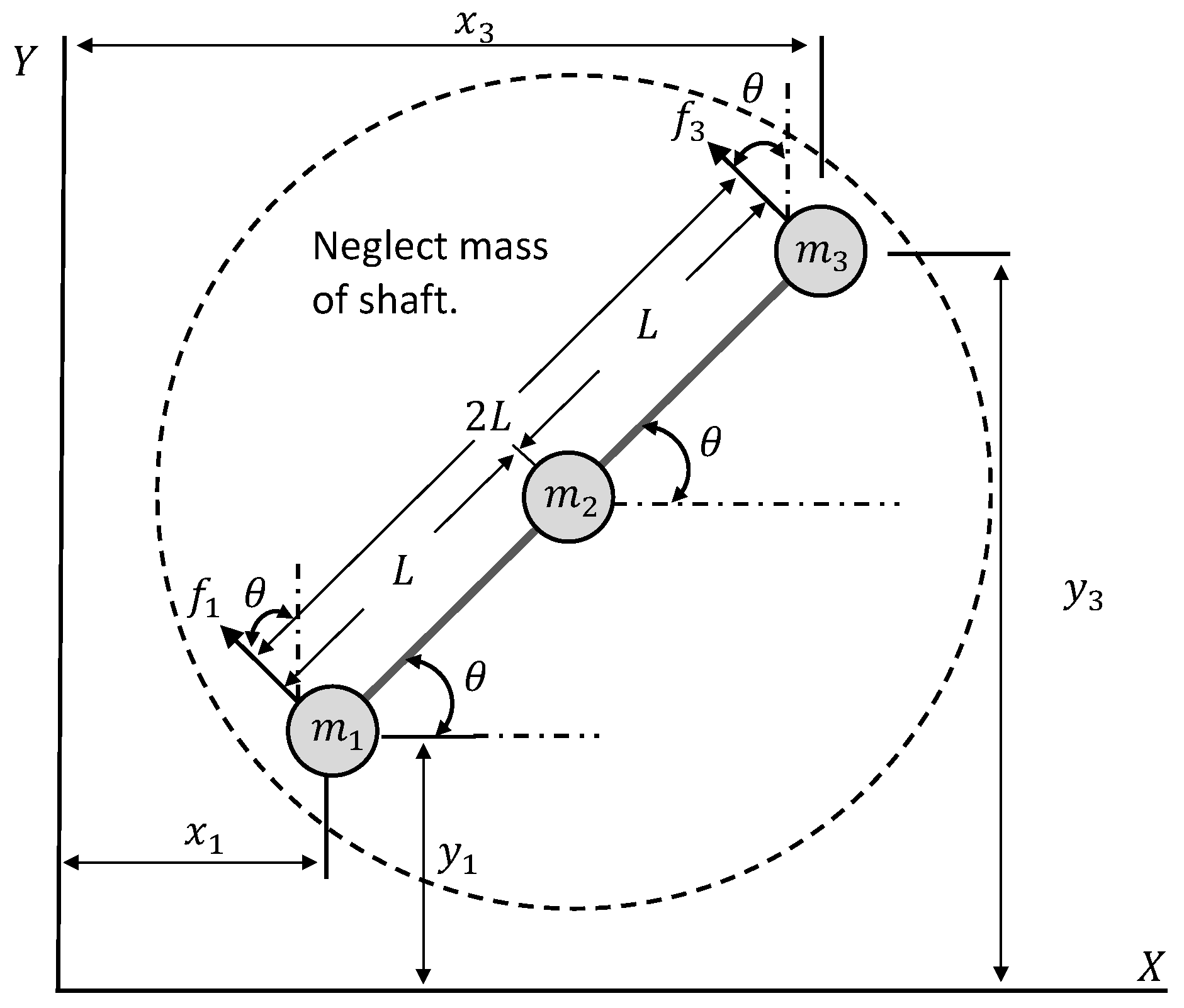
We consider an underactuated robot system with masses
,
, and
, as shown in
Figure 1 that are rigidly fastened to the mass-less shaft and are free to move in the 2D plane. We now set up the equation of motion of the holonomic robot using convenient coordinates
. An external force
is applied to
in the direction of
and
respectively, and
to
in the direction of
and
respectively. To simplify the notation, we assume that all representative particle masses are the same (e.g.,
for
). Applying Lagrange’s equations, it immediately follows that
where
is positioned at the center of the first mass particle,
L is the distance between each mass, and
is the inclination angle (see
Figure 1). The equations of motion can be written in compact form as
where
is the generalized inertia matrix
is the Coriolis matrix
with
Therefore, the elements of the inertia matrix for the holonomic robot are given by
The virtual work is given by
The derivation of (
32) is given in
Appendix A. Without loss of generality,
can be written as
with
. Therefore,
and
. Note that
is an invertible
matrix.
Mechanical Properties of the Underactuated Robot
The robot as defined by (
27) has several fundamental properties, which can be used to facilitate the design of an automatic control mechanism.
- P.1
is a positive definite matrix.
- P.2
The inertia matrix depends only on the actuated variables , i.e., .
- P.3
The sub-block matrix of the inertia matrix is constant.
- P.4
From (
28) and (
29), and by using (
30), we get
which is a skew-symmetric matrix.
The system has three degrees of freedom and only two actuators, hence, we have an underactuated mechanical system. We have nonlinearities because the generalized inertia matrix is off-diagonal and the input matrix is highly coupled. Due to the lack of more actuators, this system cannot be fully linearized using exact feedback linearization. However, it is still possible to apply PFL to the system, such that the translational dynamics and become a double integrator. As already mentioned, PFL compromises the robustness of the closed loop. However, the PFL can be avoided by using the proposed transformation, as shown in Corollary 1. Given the properties P.1–P.4, we apply the generalized coordinate transformations based on Proposition 1 to decouple the system.
Proposition 2. Considering the holonomic robot in (27), the dynamical system model can be rewritten as Proof. By applying Proposition 1 the result follows. □
In the next section, we address questions related to the automatic control of a particle swarm that minimizes energy by applying the transformed underactuated model in (
35)–(
37). We prove that the mean of configuration variables is controllable and provide conditions under which the variance is also controllable.
4. Control Design for a Swarm
In this section, we present an automatic controller for a swarm of particles that minimizes energy. We show that it only relies on the first two moments of the swarm configuration variables, i.e., the position and the orientation angle distribution. The main objective of our automatic control approach is to act on forces optimally so that particles can reach the desired target position with the stable Euler angle ().
4.1. Swarm Dynamical System Model
By defining
, the dynamics of (
35)–(
37) can be written as
The elements of
and
are
The system is nonlinear, since matrices
and
both depend on the current state variables. Firstly, we analyze the number of controllable states as given by the following definition.
Definition 1. The states in (38) are controllable if the pair is point-wise controllable. This can be observed by the rank of the controllability matrix The consequence of Definition 1 is that the
matrix for the system in (
38) has the full rank (i.e., rank
). Therefore, all states are controllable. Previous work has shown that the mean and variance of many particles for simple fully actuated particles are controllable [
5,
7]. Next, we show how we can stabilize the nonlinear underactuated particles by a global state-feedback controller designed via state-dependent Riccati equation (SDRE) control [
14]. Motivated by (
38) and defining the mean states
that represent the mean states of
N particles, we can write the dynamical system model of the swarm as
Interestingly, analyzing the controllability of the swarm dynamics results in the same form as in (
38), hence, the mean states are controllable.
4.2. Control Law
Our objective is to find minimum energy inputs that steer the swarm to a given target state defined on
. To do so, consider now the following cost functional
with respect to the state
and control input
u subject to the nonlinear dynamical system model constraint
where
penalizes the state, and
penalizes the control effort for all
. We aim for a nonlinear state-feedback controller
u that stabilizes solutions of problem (
41) and (
42).
Remark 3. Cloutier [14] obtains the nonlinear feedback controller via SDRE. Our interest is to provide an alternative interpretation of solving the problem (41) and (42) via Pontryagin’s minimum principle [13]. From (
41) and (
42), the Hamiltonian can be written as
where
is the adjoint vector. The necessary condition is derived by differentiating (
43) with respect to
u which yields
We obtain the nonlinear feedback controller
Now, we define
, where the matrix
can be obtained by solving the algebraic Riccati equation
By that we fulfill the second optimality condition
Therefore, as long as the two conditions in (
44) and (
47) hold, it is always possible to construct a nonlinear feedback controller that solves the problem (
41) and (
42). The closed-loop solution for this feedback controller is at least a local optimum and possibly the global optimum.
4.3. Stability Analysis
Theorem 1. Consider the dynamical system model (41), with the feedback controller (45). Assume in addition that for a constant input weighting matrix , the state weighting matrix can be chosen, such that for all x, where is the solution of (46). Then the zero equilibrium of the closed-loop system is semi-globally stable. Proof. Consider the Lyapunov function candidate
the time derivative of which, along the trajectories of the closed-loop dynamical system, is such that
where
. In addition, based on the assumed selection of
, yields
and
, hence our claim. □
4.4. Controlling Mean and Variance
The variances
and
of
N underactuated particle’s position is
The objective now is to control both, the mean and variance, effectively to ensure approaching a target position with minimum variance. Therefore, the selected strategy is the hysteresis-based approach following [
5,
19]. The idea is that the automatic controller regulates the mean states of
N underactuated particles with radius
r but switches to minimizing variance if the variance exceeds the threshold
and until
is reached [
5]. The idea of using such values comes from Graham and Sloane [
8]. They proved that the minimum variance to collect
N 2D circles with radius
r is
. Our proposed methodology in total consists of (1) applying the generalized coordinate transformation shown in Algorithm 1 and (2) proposing and analyzing the control mechanism to regulate the mean and variance of the swarm of underactuated particles shown in Algorithm 2.
| Algorithm 1 Generalised Coordinate Transformation for Underactuated Particle (27). |
begin procedure
Step 1: Partition the generalized coordinates and velocity w
Step 2: Construct the invertible mapping
with
Step 3: Apply Proposition 1.
end procedure |
| Algorithm 2 Hysteresis-based Mean and Variance Automatic Control |
Require: Knowledge of underactuated particle swarm mean , variance , the boundary of the search space , and the desired mean state .
,
loop
if then
∣
else
∣
end
if then
∣
else
∣
end
Apply the automatic control law (45) to regulate the underactuated swarm to the desired state
end loop |
4.5. Fully-Actuated vs. Underactuated Particle Swarm
We now consider a small swarm of
particles to showcase the performance of the proposed control law and highlight the advantage of the underactuated particle swarm over the fully-actuated swarm [
5]. The sampling time is set to
s and the physical parameters are given in
Table 1. The control gain matrices
and
are based on the assumptions of Theorem 1 and we get
We compare it to the approach of Shahrokhi et al. [
5]. Their control gains for the PD controller are
,
,
, and
.
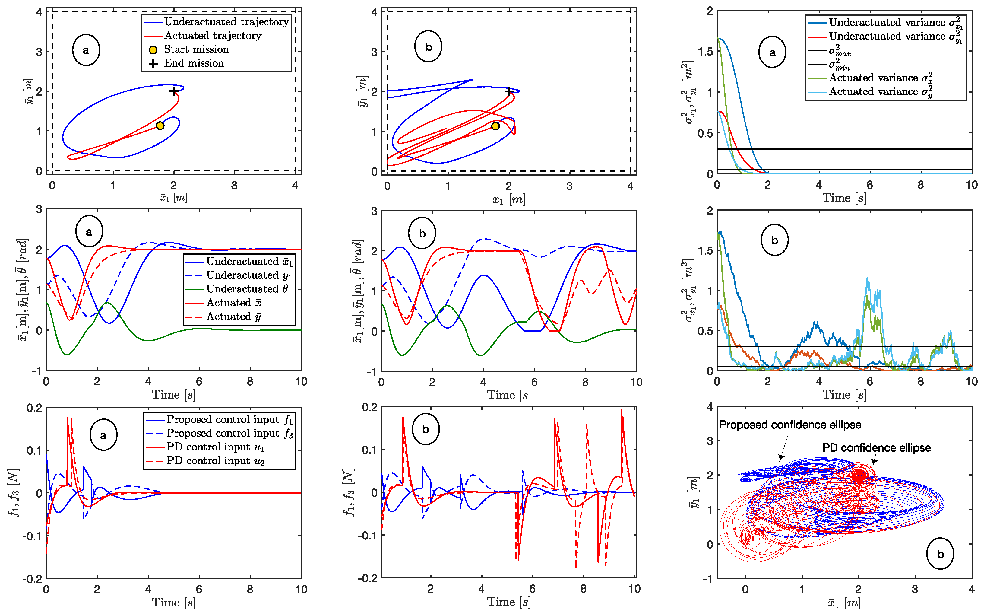
Figure 2 compares our approach and the PD controller [
5] for the obtained trajectories of mean, variance, and the control inputs. Even though the settling times seem satisfactory for both approaches, the trajectory and the control inputs allow us to discriminate between the two approaches. The control inputs obtained through our approach are significantly smaller resulting in less energy consumption. Also, note that there are no sudden peaks in the control inputs. The fully-actuated approach consumes
of energy compared to the under-actuated one that consumes
. This is an energy reduction of approximately
.
Both approaches minimize mean and variance. However, in the underactuated case, we stabilize the mean Euler angle with only two global control inputs. Hence, we reasonably balance the tradeoff between control complexity and system performance.
5. Multi-Robot Simulations and Discussion
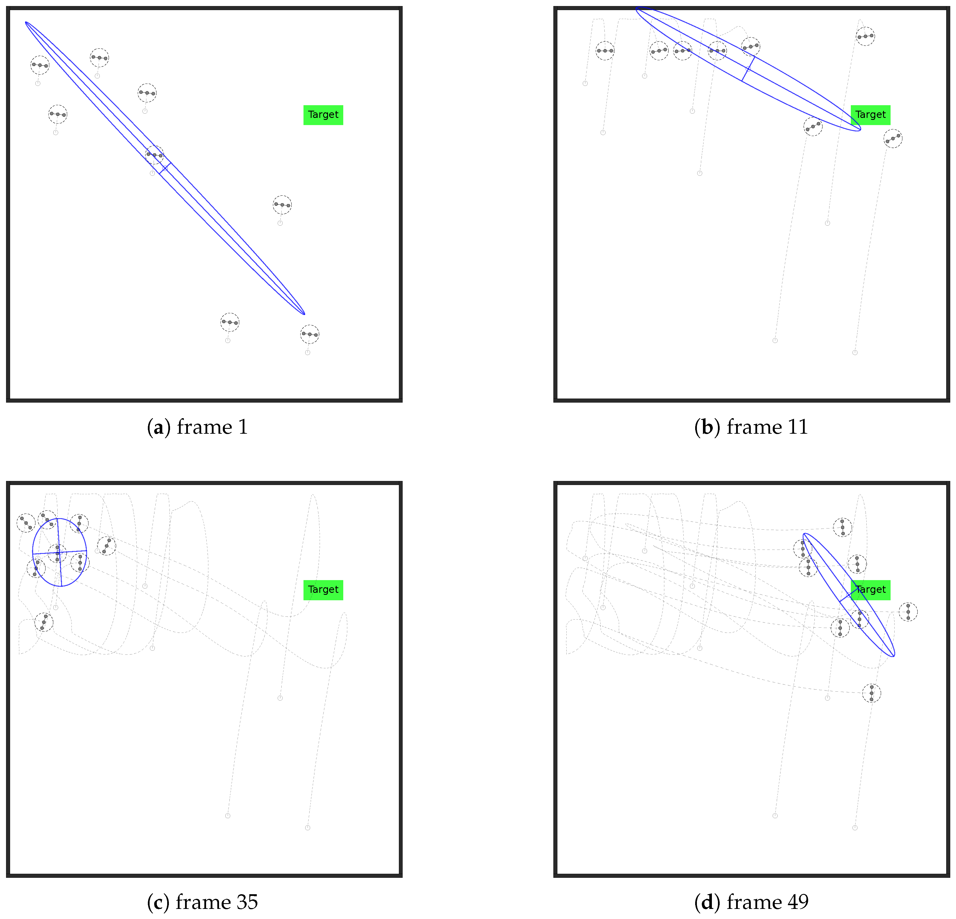
We also show the result for a swarm of
robots to visualize our results in an accessible way. Time is discretized and the control signal is scaled by
. The underactuated robots and arena boundaries are simulated as physical entities. Each underactuated robot has a random initial pose and the swarm’s mean position has a randomly generated target pose. The nonlinear controller described in Algorithm 2 steers the robot’s from a starting position to a target position (equilibrium point of the swarm) with a stable Euler angle.
Figure 3 shows four screenshots during a representative simulation run. This result shows how the properties of the underactuated robot system (e.g., torque and inertia) are exploited to regulate the mean, to minimize the variance, and to steer the swarm to the target on the right pose.
Looking ahead there will be a need for the further abstraction of details like actuators and engines, making it a building-blocks tool using various components. There are several limitations of the automatic control mechanism at this time. At this stage of the method development, non-holonomic constraints do not consider. Furthermore, we only tackle to track only the boundary of a ‘cloud of robots’ and their center of gravity. Possibly also the particle density could be measured instead of each individual robot.


