
Selection Rules for Resonant Longitudinal Injector-Coupling in Experimental Rocket Combustors

Institute of Aerodynamics and Flow Technology, Spacecraft Department, German Aerospace Center (DLR), Bunsenstrasse 10, 37073 Göttingen, Germany
Aerospace 2022, 9(11), 669; https://doi.org/10.3390/aerospace9110669
Submission received: 6 September 2022
/
Revised: 10 October 2022
/
Accepted: 12 October 2022
/
Published: 29 October 2022
(This article belongs to the Special Issue Liquid Rocket Engines)
Abstract
:This paper investigates different types of longitudinal mode coupling in subscale rocket combustion chambers using experimental data and numerical simulations. Based on a one-dimensional planar wave acoustic model of coupled cavity resonators with two acoustic inlet boundary conditions, mode selection rules are derived, providing a simple way of predicting which injector and combustion chamber modes have matching frequencies. Longitudinal mode coupling of an injector with an acoustically open inlet boundary condition has been reported in the literature for the start-up transient of a research combustor experiment. In this experiment, every third injector mode couples to a corresponding chamber longitudinal mode, which is explained in terms of the selection rules derived in this paper. Numerical simulation results for a different combustor experiment show an unexpected mode coupling behavior when an acoustically closed injector inlet is used. Theoretical analysis by using the one-dimensional wave model and applying the derived selection rules shows that in this setup, the injector acoustic mode can accommodate two different acoustic boundary conditions at the injector-chamber interface simultaneously. This results in different acoustic mode shapes in the injector, explaining the unexpected behavior for the resonant coupling with an acoustically closed injector inlet.
1. Introduction
Despite considerable development effort since the beginning of space exploration in the 1950s, combustion instabilities in rocket thrust chambers are still not fully understood and remain one of the main concerns in the development of new engines. Combustion instabilities are strong acoustic disturbances that can damage or destroy rocket engines within short periods of time. Among other types of instabilities in flight-scale rocket engines, high-frequency transverse oscillations have been identified as the most dangerous ones and were investigated in numerous studies, see e.g., [1,2]. Apart from space propulsion applications, dangerous combustion instabilities are also found in other types of combustion systems like aircraft engines, boilers and gas turbines. A systematic overview for transverse combustion instabilities in air-breathing systems has been compiled by O’Connor et al. [3]. Different physical mechanisms and their mutual interaction determine the stability behavior of combustion devices. However, so far, no conclusive explanation has been given which processes eventually lead to the onset of combustion instabilities. Experimental studies in the past indicated a strong effect of the hydrogen temperature on the stability margins [4] of a rocket combustor. A recent study [5] assessed the role of hydrodynamic effects, e.g., vortex shedding, behind shear coaxial injectors that may also lead to a modulation of the heat release rate in the combustion chamber. Another possible instability mechanism that has been observed in rocket combustion chambers [6], as well as air-breathing combustion systems (cf. Section 3.2.1 of [3]), is injector-coupling. Injector-coupling refers to the acoustic coupling of pressure waves in the injector and the combustion chamber and has been observed experimentally in different combustion chambers and for several fuel oxidizer combinations [7,8,9]. Experiments in subscale rocket combustors [6,10] suggest that resonant coupling between the oxygen injector and chamber eigenmodes might be a necessary condition for the occurrence of combustion instabilities. Most of the published work on injector-coupling and combustion instabilities investigates coupling between oxygen-injector longitudinal and transverse combustion chamber modes (see e.g., [6]), as transverse modes are typically the most unstable modes for flight-scale and subscale multi-injector rocket engines. However, experimental studies of single-injector configurations [11,12] showed that also coupling of longitudinal modes can be observed. The study of Klein et al. [12] reported longitudinal injector-coupled combustion instabilities for the first time during ignition testing in a liquid oxygen (LOx)/methane subscale combustor. A detailed analysis showed that mode coupling between the third injector longitudinal eigenmode with the first longitudinal chamber mode occurs, but also that this coupling extends to higher injector and chamber modes. This behavior has not been observed before with longitudinal-transverse coupling, and it remains unclear if higher mode coupling contributes to the observed combustion instability.
Longitudinal injector-coupling has also been investigated experimentally and numerically in the European Space Agency (ESA) Technology Development Element Program “Visualizing injector-coupled combustion instability in LOx-H flames”. Numerical simulations of mode coupling for a single injector subscale rocket combustor showed a very similar coupling pattern compared to the experimental results in [12]. However, unexpected coupling of higher modes was observed in these simulations, which needed further analysis.
The purpose of this paper is therefore to present a theoretical model for different resonant longitudinal coupling scenarios and to derive a set of selection rules to identify modes with identical frequencies.
Depending on the acoustic boundary condition at the inlet of the injector, the theoretical model for longitudinal mode coupling predicts different possible coupling scenarios. This paper will investigate injector-coupling for an acoustically open injector, as well as an acoustically closed injector inlet. An acoustically open injector can be assumed, for example, if the injector pipe is connected to a manifold with a large volume that distributes the oxidizer to the various injectors. This situation corresponds to the experiment of Klein et al. [12], to which the theoretical model is successfully applied to. An example of an acoustically closed injector inlet has been encountered in numerical simulations of the single-injector experiment from the ESA project “Visualizing injector-coupled combustion instability in LOx-H flames”. For this setup, the coupling model not only explains the observed mode coupling scheme, but also predicts the surprising coupling of unexpected additional acoustic modes.
2. Acoustic Analysis of an Injector-Combustion-Chamber System
The acoustic analysis of the injector-combustion-chamber-system follows closely the analysis and the notation of Schuller et al. [13]. Their work intended to deliberately decouple three acoustic cavities while in this work, I will investigate the resonant coupling between two cavities.
The acoustic setup consists of a simplified single-injector combustion chamber of length and diameter , and an injector pipe of smaller diameter and length connected to the chamber volume, see Figure 1. In this setup, it is assumed that the thermodynamic gas properties in the injector and the combustion chamber are constant, and that an infinitely thin flame is located at the injection location . The properties of the fresh unburnt gas in the injector are labeled by the subscript u while the burnt gas properties are denoted by the subscript b.
This work considers only longitudinal acoustic waves with amplitudes in the injector region (denoted by 0) and the chamber region (denoted by 1) of the setup, see Equations (1)–(4). In these expressions, the wave number k is given by where f and are the oscillation frequency and the angular frequency, respectively.
The acoustic waves in the two regions are complemented by the jump conditions at location that enforce continuity of the pressure at the flame location (Equation (5)) and a jump in acoustic velocity due to the heat release in the flame (Equation ()).
The jump condition for acoustic velocity Equation (6) also contains the ratio of specific heats of the burnt gas, as well as the cross sectional areas of the injector and the combustion chamber .
Self-sustained oscillations can develop if the heat release rate depends on the acoustic variables [13,14]. Such a model, also known as the flame transfer function, allows to identify the most unstable modes of the coupled system by means of stability analysis. However, any interaction between the heat release rate and the acoustic waves will be neglected in this work as only the coupling of acoustic waves without flame amplification shall be investigated. Previous studies [15] showed that this assumption is justified for uncoupled systems because the frequencies of the unstable modes are located in the vicinity of the unexcited system eigenfrequencies.
Boundary conditions at the inlets and outlets constrain possible acoustic modes. At the nozzle outlet of the chamber, a solid wall is assumed following the discussion in Marble et al. [16] who showed that this is the limiting case for small approach Mach numbers in the burnt gas region. Therefore,
At the injector inlet position , two different boundary conditions are investigated:
In this work, I will consider an acoustically open injector (Equation (8)), as well as an acoustically closed injector (Equation (9)). Typically, the assumption of an acoustically open injector is reasonable for an experimental combustion chamber setup because the injector is connected to a manifold. On the other hand, numerical inflow boundary conditions at subsonic speeds often behave like acoustically closed ends [17] and therefore require some adjustments to adapt the numerical model to the experimental setup.
Applying the boundary and jump conditions Equations (5)–(9) to the planar acoustic waves Equations (1)–(4) results in a set of equations that can be written in matrix form
where X denotes the vector of unknown wave amplitudes,
Y is a given source term vector with
and M denotes a matrix that contains the continuity and jump conditions of the waves. Depending on the acoustic type of the injector inlet, two different matrices are formed. For the acoustically open inlet, the matrix M is written as
For an acoustically closed injector, the first row of the matrix is changed and M is given as
These matrices contain the acoustic coupling index given by
with S being again the cross-sectional area of the injector or the combustion chamber. The acoustic coupling index measures the coupling between elements upstream and downstream of the compact flame [13] and is of the order of for the single-injector combustion chamber which will be introduced in Section 4.2.
The eigenmodes of the system are given by the roots of the dispersion relation which is found by solving for . For the open injector, one finds the dispersion relation
For the closed injector, the dispersion relation only has imaginary values as indicated by the imaginary unit i, and takes the form
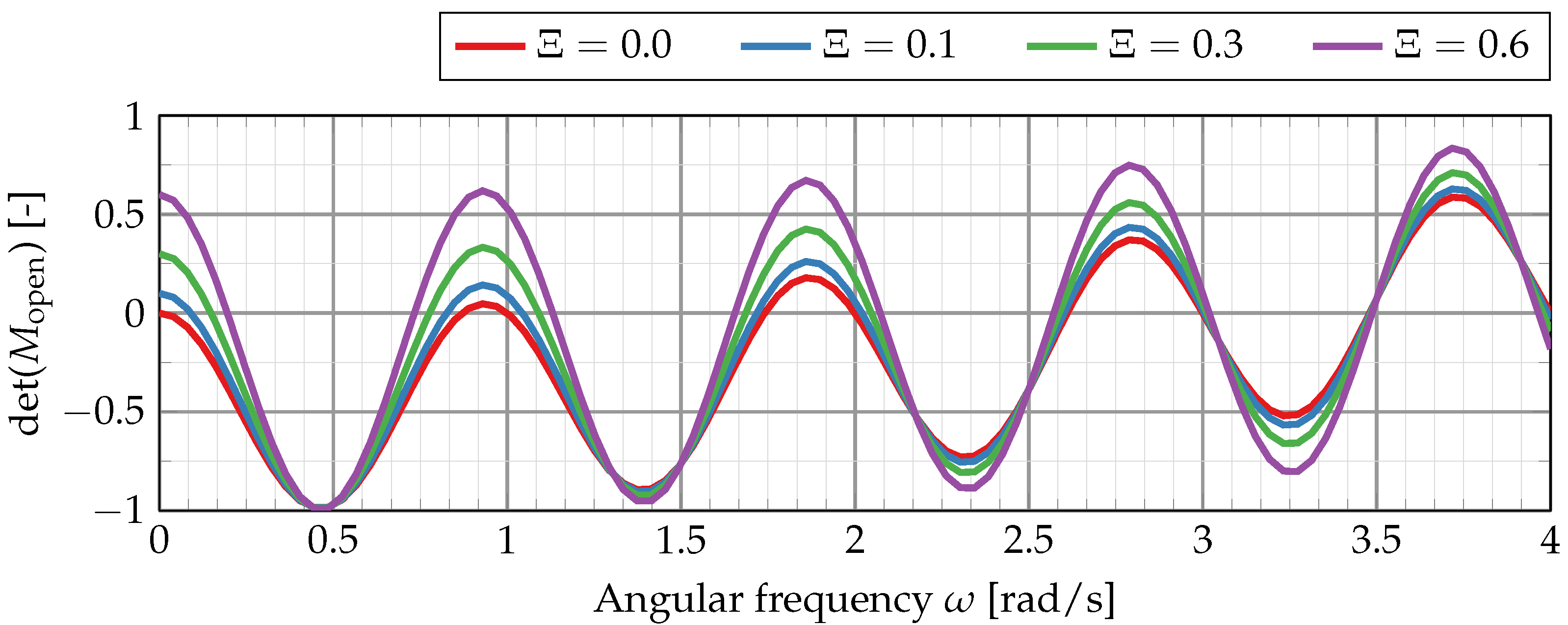
The value of the dispersion relation for different oscillation frequencies of a generic injector-chamber configuration is shown in Figure 2.
This first example shows the periodic spacing of the system eigenmodes, which are the roots of the dispersion relation det . Here, injector and chamber eigenmodes appear in pairs with varying frequency spacing. One notices the roots at s etc. which are the chamber eigenmodes. Injector modes are multiples of the fundamental frequency of s. The spacing between the separate eigenmodes is also influenced by the acoustic coupling index which increases the frequency spacing for the first eigenmodes for values .
Using the assumptions of plane waves (Equations (1)–(4)) together with the boundary and jump conditions Equations (5) and (6) allows to obtain the unknown wave amplitudes X. For the open injector, one finds
For a closed injector, the amplitudes are slightly different due to the different acoustic type at the inlet:
These expressions will be used later to investigate the acoustic mode shapes and to associate them with fundamental pipe modes.
3. Derivation of Mode Selection Rules for Resonant Coupling
In this section, I will derive a set of simple selection rules describing mode coupling between the injector and the chamber under resonant conditions. Resonant coupling occurs when any eigenfrequency of the injector is identical to another mode eigenfrequency of the chamber. For simplicity, it will be assumed that the frequencies of the first longitudinal injector mode (1L) and combustion chamber mode (1L) are identical and that these modes are therefore coupled. Such specific coupling of modes will be denoted by the shorthand notation 1L↔ 1L throughout the remainder of this paper.
I will also assume a vanishing acoustic coupling index throughout most of the paper. The reason behind this simplification is to first examine the idealized case of the independent injector and combustion chamber modes, and later extend the model for small coupling indices as they can be found in typical setups for injector-coupling. The analysis will be conducted for an open injector as well as a closed injector type.
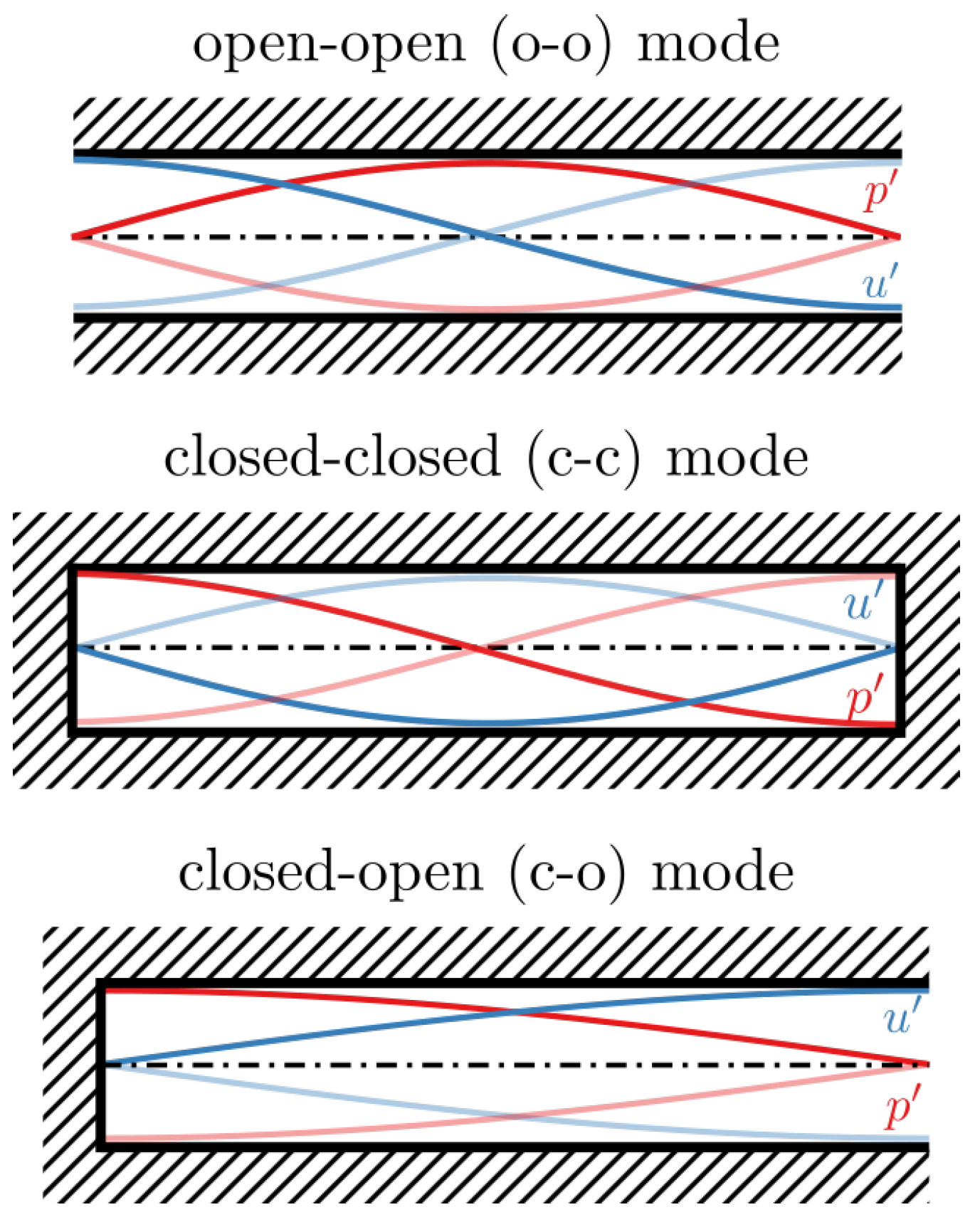
The purpose of this section is to express the acoustic modes of the injector and the combustion chamber in terms of the fundamental pipe mode shapes shown in Figure 3.
Based on these pipe modes and the type of acoustic boundary condition at the injector inlet, different coupling scenarios between the chamber and injector are possible. For the acoustic mode shapes in Figure 3, one can relate the mode frequency to the mode index n, the cavity length L and the speed of sound c by
3.1. Resonant Mode Coupling with an Open Injector
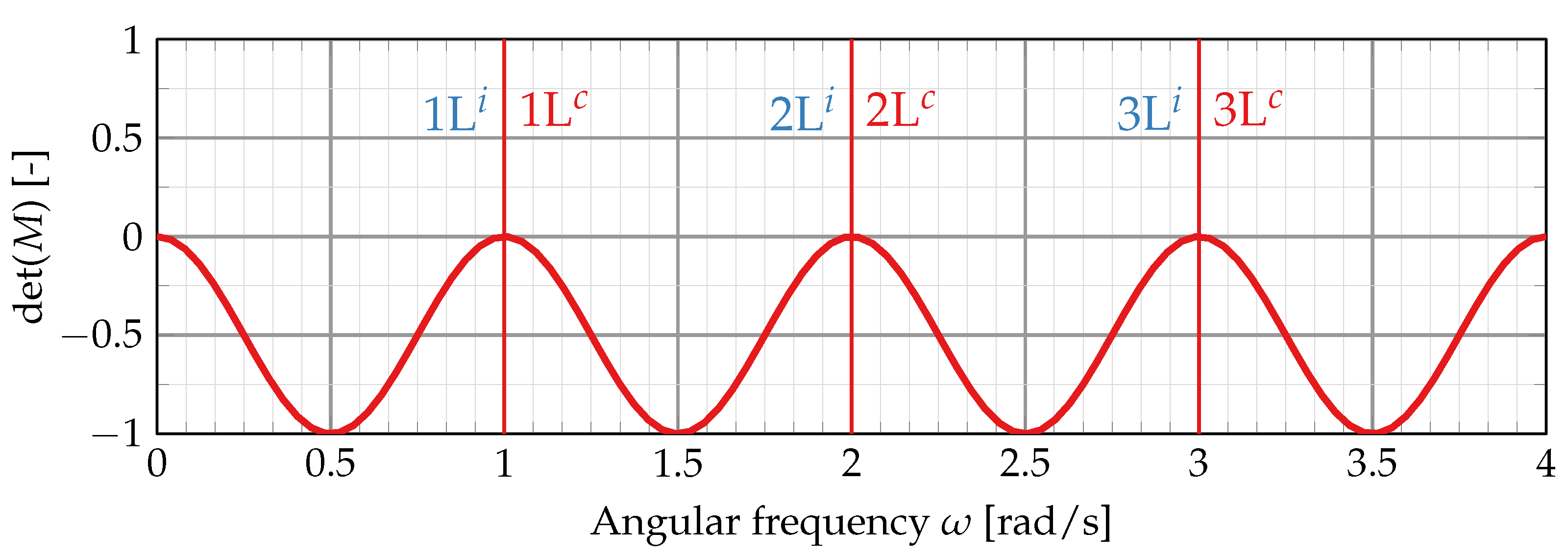
The first case considered here is acoustic mode coupling with an open injector. Both the injector and the chamber have their fundamental 1L frequency at s. This results in a dispersion relation that shows coinciding eigenfrequencies for injector and chamber evenly spaced at integer values of the angular frequency, see Figure 4.
For ideal resonant coupling with an open injector, not only the first longitudinal modes couple but also higher ones, e.g., 2L↔ 2L, 3L↔ 3L, etc. This can be understood if one assumes that the coupled systems consist of an acoustically fully closed combustion chamber, to which a fully open injector is attached. It is reasonable to assume that the combustion chamber is of closed-closed type (see Figure 3) because of its convergent-divergent nozzle (cf. also the discussion in [16]) and the solid wall injection plane at the chamber entrance. For small or vanishing acoustic coupling indices, one can assume that most of the injection plane consists of a solid wall and only a small area connects the chamber to the injector. Therefore, the assumption of a closed-closed combustion chamber is satisfied.
However, the acoustic type of the injector is not immediately apparent because of the constant cross-section and its connection to the larger combustion chamber volume. As a first guess, the assumption of an open-open injector seems reasonable because of its common interface with the much larger combustion chamber volume, similar to a pipe discharging into the atmosphere. On the other hand, the combustion chamber pressure will oscillate and therefore could also act on the injector pressure wave as a virtual solid wall. Gröning et al. [6] discuss the acoustic configuration of the injector and conclude that an open-open configuration is the most likely one. It will be shown later that both injector configurations (open-open and open-closed) can coexist at the same time, depending on the initial choice of coupled modes.
Assuming that the injector is of open-open type (Equation (27)) and the chamber is of closed-closed type (Equation (28)), resonant coupling of the injector mode with the first chamber eigenmode (mode 1L ) occurs:
This equation is used to express the injector frequency Equation (27) in terms of combustion chamber quantities:
Equating the right hand side of the equation with the closed-closed frequency Equation (28) of the chamber gives the selection rule for type-1 mode coupling:
For , there is a trivial one-to-one mode coupling between injector and combustion chamber, i.e., 1L 1L, 2L 2L, etc. This corresponds to the eigenmodes given by the dispersion relation shown in Figure 4.
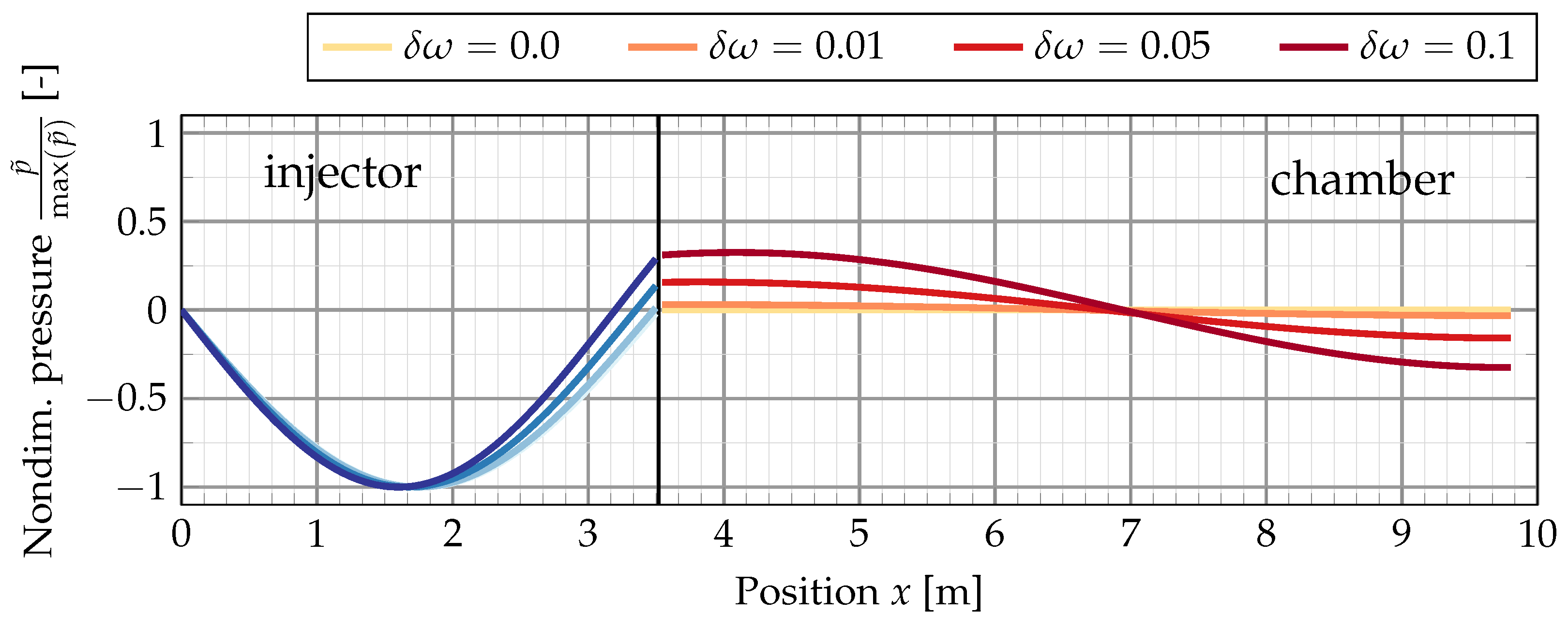
Figure 5 shows the normalized pressure mode shapes in the injector and the chamber for different oscillation frequencies that approach the resonance frequency s.
One notices that the ratio of the injector-to-chamber amplitude goes to infinity as the frequency approaches the resonance frequency:
This behavior only applies to the idealized case with . For there is a small frequency shift between the injector and chamber eigenfrequency which leads to a finite even for . It is important to note that the injector amplitude will be much larger than the chamber amplitude in the resonant case, and not vice versa. The mode shapes in the injector and the chamber also agree with the initial assumption of an open-open injector connected to a closed-closed combustion chamber in the resonance limit.
3.2. Resonant Mode Coupling with a Closed Injector
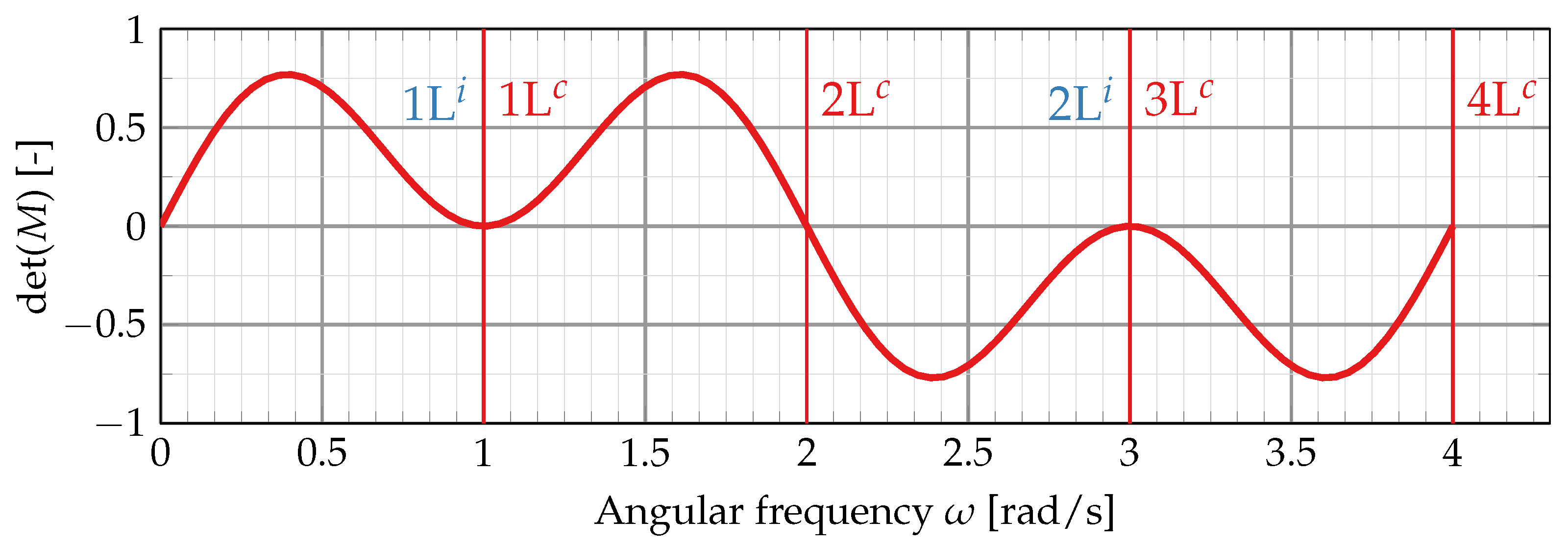
Resonant mode coupling between a closed injector and a closed-closed combustion chamber shows a slightly different behavior, as indicated by the dispersion relation in Figure 6.
One can now apply a similar analysis as before assuming that the injector’s fundamental mode shape corresponds to a closed-open pipe mode whose frequency is given by Equation (29). For the combustion chamber, it is once again assume that it is acoustically closed on both ends.
As before, the frequency of the -th injector mode is matched with the first fundamental mode of the chamber and selection rules are derived from this.
I again express the injector frequency in terms of the chamber quantities
and compare this to the equation of the closed-closed chamber frequency Equation (28) to obtain the selection rule:
This equation has solutions for certain combinations of and allowing for mode coupling in this setup. For , one finds a coupling between the modes 1L 1L, 2L 3L, etc. Note that this type of coupling only involves odd-numbered chamber modes and corresponds to the case depicted by the dispersion relation in Figure 6.
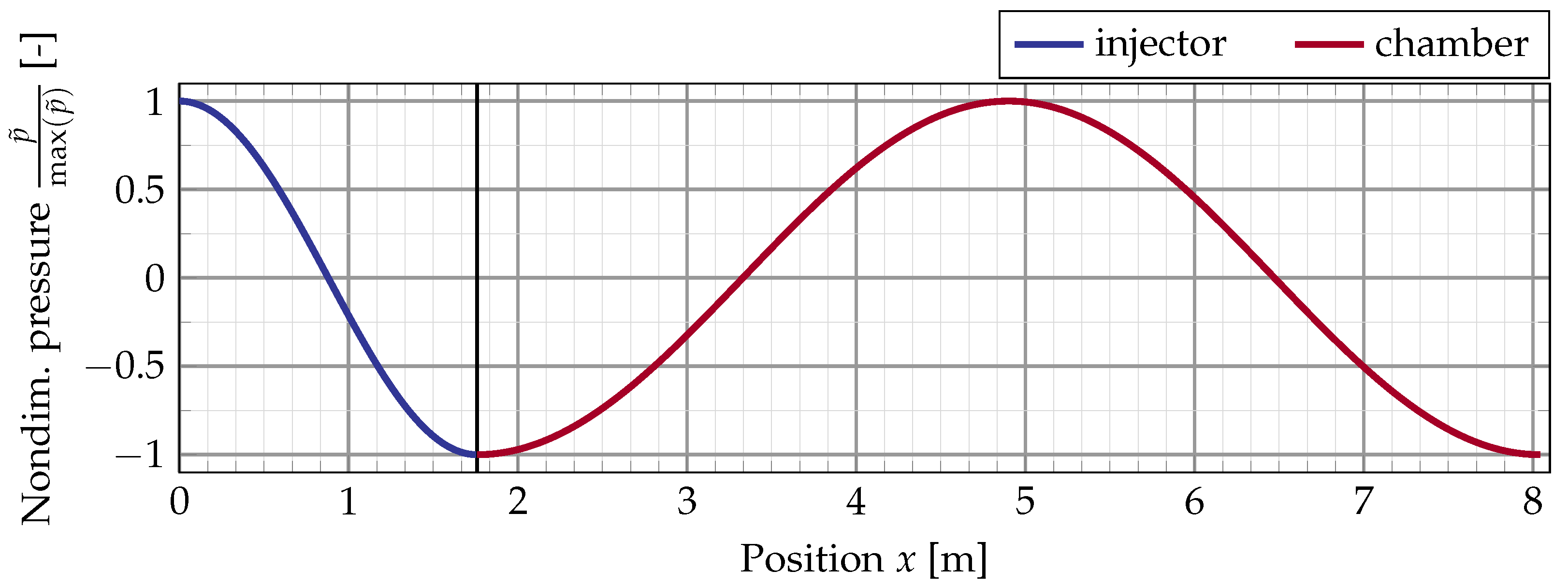
The dispersion relation, however, shows additional resonant chamber modes at integer multiples of s that do not have any corresponding closed-open injector modes. In order to investigate these modes, Figure 7 shows the pressure mode shapes in the injector and chamber for this eigenfrequency.
In contrast to the intended coupling between a closed-open mode of the injector with a closed-closed chamber mode, the eigenmode at s is a closed-closed injector mode coupled to the 2L chamber mode. It is also interesting to note that for this type of coupling, none of the modes dominate and that the injector and chamber amplitudes are equal. This idealized acoustic configuration, therefore, shows that in contrast to the previous initial guess in [6], a coupled resonant injection tube can accommodate different acoustic modes at the same time.
This behavior of the closed-open injector to closed-closed chamber coupling type is further analyzed in terms of the simplified mode selection rule method.
For this, I express the closed-closed injector frequency in terms of closed-closed combustion chamber modes by replacing by Equation (34)
and compare this to the frequency for the closed-closed injector. This gives the selection rule for an additional closed-closed to closed-closed coupling even though the initial frequency matching was based on a closed-open injector and a closed-closed combustion chamber setup:
Selection rule Equation (38) can be fulfilled showing that there can be a simultaneous coupling of different acoustic configurations if the initial frequency matching is based on the fundamental chamber mode and the th injector mode. For , one finds the mode coupling 1L 2L, 2L 4L, etc. which is complementary to the previous selection rule as it involves the even-numbered chamber modes.
4. Results
In this section, the results from the previous theoretical considerations will be used to explain different mode coupling scenarios found in an experimental study using an open injector and a numerical investigation with a closed injector.
4.1. Open Injector Coupling during Ignition Testing of a Subscale LOx-Methane Rocket Thrust Chamber
An example of mode coupling with an open injector has been observed experimentally [12] during start-up of the experimental LOx-methane rocket combustor A (BKA) at DLR Lampoldshausen. BKA is a cylindrical combustion chamber with an inner diameter of 50 mm and an injector head consisting of 15 shear coaxial injection elements. The injector is connected to a LOx manifold and can therefore be considered as an acoustically open injector at its inlet. During the test runs, BKA is operated at subcritical chamber pressures up to about 9 bar. Klein et al. [12] report three different examples of start-up sequences of which two show severe combustion instabilities (Cases B and C). As the analysis did not reveal any apparent pattern of how the combination of inflow properties affects the stability behavior of the chamber, they investigated injector-coupling as a possible mechanism for combustion instabilities.
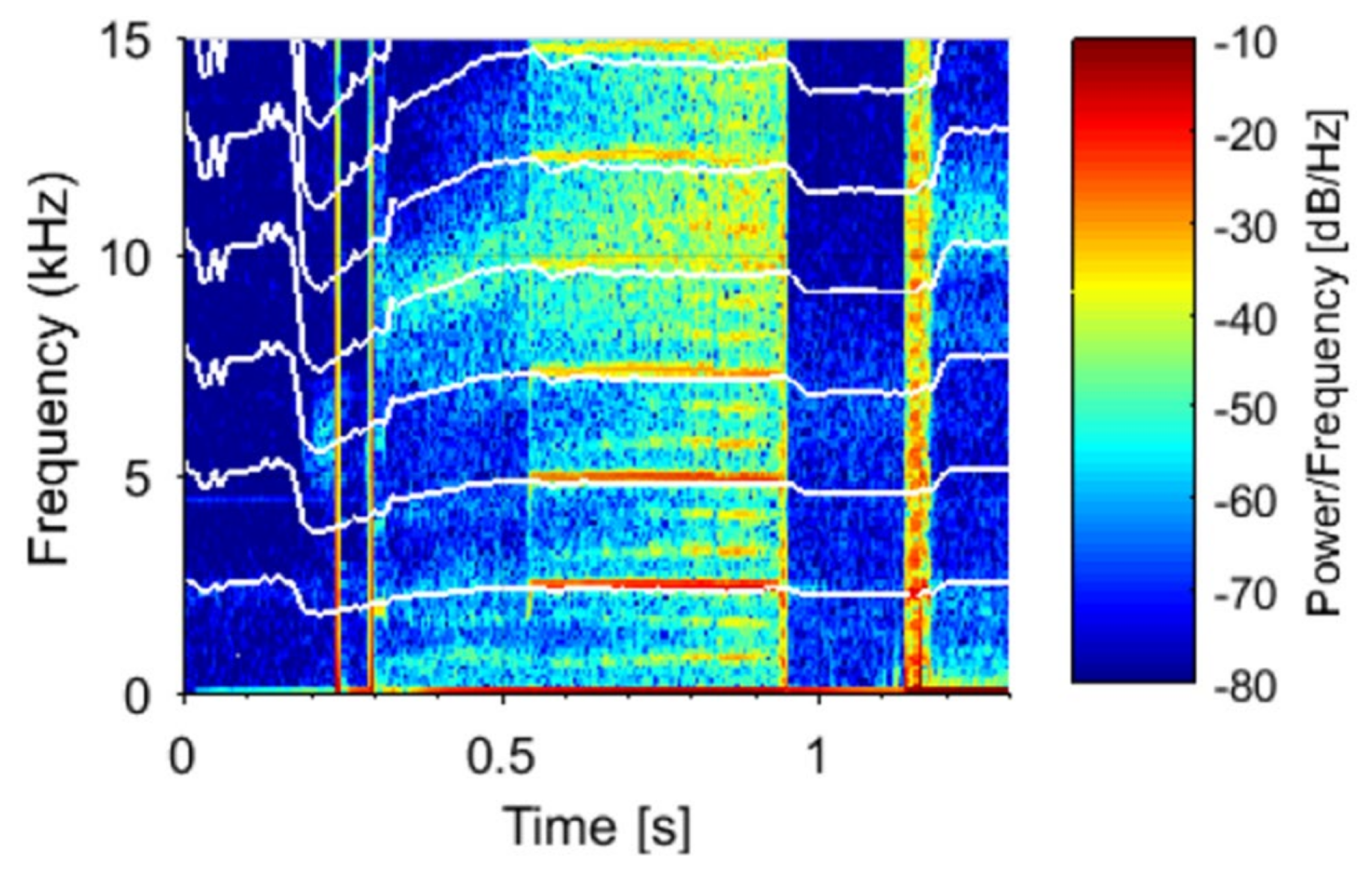
The experimental spectrogram Figure 8 compares the measured chamber eigenfrequencies (horizontal bands of high pressure amplitude) with the results for calculated chamber eigenfrequencies (white lines). These frequencies have been calculated under the assumption of closed-closed combustion chamber modes (cf. Figure 3) and a simplified hot-gas model for the thermo-chemical properties of the burnt gas.
The temporal evolution predicted by the simplified hot-gas model of Klein et al. [12] closely reproduces the eigenfrequencies in the transient start-up phase and successfully predicts the plateau of constant chamber modes during the phase of strong instabilities between and 1 s.
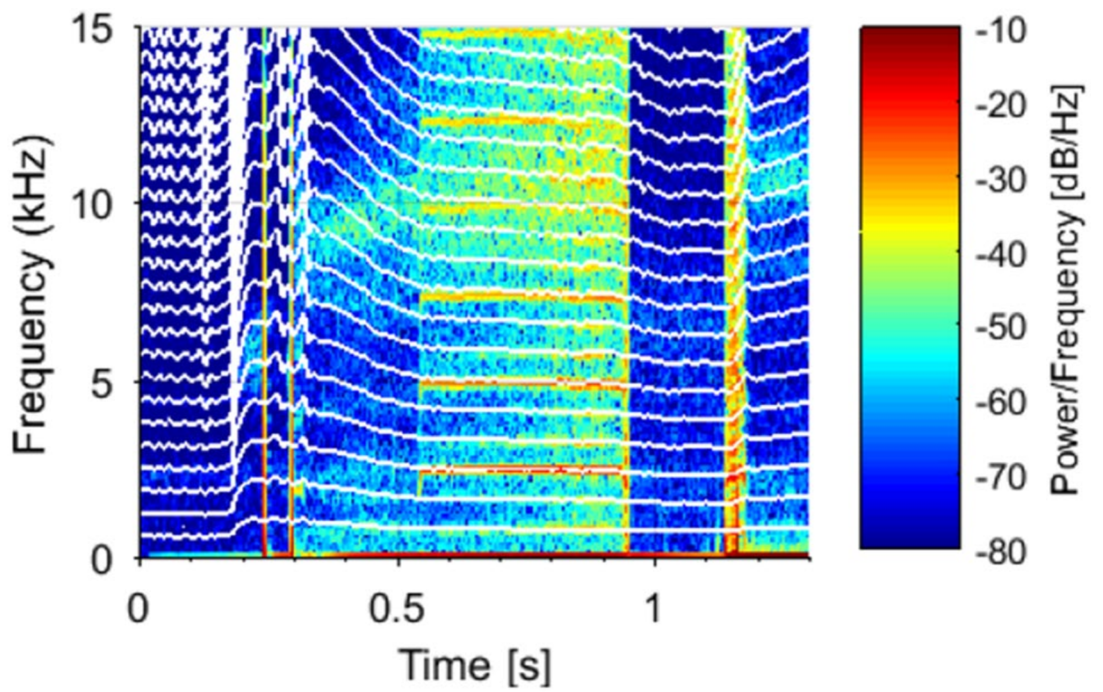
For acoustical properties of the injector, Klein et al. [12] developed a model for the speed of sound of the two-phase flow inside the oxygen injector. This model also accounts for strong pressure oscillations during the start-up sequence. Together with the assumption of an open-open cavity for the injector (cf. Figure 3), they calculated the temporal evolution of the LOx post frequencies shown in Figure 9 as white lines.
One notices the close matching of every third oxygen injector mode with the combustion chamber eigenmodes showing that injector-coupling occurred during this experiment. Based on this observation, the acoustic configuration of the chamber mode (closed-closed) and the injector (open-open) mode, it is concluded here that this experiment exhibits the mode coupling behavior outlined in Section 3.1 with (i.e., 3L 1L, 6L 2L, etc.).
4.2. Closed Injector Coupling in Numerical Simulations of a Subscale H/O Rocket Thrust Chamber
An example of a closed injector coupling is presented for a numerical study of the single injector combustion chamber N (BKN) [9,18] from DLR Lampoldshausen. BKN is a single-injector combustion chamber with a circular cross section that is operated in the range of 40 to 80 bar with sub- and supercritical oxygen. The choice of modeling the oxygen injector with an acoustically closed inlet has been motivated by the fact that in the experiment, the injector is separated from the manifold by an orifice to acoustically decouple the injector from the upstream piping system. This reduction in cross section with a subsequent increase of the flow speed suggests the use of an acoustically closed inlet. Apart from that, the numerical inflow boundary condition in the flow solver prescribes a constant mass flow rate without restricting any pressure fluctuations in the field. Such a boundary condition describes an acoustically closed inlet. A more detailed explanation of the numerical boundary condition can be found in the numerical flow solver description below.
A summary of the BKN operating conditions is given in Table 1.
As no self-excited combustion instabilities were found in the BKN experiments and the accompanying numerical studies, a dedicated numerical test case with a forced harmonic excitation of the oxygen mass flux is used. The numerical study uses the second-order compressible finite-volume flow solver TAU developed by the German Aerospace Center DLR [19]. TAU uses an edge-based dual-cell approach on structured, fully unstructured and hybrid meshes. BKN is discretized as a half-model with 3.98 million grid points forming a hybrid mesh that consists of hexaeder, tetraeder, prisms and pyramids. Most cylindrical parts of the combustion chamber surface are discretized by quadrilateral elements. For a more flexible connection of small surface panels and in the connecting manifolds for window cooling and the H injector, surface regions are discretized using triangular elements. Inside the combustion chamber, the wall normal spacing of the first cell is chosen such that a nondimensional spacing of is realized. Because only half of the domain is used in the numerical simulations, a symmetry boundary condition is placed in the center of the combustion chamber. The mesh includes the full combustion chamber, the oxygen injector, the annular hydrogen injection including parts of the manifold, and the window cooling injection system (cf. Figure 10). Grid independence has been verified by increasing the mesh resolution in the front part of the combustion chamber near the face plate until the combustion chamber pressure, the wall temperature distribution and the flame shape did not change anymore in a steady Reynolds-averaged Navier–Stokes (RANS) simulation. This mesh has then been used for the unsteady simulations presented in this work.
Time-accurate simulations are performed using a Jameson-type dual-time stepping scheme [20] at a physical time step size of s. Numerical fluxes are calculated using the low-Mach-number [21] corrected version of the MAPS+ upwind solver [22]. Turbulent quantities of the flow are calculated using the Spalart–Allmaras model (referred to as the “standard Spalart–Allmaras model” on the NASA turbulence modeling resource website [23]) operated in unsteady RANS (URANS) mode. Chemical reactions are included by using the 6 species 7 reaction detailed chemistry scheme of Gaffney [24]. TAU solves additional equations for all participating species (H, H, O, O, OH and HO) and the chemical source terms are calculated using a modified Arrhenius approach. Due to the high pressure inside the chamber leading to near-equilibrium chemical reactions, the interaction between turbulence and chemical reactions is neglected. The real gas properties of O and H are considered by the Soave-Redlich-Kwong cubic equation-of-state [25]. All other species are included with their ideal gas properties. Viscous fluxes use a turbulent Schmidt number of 0.7 and a ratio of laminar-to-turbulent Prandtl number of 0.8.
All solid walls are modeled by an adiabatic viscous-wall boundary condition while the outflow boundary condition at the nozzle exit uses an exit-pressure outflow boundary condition. Special care is taken for the inflow boundary condition at the oxygen injector. This work uses a mass-flux boundary condition with fixed mass flux density ( = const.) and static temperature . As this (subsonic) boundary condition fixes the velocity fluctuations at the inlet and extrapolates the pressure from the inside of the flow field (i.e., the pressure at the inflow can oscillate freely), it is acoustically equivalent to a closed inlet. A more detailed investigation of the acoustic types of the boundary conditions in TAU and the general acoustic properties of the solver is given by Horchler et al. [17]. The acoustic properties of the inflow boundary towards the oxygen injector pipe are simplified here compared to the experiment. Using an acoustically well-defined boundary condition in the simulation, however, allows for much better control of oxygen mode frequency compared to the more complex situation in the experiment.
The numerical results are obtained in the following way: As a first validation step, a steady-state RANS solution for BKN is produced to compare the mean chamber pressure to the experimental results. As shown in Figure 11, the results are well within the experimental error bars, except for the last measurement location.
Then, in a second step, a strong pressure perturbation is added to the steady-state field and the simulation is continued using the time-accurate time stepping scheme (a more detailed discussion of the method can be found in [26]). By recording the decay of the pressure perturbation over time, one can find the chamber eigenmode frequencies in the pressure spectrum. Analyzing the wall surface pressure field using Dynamic Mode Decomposition (DMD) (see. e.g., [27,28]) also yields the spatial mode shapes, their frequencies and damping rates.
After the numerical chamber eigenmode frequencies are determined, one can simulate the injector mode coupling in BKN. In order to match the frequency of the injector to the first longitudinal chamber mode 1L, the length of the oxygen injector is modified as the speed of sound is fixed by the inlet temperature. As the acoustic configuration at the injector inflow boundary corresponds to a closed inlet and the injector opens out into the larger main chamber on the other end, a closed-open boundary condition (cf. Figure 3) is assumed for this setup. Together with the closed-closed acoustic mode of the chamber, this setup corresponds to the closed-injector configuration analyzed in Section 3.2.
The coupled simulation is then restarted from the steady-state solution with an oscillating oxygen mass flow at the inlet of to excite the injector and combustion chamber eigenmodes.
Figure 12 shows the combustion chamber pressure signal over the course of the simulation. Starting the simulation from a steady-state, a limit-cycle oscillation is reached after about 5 ms. Before that, the mean pressure drifts and the oscillation amplitude increases with time.
The chamber peak-to-peak pressure amplitude during the limit cycle is about 1 bar, which is much lower than the oscillation amplitude in the injector shown in Figure 13. Initially, the maximum pressure amplitude in the injector starts from 30 bar peak-to-peak and reaches up to = 40 bar.
Figure 14 compares the power spectral density in the limit cycle for the chamber and the injector pressure. Besides the apparent difference in pressure amplitude, both spectra agree in the position of their main peaks at 2579 Hz, 5159 Hz and 7738 Hz.
These frequencies represent the first three closed-closed combustion chamber eigenmodes that have been obtained from the impulse-response simulation. As this is an example of a closed-injector coupling with a matching of the first longitudinal injector mode with the first chamber closed-closed mode, selection rule Equation (36) with applies, giving
According to this rule, only the modes 1L 1L, 2L 3L etc. are coupled. However, this clearly contradicts the coupling at the 2L closed-closed chamber frequency which is not covered by the selection rule. This mode coupling can, however, be understood by the additional, simultaneous coupling of the closed-closed injector mode which is permitted in this coupling type. Here, the additional selection rule with applies, giving
Therefore, the first closed-closed mode of the injector couples to the second longitudinal mode of the chamber, which is observed in the spectrum. Additionally, coupling of higher modes 1L 2L, 2L 4L etc. is also possible.
In order to verify that the presumed mode coupling occurs in the test case, the spatial pressure mode shapes during limit-cycle oscillation are determined by DMD and are shown in Figure 15 for the chamber and Figure 16 for the injector. The figures show the spatial distribution of the pressure eigenmode , normalized by the maximum value encountered in the computational domain .
The analysis of the chamber mode shapes clearly confirms the assumption of a closed-closed mode in the combustor. All nodal lines are visible although the first mode is contaminated by noise near the injection plane.
Figure 16 shows the DMD results for the injector pressure field which confirms the assumption of a closed-open mode for the 1L and 2L modes. For the injectors, however, the interface to the recessed area of the injectors does not fully support the interpretation of an open end as there are some residual oscillations visible. The additional closed-closed 1L mode in the injector can also be confirmed on the basis of the DMD analysis. In contrast to the closed-open modes, this mode shows a pressure anti node near the recessed interface and the upstream inlet boundary, however, with a reduced amplitude.
5. Discussion
This work investigated injector-coupling in rocket combustion chambers for idealized longitudinal modes based on a 1D planar wave equation approach for an acoustically open and closed oxygen injector. For both of these injector types, I derived a set of simple mode selection rules describing admissible injector and chamber modes that will have identical frequencies. A closer analysis of the acoustic waves revealed that for a closed-injector coupling scenario, the interface between the injector and the chamber can perform as an acoustically open, as well as an acoustically closed end. Therefore, mode coupling with a closed injector can sustain two different types of eigenmodes simultaneously. Such behavior is not possible for resonant mode coupling with the open injector when the first longitudinal modes of the chamber and the injector are coupled.
Open-injector coupling connects an open-open injector mode with a closed-closed combustion chamber mode. Experimental results from combustion chamber A of DLR Lampoldshausen showed that every third injector mode is coupled to the corresponding chamber eigenmode. For this type of injector coupling, by applying the selection rules it is also shown that no other acoustic configurations are supported in this setup, and no unexpected mode coupling is observed in the experiment. It must be noted, however, that also for an open injector setup, multiple injector modes are possible if the second injector mode couples with the first chamber eigenmode: 2L 1L. One can then derive an additional selection rule similar to the one given in Equation (38). This configuration has not been explored here in further detail because the experimental results for BKA only exhibited coupling based on the 3rd injector eigenmode. One can, however, generalize that for both setups with open and closed injectors, simultaneous mode coupling with different injector mode shapes is possible if the correct initial matching of frequencies is chosen.
Closed-injector coupling matches the frequency of a closed-open injector mode with closed-closed modes of the chamber. It shows a richer coupling behavior compared to the first case because it also allows simultaneous coupling between previously unmatched chamber modes with closed-closed injector modes. Such coupling was observed in numerical simulations of another experimental combustion chamber, namely BKN.
6. Conclusions
The results show that the simple model of coupled longitudinal cavity modes is a good approximation to the more complex acoustic situation in combustion chambers, and that the selection rules allow to quickly assess if mode coupling poses a serious risk for a given injector/combustor combination. This simplistic model works surprisingly well even for the higher modes of BKA. The fact that even higher modes could couple in the predicted way indicates that the speed of sound field is only weakly affected by the combustion instability. Otherwise, the flame shape and subsequently, the speed of sound field, would be modified such that coupling is not possible anymore. Previous work [26,29] on longitudinal-transverse mode coupling reported a shift in eigenmode frequencies when the excitation frequency was close to an eigenfrequency of the chamber. This effect seems to be reduced for longitudinal mode coupling, but might still be strong enough to prevent higher mode coupling in other cases.
Even though tangential modes in round combustion chambers have the same acoustic boundary condition (i.e., closed-closed) as the longitudinal chamber modes considered here, a coupling of higher modes beyond the fundamental and the first injector mode appears impossible to achieve. While the injector modes all have the same frequency spacing, tangential mode frequencies in round combustors are related to the roots of the Bessel function [30] which are not equidistantly spaced. Therefore, higher mode coupling is only relevant for longitudinal mode coupling in practical rocket thrust chambers.
Further studies of this configuration should include a proper flame-transfer-function to investigate the role of longitudinal injector-coupling for the development of combustion instabilities. It would also be interesting to extend the theoretical model described above, as outlined for example by O’Connor [3], to the coupling of longitudinal injector and transverse combustion chamber modes as these modes pose the highest risk for the development of future rocket thrust chambers.
Funding
This work was conducted in the scope of the ESA Technology Development Element Program “Visualizing injector-coupled combustion instability in LOx-H2 flames” The author also appreciates financial support from the German Aerospace Center (DLR) project AMADEUS (Advanced Methods for Reusable Aerospace Vehicle Design using Artificial Intelligence and Interdisciplinary Numerical Simulation) focusing on the development of numerical methods for LOx-methane-based engine concepts in future space transportation systems.
Data Availability Statement
Not applicable.
Conflicts of Interest
The author declares no conflict of interest.
References
- Harrje, D.; Reardon, F. Liquid Propellant Rocket Combustion Instability; Report SP-194; National Aeronautics and Space Agency (NASA): Washington, DC, USA, 1972. [Google Scholar]
- Yang, V.; Anderson, W.E. Liquid Rocket Engine Combustion Instability; American Institute for Aeronautics and Aerospace (AIAA): Washington, DC, USA, 1995; Volume 169. [Google Scholar]
- O’Connor, J.; Acharya, V.; Lieuwen, T. Transverse combustion instabilities: Acoustic, fluid mechanic, and flame processes. Prog. Energy Combust. Sci. 2015, 49, 1–39. [Google Scholar] [CrossRef] [Green Version]
- Conrad, E.; Parish, H.; Wanhainen, J. Effect of Propellant Injection Velocity on Screech in 20,000-Pound Hydrogen-Oxygen Rocket Engine; Report TN-D-3373; National Aeronautics and Space Agency (NASA): Washington, DC, USA, 1966. [Google Scholar]
- Armbruster, W.; Hardi, J.; Oschwald, M. Impact of shear-coaxial injector hydrodynamics on high-frequency combustion instabilities in a representative cryogenic rocket engine. Int. J. Spray Combust. Dyn. 2022, 14, 118–130. [Google Scholar] [CrossRef]
- Gröning, S.; Hardi, J.S.; Suslov, D.; Oschwald, M. Injector-driven combustion instabilities in a hydrogen/oxygen rocket combustor. J. Propuls. Power 2016, 32, 560–573. [Google Scholar] [CrossRef]
- Nunome, Y.; Onodera, T.; Sasaki, M.; Tomita, T.; Kobayashi, K.; Daimon, Y. Combustion instability phenomena observed during cryogenic hydrogen injection temperature ramping tests for single coaxial injector elements. In Proceedings of the 47th AIAA/ASME/SAE/ASEE Joint Propulsion Conference & Exhibit, San Diego, CA, USA, 31 July–3 August 2011; p. 6027. [Google Scholar]
- Kawashima, H.; Kobayashi, K.; Tomita, T.; Kaneko, T. A Combustion Instability Phenomenon on a LOX/Methane Subscale combustor. In Proceedings of the 46th AIAA/ASME/SAE/ASEE Joint Propulsion Conference & Exhibit, Atlanta, GA, USA, 30 July–1 August 2012. [Google Scholar] [CrossRef]
- Martin, J.; Armbruster, W.; Hardi, J. Flame-acoustic interaction in a high-pressure, single-injector LOX/H2 rocket combustor with optical access. In Proceedings of the Symposium on Thermoacoustics in Combustion: Industry meets Academia (SoTiC 2021), Garching, Germany, 6–10 September 2021. [Google Scholar]
- Gröning, S.; Hardi, J.; Suslov, D.; Oschwald, M. Influence of hydrogen temperature on the stability of a rocket engine combustor operated with hydrogen and oxygen. CEAS Space J. 2017, 9, 59–76. [Google Scholar] [CrossRef]
- Yu, Y.; Koeglmeier, S.; Sisco, J.; Anderson, W. Combustion instability of gaseous fuels in a continuously variable resonance chamber (CVRC). In Proceedings of the 44th AIAA ASME SAE ASEE Joint Propulsion Conference & Exhibit, Hartford, CT, USA, 21–23 July 2008; p. 4657. [Google Scholar]
- Klein, S.; Börner, M.; Hardi, J.S.; Suslov, D.; Oschwald, M. Injector-coupled thermoacoustic instabilities in an experimental LOX-methane rocket combustor during start-up. CEAS Space J. 2020, 12, 267–279. [Google Scholar] [CrossRef] [Green Version]
- Schuller, T.; Durox, D.; Palies, P.; Candel, S. Acoustic decoupling of longitudinal modes in generic combustion systems. Combust. Flame 2012, 159, 1921–1931. [Google Scholar] [CrossRef]
- Candel, S. Combustion dynamics and control: Progress and challenges. Proc. Combust. Inst. 2002, 29, 1–28. [Google Scholar] [CrossRef]
- Noiray, N.; Durox, D.; Schuller, T.; Candel, S. A unified framework for nonlinear combustion instability analysis based on the flame describing function. J. Fluid Mech. 2008, 615, 139–167. [Google Scholar] [CrossRef]
- Marble, F.; Candel, S. Acoustic disturbance from gas non-uniformities convected through a nozzle. J. Sound Vib. 1977, 55, 225–243. [Google Scholar] [CrossRef]
- Horchler, T.; Armbruster, W.; Hardi, J.; Karl, S.; Hanneman, K.; Gernoth, A.; De Rosa, M. Modeling Combustion Chamber acoustic using the DLR-TAU Code. In Proceedings of the Space Propulsion Conference, Cincinnati, OH, USA, 9–11 July 2018. [Google Scholar]
- Martin, J.; Armbruster, W.; Stützer, R.; General, S.; Knapp, B.; Suslov, D.; Hardi, J. Flame characteristics of a high-pressure LOX/H2 rocket combustor with large optical access. Case Stud. Therm. Eng. 2021, 28, 101546. [Google Scholar] [CrossRef]
- Schwamborn, D.; Gerhold, T.; Heinrich, R. The DLR-TAU-Code: Recent Applications in Reasearch and Industry. In Proceedings of the European Conference on Computational Fluid Dynamics (ECCOMAS), Egmond aan Zee, The Netherlands, 5–8 September 2006. [Google Scholar]
- Jameson, A. Time dependent calculations using multigrid, with applications to unsteady flows past airfoils and wings. In Proceedings of the 10th Computational Fluid Dynamics Conference, Honolulu, HI, USA, 24–26 June 1991; p. 1596. [Google Scholar]
- Thornber, B.; Mosedale, A.; Drikakis, D.; Youngs, D.; Williams, R. An improved reconstruction method for compressible flows with low Mach number features. J. Comput. Phys. 2008, 227, 4873–4894. [Google Scholar] [CrossRef]
- Rossow, C.C. Extension of a compressible code toward the incompressible limit. AIAA J. 2003, 41, 2379–2386. [Google Scholar] [CrossRef]
- Rumsey, C. Turbulence Modeling Resource. Available online: https://turbmodels.larc.nasa.gov/ (accessed on 22 August 2022).
- Gaffney, J.R.; White, J.; Girimaji, S.; Drummond, J. Modeling turbulent/chemistry interactions using assumed PDF methods. In Proceedings of the 28th Joint Propulsion Conference and Exhibit, Nashville, TN, USA, 6–8 July 1992; p. 3638. [Google Scholar]
- Kim, S.K.; Choi, H.S.; Kim, Y. Thermodynamic modeling based on a generalized cubic equation of state for kerosene/LOx rocket combustion. Combust. Flame 2012, 159, 1351–1365. [Google Scholar] [CrossRef]
- Horchler, T.; Fechter, S.; Hardi, J. Numerical Investigation of Flame-Acoustic Interaction at Resonant and Non-Resonant Conditions in a Model Combustion Chamber. In Proceedings of the Symposium on Thermoacoustics in Combustion: Industry meets Academia (SoTiC 2021), Garching, Germany, 6–10 September 2021. [Google Scholar]
- Jovanović, M.R.; Schmid, P.J.; Nichols, J.W. Sparsity-promoting dynamic mode decomposition. Phys. Fluids 2014, 26, 024103. [Google Scholar] [CrossRef] [Green Version]
- Schmid, P.J. Dynamic mode decomposition of numerical and experimental data. J. Fluid Mech. 2010, 656, 5–28. [Google Scholar] [CrossRef]
- Webster, S.; Hardi, J.; Oschwald, M. One-Dimensional Model Describing Eigenmode Frequency Shift During Transverse Excitation. In Progress in Propulsion Physics; EDP Sciences: Les Ulis Cedex A, France, 2019; pp. 273–294. [Google Scholar]
- Abramowitz, M.; Stegun, I.A. Handbook of Mathematical Functions with Formulas, Graphs, and Mathematical Tables; Dover Books on Mathematics; Dover Publications Inc.: Mineola, NY, USA, 1965. [Google Scholar]
Figure 1.
Longitudinal acoustic eigenmodes of a resonator cavity setup. Unburnt gas (labeled by the subscript u) at temperature , speed of sound and density is injected at the injector inlet location (0) and enters the combustion chamber at location (1). After combustion at the location of the flame, the burnt gas in the combustion chamber (subscript b) is described by the new thermodynamic state , and .

Figure 2.
Value of the dispersion relation for an open injector configuration. The length and speed of sound of the injector and chamber have been adjusted such that the first longitudinal eigenfrequencies are s and s.
Figure 2.
Value of the dispersion relation for an open injector configuration. The length and speed of sound of the injector and chamber have been adjusted such that the first longitudinal eigenfrequencies are s and s.

Figure 3.
Longitudinal acoustic eigenmodes of a resonator cavity setup.

Figure 4.
Dispersion relation for an open injector setup.

Figure 5.
Normalized pressure mode shapes for frequencies approaching the resonance frequency . Note that the maximum normalized injector pressure remains essentially constant, whereas the maximum amplitude in the combustion chamber approaches zero for .
Figure 5.
Normalized pressure mode shapes for frequencies approaching the resonance frequency . Note that the maximum normalized injector pressure remains essentially constant, whereas the maximum amplitude in the combustion chamber approaches zero for .

Figure 6.
Dispersion relation for a closed injector setup.

Figure 7.
Injector and combustion chamber mode shape for the additional closed-closed injector mode coupling.
Figure 7.
Injector and combustion chamber mode shape for the additional closed-closed injector mode coupling.

Figure 8.
Combustion chamber modes for Case C from Klein et al. [12]. Licensed under CC BY 4.0 https://creativecommons.org/licenses/by/4.0.
Figure 8.
Combustion chamber modes for Case C from Klein et al. [12]. Licensed under CC BY 4.0 https://creativecommons.org/licenses/by/4.0.

Figure 9.
LOx post modes for Case C from Klein et al. [12]. Licensed under CC BY 4.0 https://creativecommons.org/licenses/by/4.0.
Figure 9.
LOx post modes for Case C from Klein et al. [12]. Licensed under CC BY 4.0 https://creativecommons.org/licenses/by/4.0.

Figure 10.
3D computational mesh for the injection area of BKN. The central oxygen injector is surrounded by the coaxial hydrogen injector. The flame is anchored at the injector lip in the recessed region of the injector, which is attached to the combustion chamber face plate. The computational model also includes the window cooling manifold, which is connected to the annular window cooling system via a set of small tubes. The window cooling is necessary to protect the combustion chamber side windows from excessive heat loads during the experimental test run.

Figure 11.
Comparison of the experimental and numerical wall chamber pressure distribution.

Figure 12.
Combustion chamber pressure signal of the injector-coupled simulation.

Figure 13.
Injector pressure signal of the injector-coupled simulation.

Figure 14.
Power spectral density of the combustion chamber pressure signal (red) and the injector signal (blue). The power spectral densities are computed in the limit-cycle oscillation.
Figure 14.
Power spectral density of the combustion chamber pressure signal (red) and the injector signal (blue). The power spectral densities are computed in the limit-cycle oscillation.

Figure 15.
Normalized spatial pressure mode shapes of the first three cham- ber eigenmodes.

Figure 16.
Normalized spatial pressure mode shapes of the three strongest injector eigenmodes.


Table 1.
Summary of the operating conditions of BKN.
| Quantity | Value | Unit |
|---|---|---|
| Ratio oxidizer-over-fuel ROF | 4 | - |
| Chamber pressure | 64.6 | bar |
| O mass flow rate | 0.327 | kg/s |
| O injection temperature | 112 | K |
| H mass flow rate | 0.082 | kg/s |
| H injection temperature | 168 | K |
| H window film cooling | 0.199 | kg/s |
| H film cooling temperature | 168 | K |
Publisher’s Note: MDPI stays neutral with regard to jurisdictional claims in published maps and institutional affiliations. |
© 2022 by the author. Licensee MDPI, Basel, Switzerland. This article is an open access article distributed under the terms and conditions of the Creative Commons Attribution (CC BY) license (https://creativecommons.org/licenses/by/4.0/).
Share and Cite
MDPI and ACS Style
Horchler, T. Selection Rules for Resonant Longitudinal Injector-Coupling in Experimental Rocket Combustors. Aerospace 2022, 9, 669. https://doi.org/10.3390/aerospace9110669
AMA Style
Horchler T. Selection Rules for Resonant Longitudinal Injector-Coupling in Experimental Rocket Combustors. Aerospace. 2022; 9(11):669. https://doi.org/10.3390/aerospace9110669
Chicago/Turabian StyleHorchler, Tim. 2022. "Selection Rules for Resonant Longitudinal Injector-Coupling in Experimental Rocket Combustors" Aerospace 9, no. 11: 669. https://doi.org/10.3390/aerospace9110669
Note that from the first issue of 2016, this journal uses article numbers instead of page numbers. See further details here.