Article

Limits of Fluid Modeling for High Pressure Flow Simulations

by
Nelson P. Longmire
and
Daniel T. Banuti
*
Department of Mechanical Engineering, University of New Mexico, Albuquerque, NM 87131, USA
*
Author to whom correspondence should be addressed.
Aerospace 2022, 9(11), 643; https://doi.org/10.3390/aerospace9110643
Submission received: 31 August 2022 / Revised: 9 October 2022 / Accepted: 11 October 2022 / Published: 24 October 2022
(This article belongs to the Special Issue Liquid Rocket Engines)

Abstract

:
Flows in liquid propellant rocket engines (LRE) are characterized by high pressures and extreme temperature ranges, resulting in complex fluid behavior that requires elaborate thermo-physical models. In particular, cubic equations of state and dedicated models for transport properties are firmly established for LRE simulations as a way to account for the non-idealities of the high-pressure fluids. In this paper, we review some shortcomings of the current modeling paradigm. We build on the common study of property errors, as a direct measure of the density or heat capacity accuracy, to evaluate the quality of cubic equations of state with respect to pseudo boiling of rocket-relevant fluids. More importantly, we introduce the sampling error as a new category, measuring how likely a numerical scheme is to capture real fluid properties during a simulation, and show how even reference quality property models may lead to errors in simulations because of the failure of our numerical schemes to capture them. Ultimately, a further evolution of our non-ideal fluid models is needed, based on the gained insight over the last two decades.

1. Introduction

Few areas in engineering have undergone a transformation as sudden as modeling supercritical injection, when new experimental evidence contradicted the prevalent understanding of the key physical phenomena. Coming from an intuitive view of injection and break-up [1], informed by our experience with jets of water in air, a large part of injection for high-pressure rocket engines was focused on the break-up of propellants into droplets, the further secondary break-up of droplets, and their ultimate vaporization [2,3]; numerical studies of spherical oxygen droplets at supercritical pressures naturally assumed the existence of such droplets [4,5,6].
A series of experiments, conducted in Germany [7,8,9,10], France [11,12], and the United States [13,14,15,16] in the mid 1990s and early 2000s completely changed our view. Rather than a multi-phase break-up, transcritical injection, i.e., injection of a propellant at subcritical temperature into an environment at supercritical pressure and temperature, could be better described as a turbulent mixing process between two fluids of different density. Instead of a droplet cloud, a compact stream of transcritical oxygen leaves the injector.
Summarized [17], “The acceptance of this change in understanding is perhaps best reflected in the shift of boundary conditions posed by the Rocket Combustion Modeling (RCM) workshops 2001 [18] and 2006 [19]. For the same configuration of a single injector combustion chamber (but at a different oxidizer/fuel ratio) at supercritical pressures, the 2001 workshop specified a spectrum of oxygen droplets to be prescribed in the CFD calculation. Five years later, injection velocity and density were deemed appropriate injection boundary conditions.” (It is curious to see that the Diesel and jet engine communities, despite dealing with similar supercritical injection conditions [20,21], have not completely adopted this Eulerian continuum view).
The model that has been adopted almost exclusively [22] was introduced by Oefelein and Yang [23]. In it, the propellants are considered a chemically reacting single phase mixture, in which caloric properties are evaluated using a real fluid equation of state (EOS) and transport coefficients are used based on high-pressure correlations [24,25]. The local thermodynamic state is evaluated using van der Waals mixing rules in a single fluid mixing approach [22], while different equations of state have been explored (e.g., the Benedict–Webb–Rubin EOS [26] in [23]), mostly cubic equation of states are used today [22], namely the Peng–Robinson [27] and Soave–Redlich–Kwong [28] EOS.
Unlike liquids or gases, transcritical fluid properties can exhibit steep gradients, sharp peaks, and be non-monotonous, as illustrated in Figure 1. The peak of the isobaric specific heat capacity was shown to correspond to the latent heat of a transcritical liquid–gas transition, pseudo boiling [29,30,31] and thus of particular importance. It was linked to a thermal break-up of transcritical jets [32] and the supercritical analog to the subcritical boiling crisis–heat transfer deterioration [33].
Due to the complexity and nonlinearity of the Navier–Stokes equations numerical errors exist in all LES simulations [35]. Ghosal in 1995 did a study to quantify and analyze three different types of numerical errors that occur in LES simulations [35]. The three types of errors highlighted in the study are “discretization errors”, “aliasing errors”, and “modeling errors”. Chow et al. [36] then built off of this study by comparing the numerical errors in LES simulations to DNS data to better quantify the numerical errors that are present. At the end of the study Chow et al. states “Results from our DNS dataset are similar to Ghosal’s statistical analysis, confirming the need for careful selection of numerical parameters in LES” [36]. This stresses the importance to quantify and understand these numerical errors in order to limit them to create accurate numerical simulations of complex flow problems.
Consider the fundamental counterflow diffusion flame investigated thoroughly by Lacaze and Oefelein [37]. Figure 2 shows how properties change in the mesh along the symmetry plane, specifically the isobaric heat capacity c p and the Prandtl number Pr as the ratio of momentum diffusivity to thermal diffusivity. In particular, both c p and Pr exhibit distinct peaks at a mixture fraction Z H 1 × 10 3 , as expected from Figure 1.
Despite the extremely high grid resolution of 230,000 cells for a laminar 2D case of a smooth and straight flame, a close look suggests that these peaks are not resolved, but appear truncated. At Z H 1 × 10 3 the fluid is essentially pure oxygen with an impurity of 0.1 % ; it is thus justifiable to compare the CFD data to tabulated pure oxygen data from the NIST reference fluid database [38]. At the lowest pressure, the c p peak values represented in the used numerical model (Peng–Robinson EOS) may exceed the values captured with CFD by almost a factor of two; in addition, the actual physical reference data exceeds the Peng–Robinson model by another 40%. A quantitative comparison between the property value captured in CFD and reference data [34,38] is compiled in Table 1. The simulation captures the fluid properties at sufficiently high pressures (8 MPa and 9 MPa), where the c p peak is less pronounced and extends over a wider temperature range. The simulation does not capture the c p peak at the lower pressures 6 MPa and 7 MPa, where it only extends over a few Kelvin width.
Thus, in addition to the ‘classical’ errors, transcritical fluid properties introduce new types of errors. The example of the counterflow diffusion flame [37] shows that the thermodynamically important c p peak mostly is not represented by the prevalent model of cubic EOS. In addition, the example shows that the representation of a flow field in a discretized domain poses a fundamental challenge to the accurate sampling of physical properties for near-critical fluids, while this issue is present in all discretized representations, it is much less pronounced in liquid or gaseous property models, which are smooth, monotonous, and do not feature sudden changes in their slopes. In that sense, the character of near-critical fluid properties, particularly across the pseudo boiling transition, turns this into a qualitatively different problem. Two main cases can be identified from the properties shown in Figure 1: (i) sudden changes in the slope of properties that form a ‘knee’, visible in the thermal conductivity, viscosity, and speed of sound; (ii) distinct local extrema, present in the isobaric and isochoric heat capacities, or the Prandtl number.
Thus, in this paper, we will evaluate two main types of error sources for real fluid simulations: (i) property errors, as a direct measure of values for density or heat capacity and newly identified (iv) sampling errors, as a measure of how likely a numerical scheme is to capture the strongly non-linear real fluid properties during a simulation.

2. Materials and Methods

In this section, we discuss fluid property models and computational fluid dynamics (CFD) solvers. More specific methodologies will be introduced in the respective results sections.

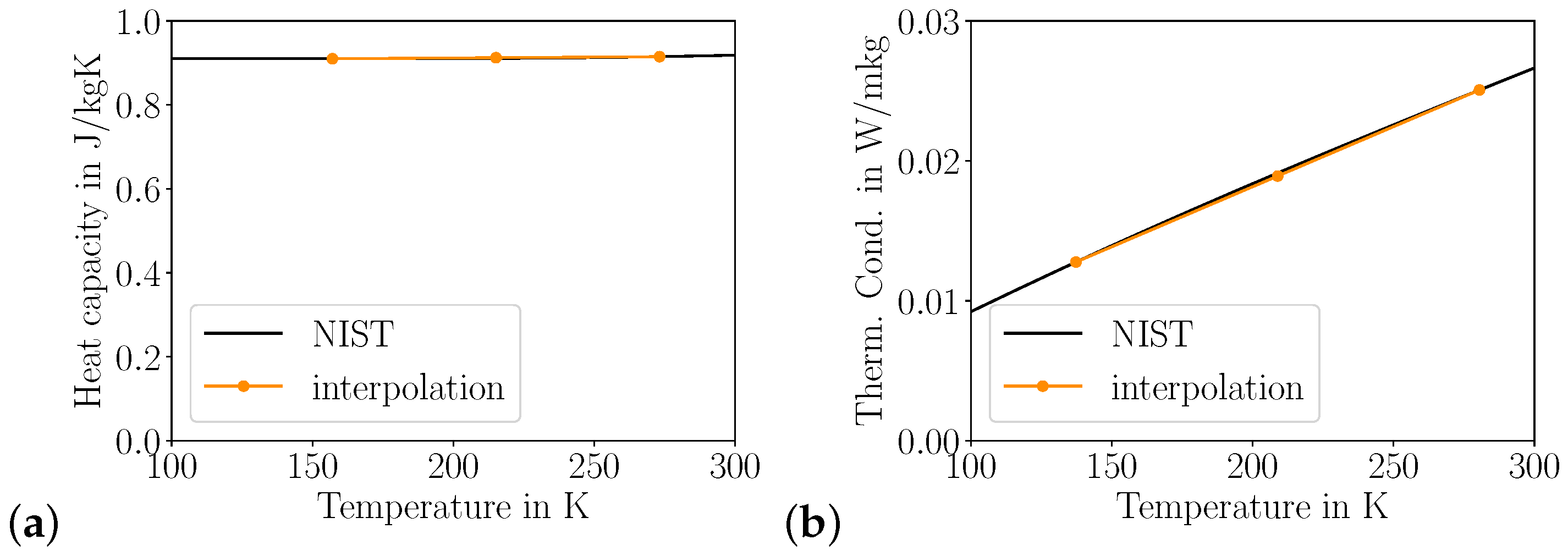
2.1. Fluid Properties

Real fluid properties, such as shown in Figure 1, are characterized by striking nonlinear deviations from ideal fluid models. Generally, we can distinguish thermal, caloric, and transport properties. The thermal equation of state relates pressure p, density ρ , and temperature T of a fluid. The caloric EOS relates fluid energy (e.g., enthalpy) to p v T . Finally, transport properties, such as viscosity or thermal conductivity are not directly linked to any EOS and mostly stand-alone correlations.
Here, we use the cubic equations of state developed by Peng and Robinson [27] (PR) and Soave, Redlich, and Kwong [28] (SRK). Cubic EOS are comparatively cheap computationally, but not very accurate. Today, high-accuracy reference EOS are typically based on expressions of the Helmholtz free energy [39]. These equations have been reported countless times and will thus not be repeated here.
It is important to note that the functional form of either approach has no physical relevance [39]. Cubic equations of state are arbitrary extensions of the van der Waal EOS [40]; Helmholtz EOS were developed because relevant fluid properties can be obtained through differentiation rather than integration from the Helmholtz free energy, increasing the flexibility and hence accuracy significantly. Thus, there is no fundamental advantage of these EOS over other fluid property representations, such as neural networks [33,41].
Here, we will use the CoolProp library [34] and NIST database [38] to determine baseline fluid properties using the aforementioned EOS.
The mixture critical point will be evaluated using the pseudo-critical method [42,43], where the effective mixture critical properties are computed based on the composition and the pure fluid properties.

2.2. Computational Fluid Dynamics

We used the open source CFD library SU2 [44] with its low-Mach number approximation solver [45] for simulations in this paper. We extended the solver to use tiny neural networks (TNN) for efficient and accurate fluid property modeling [33,41,46]. A thorough discussion is given in Longmire and Banuti [33] and will be omitted here.
Artificial neural networks are used to model the fluid’s density ρ , isobaric specific heat capacity c p , isochoric specific heat capacity c v , thermal conductivity k, and viscosity μ shown in Figure 3. The ANN models match the NIST data well; the Peng–Robinson equation of state overestimates the low-temperature density and underestimates the maximum isobaric specific heat capacity by about 20%. We chose CO 2 because, from the species compared in Figure 4, carbon dioxide shows the smallest bias for either SRK or PR accuracy, while still being relevant for rocket engines.

3. Results

In this section, we discuss (1) property representation errors and show how they impact real fluid simulations; (2) sampling errors as a numerical error type not encountered in gas or liquid flow simulations.
In particular, we focus on the common propellants oxygen and methane, and the main combustion products carbon dioxide and water. The chosen pressures represent technically relevant cases of near-critical experiments (6/7 MPa), gas generator cycles (10 MPa), and staged combustion cycles (20 MPa).

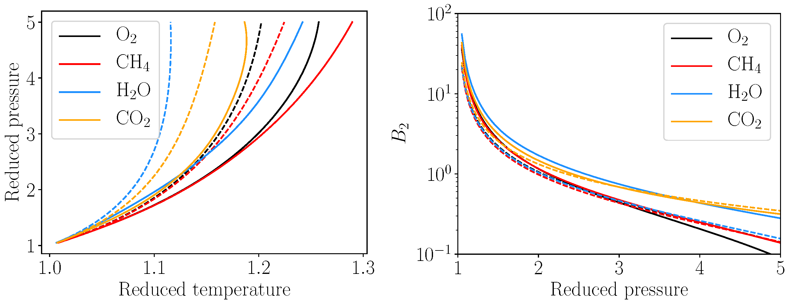
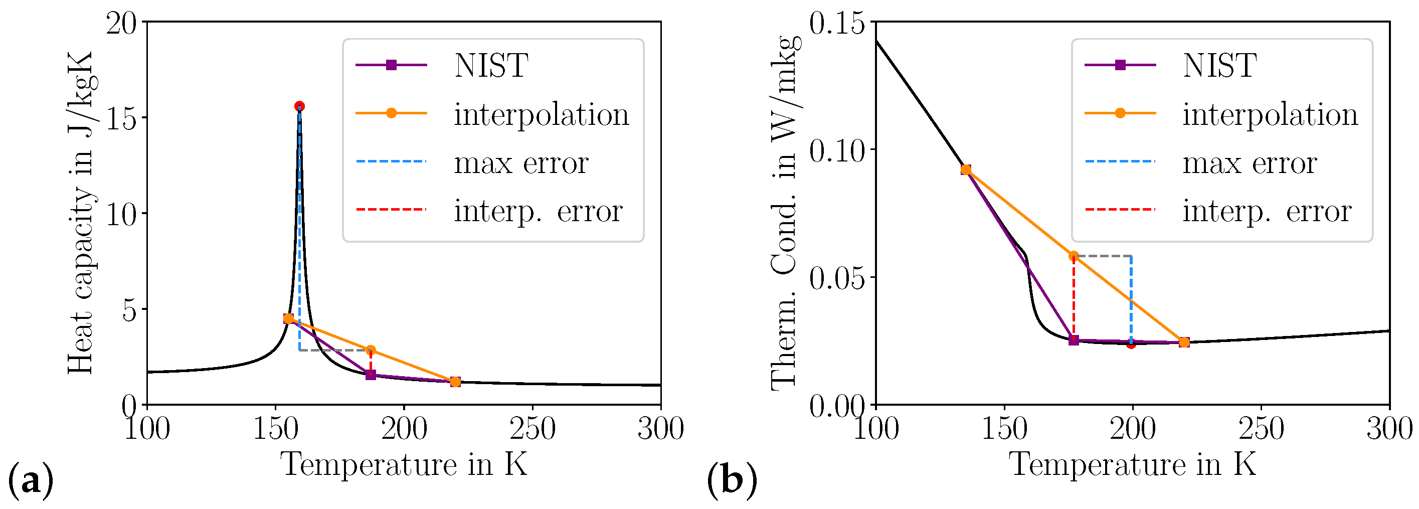
3.1. Property Representation Error

The most striking effect of real fluid property models is, naturally, their difference to idealized models for ideal gases ( p = ρ R T ), or incompressible fluids ( ρ = const ). In this section we will discuss the magnitude and impact of inaccurate fluid property models, e.g., by using cubic EOS. Naturally, this aspect has been investigated since the advent of the very first real fluid CFD models [23]. It is long known that cubic EOS may introduce, e.g., errors in density of 10% to 20%.
Here, we will discuss the relevance of the density and the isobaric specific heat capacity.

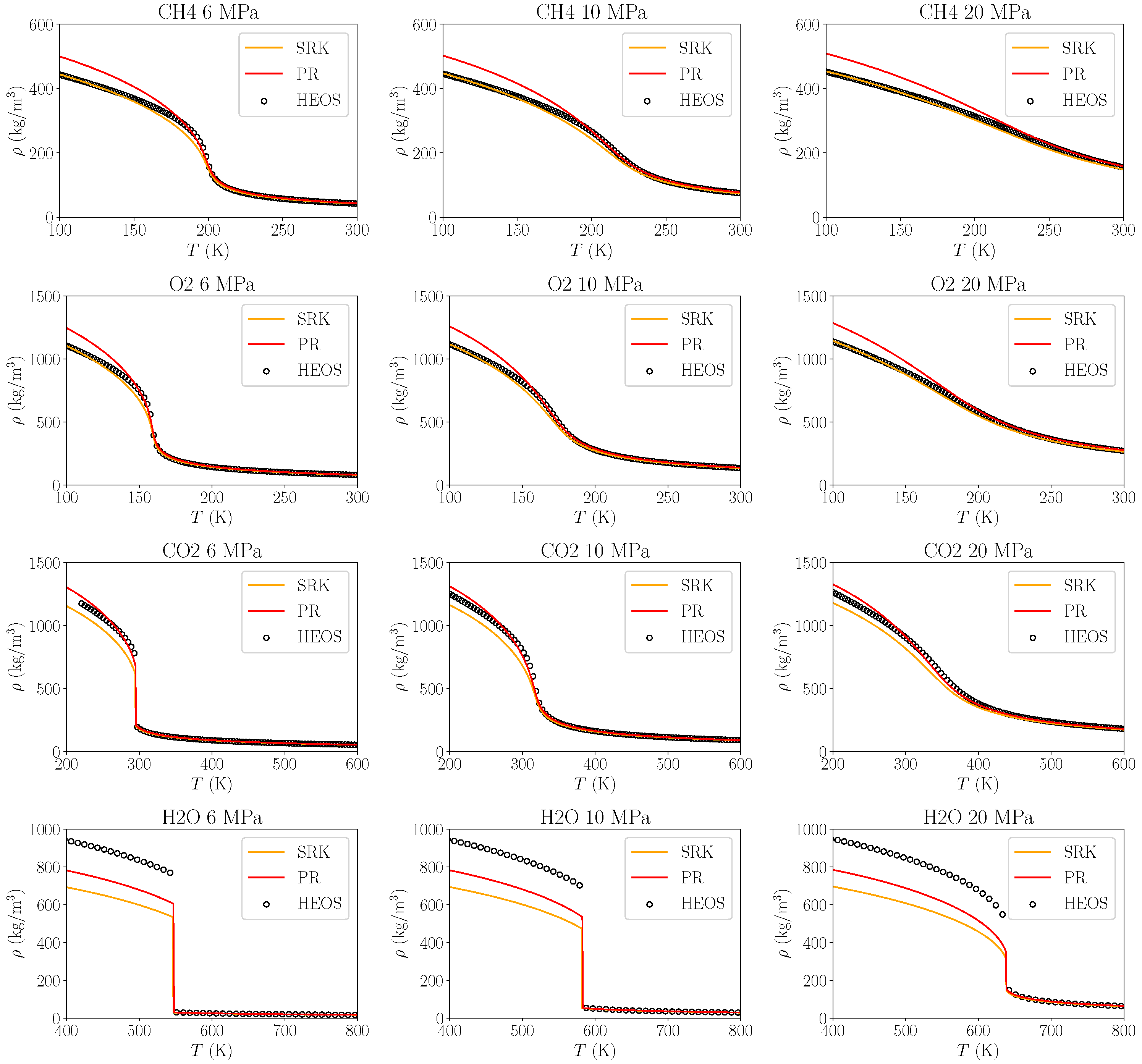
3.1.1. Density Errors

Why is the density relevant? The jet break-up length and thus position of heat release in coaxial injectors, where an inner jet is surrounded by an annular flow and their respective injection velocities u, scales mostly with the momentum flux ratio between both streams,
J = ( ρ u 2 ) outer ( ρ u 2 ) inner .
On the other hand, the global chamber conditions are mostly determined by the overall oxidizer-fuel ratio O F R ,
O F R = m ˙ Oxidizer m ˙ Fuel = ( ρ u A ) Oxidizer ( ρ u A ) Fuel ,
where A is the injector area.
If we do not get the density right in our simulations, we cannot capture both the overall chamber conditions such as temperature or speed of sound and the correct propellant jet break-up and heat release. However, both are essential parameters for combustion instabilities [2]. Figure 4 compares reference quality data for density ρ at rocket-relevant conditions 6, 10, and 20 MPa, for the rocket-relevant species methane, oxygen, carbon dioxide, and water.
It becomes clear that cubic EOS always involve a trade-off: SRK data is more accurate towards lower temperatures for the propellants oxygen and methane, but PR captures the liquid–gas transition much better. For the reaction products carbon dioxide and water PR data seems slightly better, but we have to conclude that neither cubic EOS can represent the fluid properties accurately.

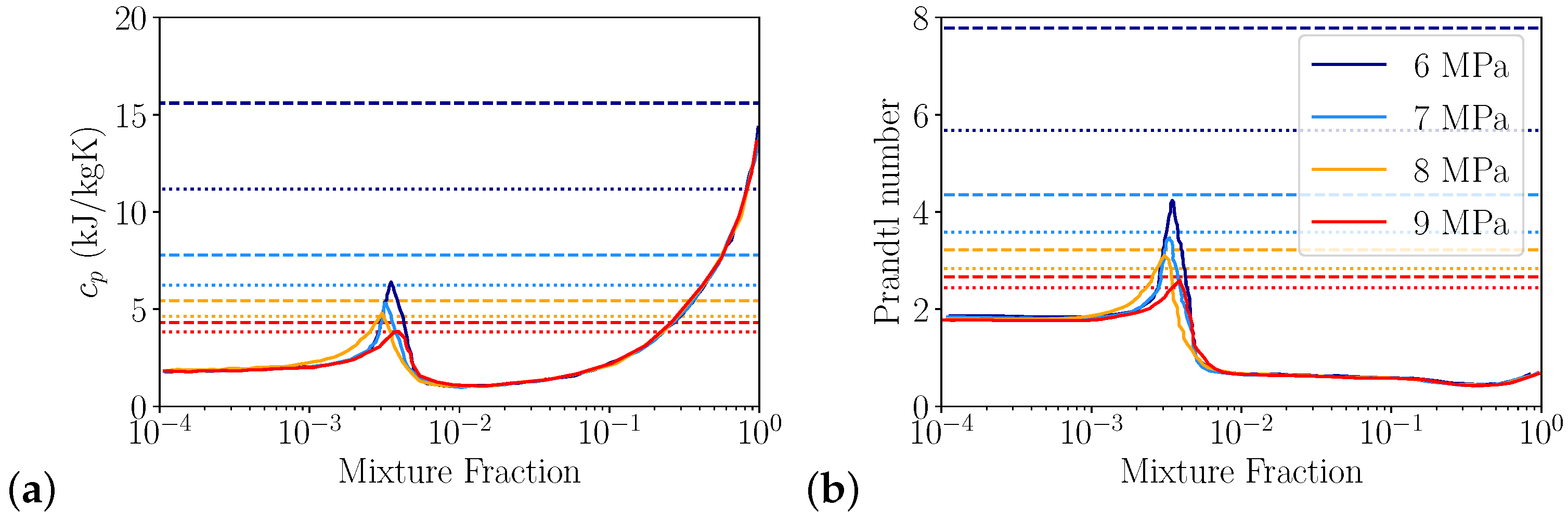
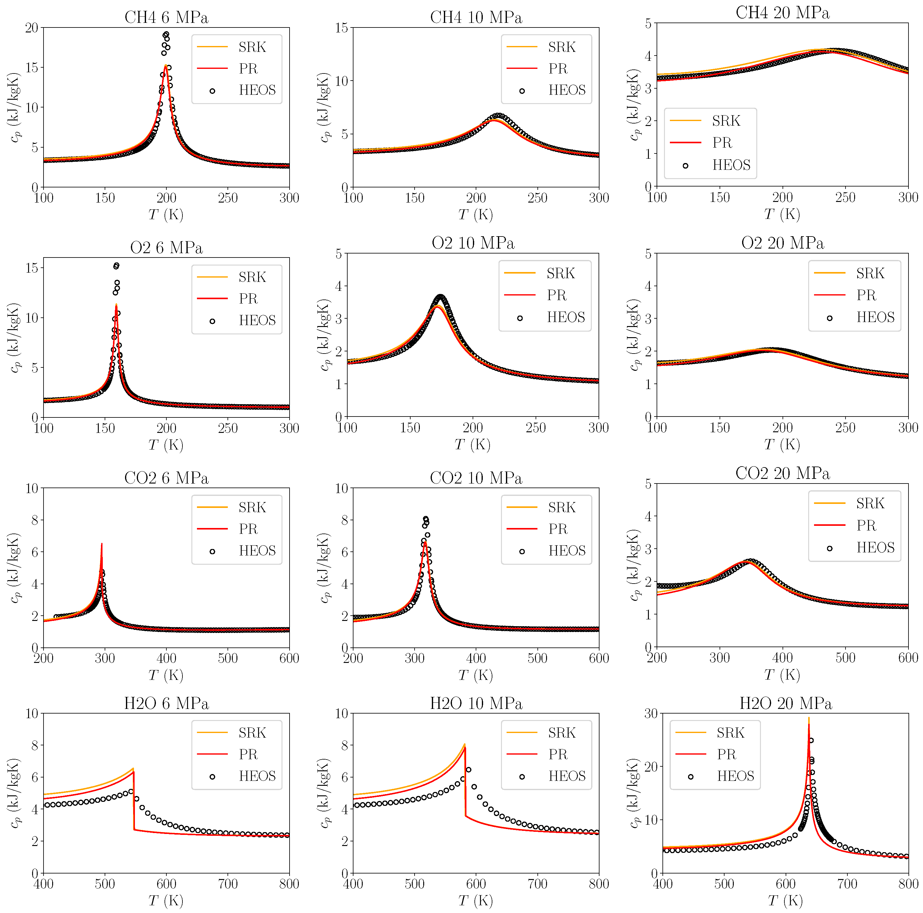
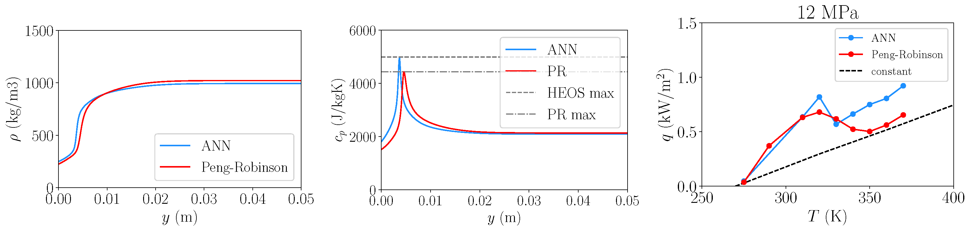
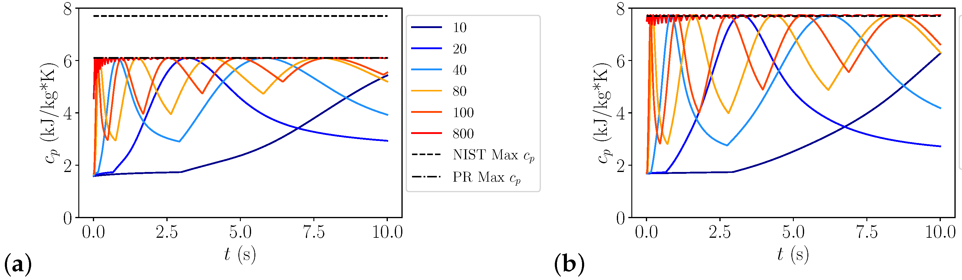
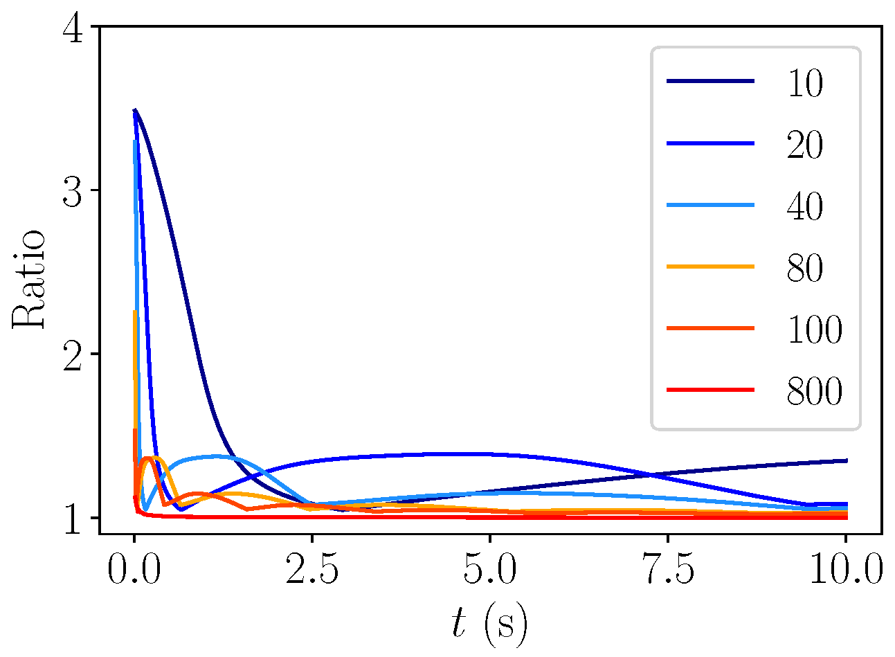
3.1.2. Heat Capacity Errors

The isobaric specific heat capacity c p plays a more indirect, yet equally important role for propellants. Figure 1 shows the distinct peak in heat capacity, which represents the pseudo boiling condition [29], marking the position of maximum change during the supercritical liquid–gas transition.

Heat Transfer

On the one hand, c p is a dominating factor in the calculation of the Prandtl number Pr, c.f. Figure 1, which in turn governs transient heat transfer. Figure 1 furthermore shows the dramatic local peak in Pr which is manifest as a layer of locally high Pr in a fluid exhibiting a temperature distribution across pseudo boiling, and acting as an insulator that inhibits heat transfer across that layer.
Figure 5 compares reference quality data for c p at rocket-relevant conditions 6, 10, and 20 MPa, for the rocket-relevant species methane, oxygen, carbon dioxide, and water. Particularly at low supercritical pressures, reference data exceed cubic EOS data by as much as 30%. The difference between PR and SRK EOS is less pronounced for the heat capacity compared to density data.
Generally, an underestimated Pr leads to an overestimated heat transfer rate. Thus, the insulating properties of the pseudo boiling layer will not be reflected in our simulation if our fluid property model misses that value by 30%.

Pseudo Boiling

Another important aspect of the heat capacity peak is its physical meaning as a supercritical latent heat [29,30]. Ernst Schmidt was the first to realize [48,49] that the widening heat capacity distribution around saturation conditions at high subcritical pressures plays the role of a distributed latent heat. This can be seen in Figure 5 for water, where a more and more pronounced peak and tail of c p are developed for increasing subcritical pressures. We now understand that this view can be extended to supercritical pressures [29,30], where the instantaneous latent heat has been completely replaced by the wide c p peak. Somewhat surprisingly, the integral of the c p across the complete transition is invariant for a wide range of pressures, establishing a generalized latent heat that can be identified for both subcritical and supercritical transitions.
This naturally leads to the questions of whether cubic EOS capture the location and the strength of the pseudo boiling transition. We understand the transition location as the temperature at which the heat capacity and the isobaric thermal density gradient reach maxima [29]; we understand the strength in terms of the boiling number B 2 [29], which measures the height of the c p peak in relation to the limit value towards liquid conditions at lower temperatures. This becomes intuitively clear when regarding oxygen data in Figure 4 and Figure 5: at low pressures, we see a distinct drop in density to occur simultaneously with the heat capacity peak. At higher pressures, this transition has moved to higher temperatures while becoming much less pronounced.
Figure 6 shows that cubic EOS are not good at capturing the pseudo boiling transition. For the regarded species, they generally predict the transition to occur at temperatures that are too low (for the case of water at a reduced pressure of 5 by 80 K). The magnitude measured by B 2 is systematically underpredicted at lower reduced pressures. At reduced pressures exceeding 3, it depends strongly on the species: PR data matches reference data well for carbon dioxide; however, identical distributions are predicted for oxygen, methane, and water, even though the reference data shows distinct curves.
We have to conclude that cubic EOS simultaneously overestimate heat transfer to a transcritical fluid, underestimate the amount of energy needed to transform it to a gaseous state during the transition (i.e., heat capacity peak), and predict the wrong temperature at which this transition should occur. This suggests that cubic EOS will tend to underestimate the timescale of pseudo boiling processes, such as the thermal break-up of transcritical jets [32], the vaporization of transcritical droplets, or the formation of vapor layers during film boiling [33].

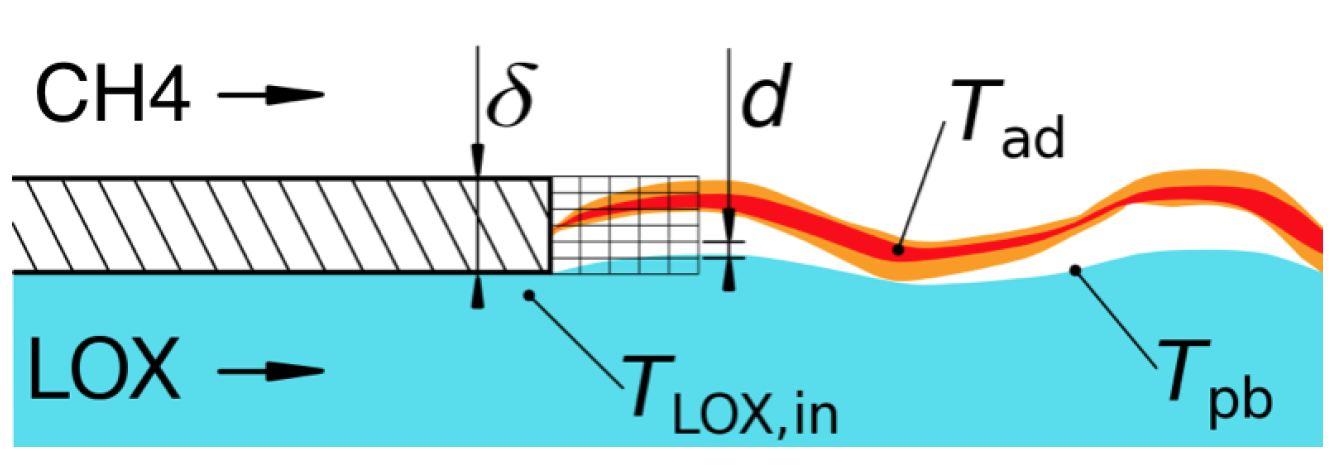
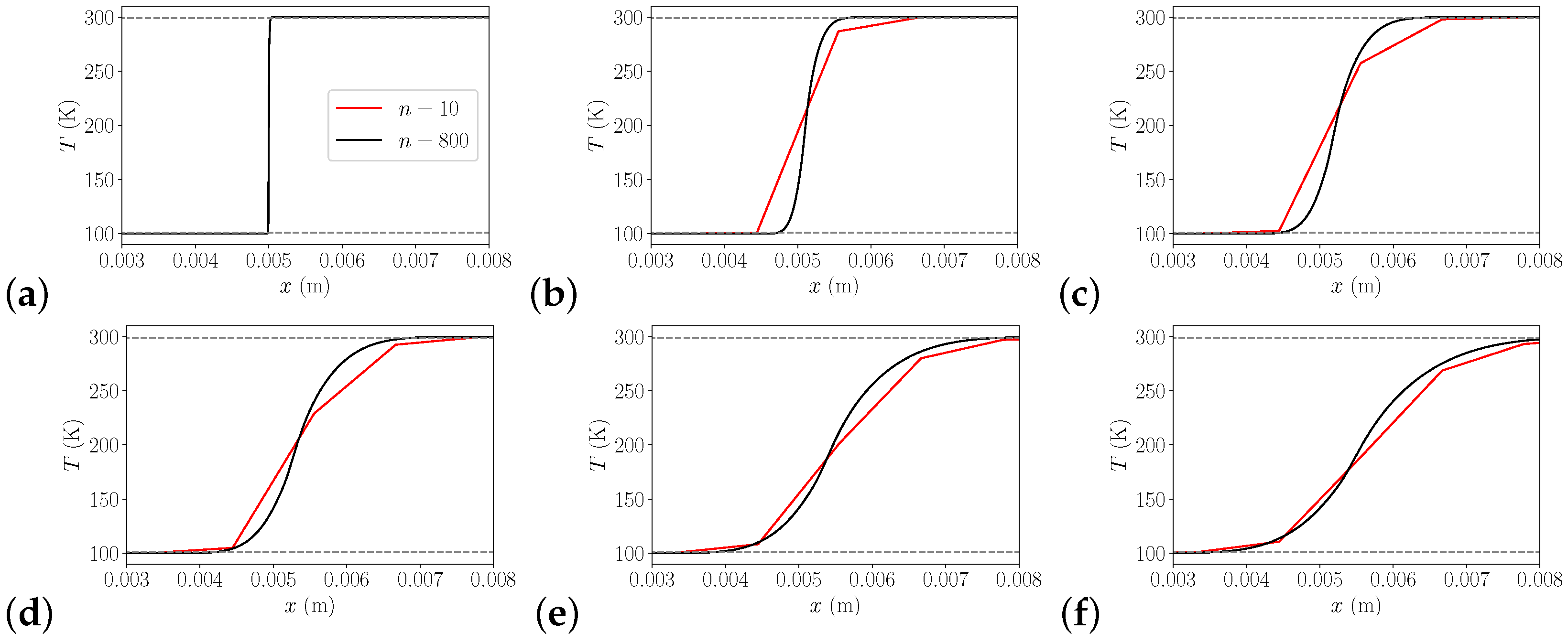
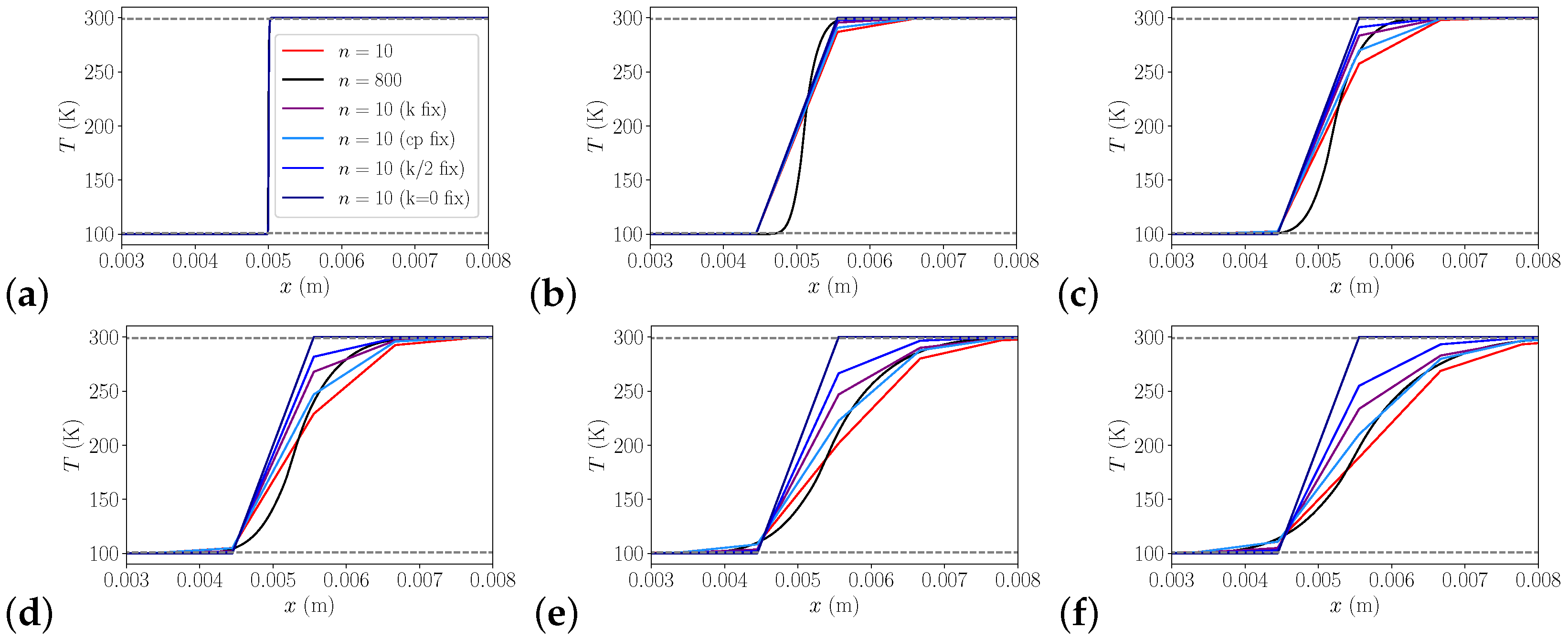
3.1.3. 2D Heat Transfer
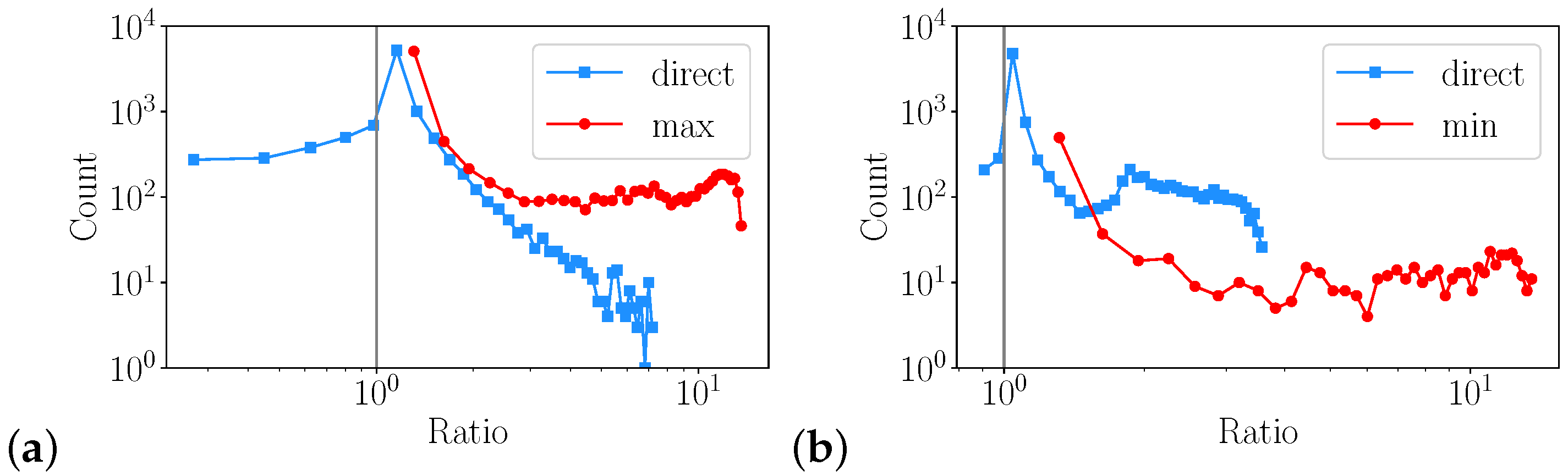
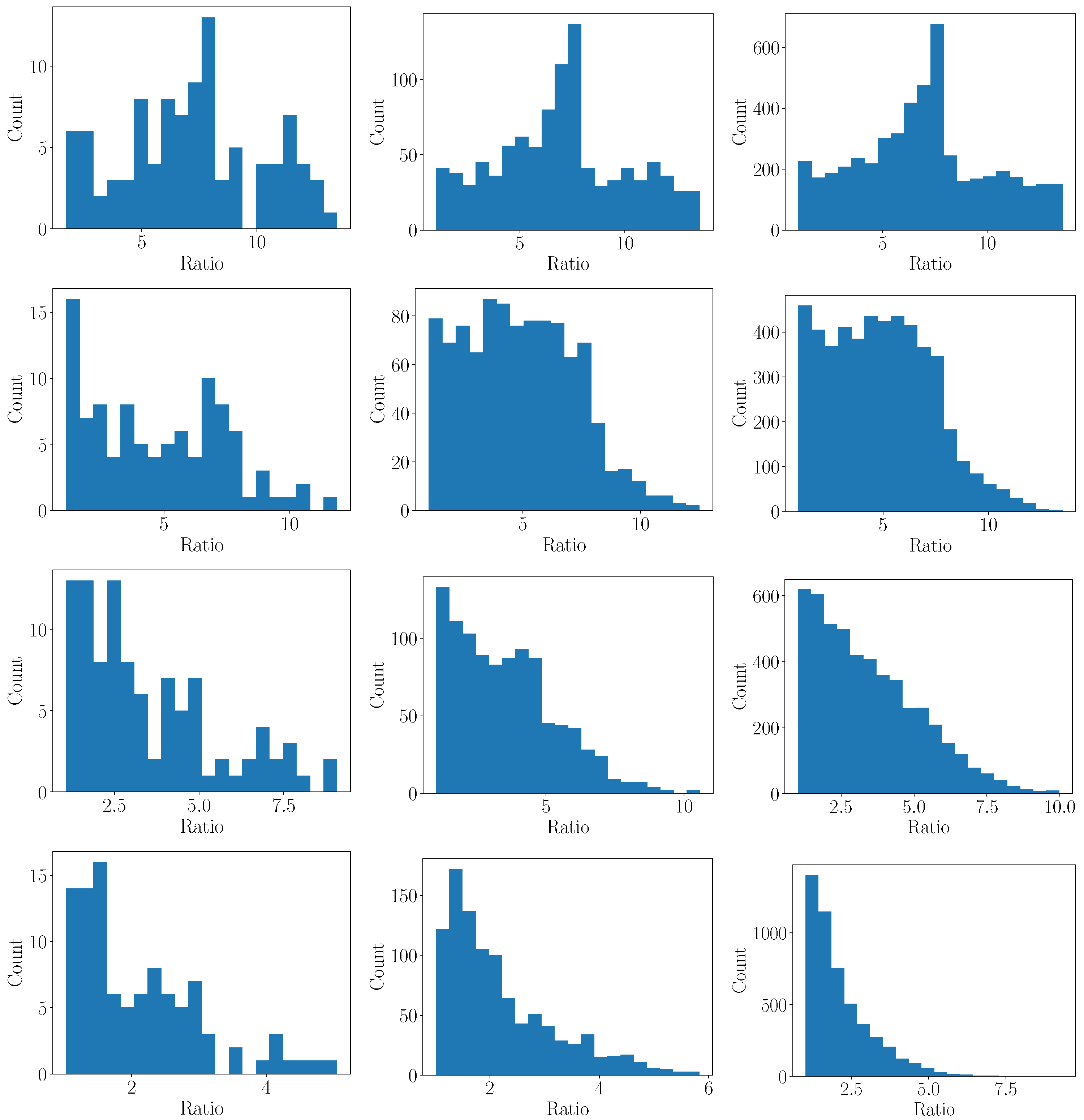
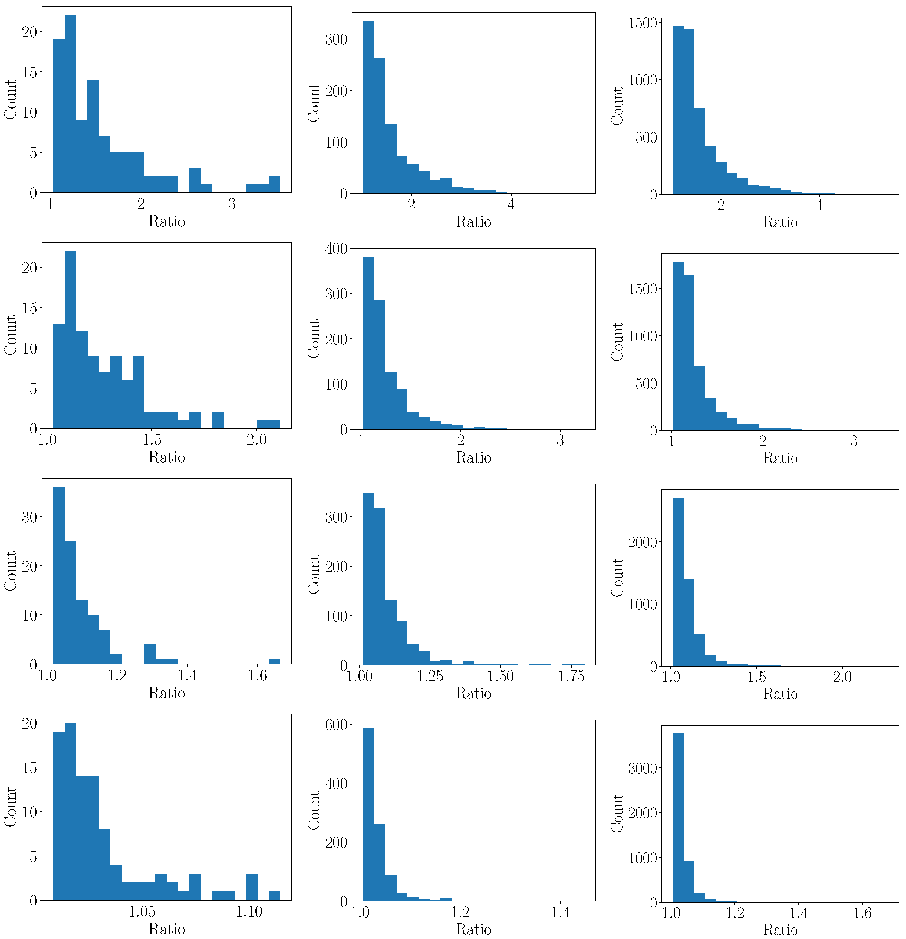
To show the importance of the EOS and how it impacts the results of simulations, compared the results of the highly accurate TNN shown in Figure 3 to the Peng–Robinson EOS in a parameter study of supercritical CO 2 of a laminar heated flat plate. We chose CO 2 because, from the species compared in Figure 4, carbon dioxide shows the smallest bias for either SRK or PR accuracy, while still being relevant for rocket engines. An in depth explanation of an original test case can be found in [33]. At a Reynolds number of Re = 112 and at a bulk temperature of T = 270 K, we set the wall temperature to different temperatures, at and above pseudo boiling which heated the bulk fluid. These simulations were performed for two different pressures of p = 12 , 20 MPa, and for two different EOS using the ANN and a second time using the PR EOS. To compare the results boundary layer profiles were taken and the heat flux along wall for each simulation was extracted to create a boiling curve.
The plot in Figure 7 is a density contour plot for the simulation with a wall temperature of T w = 390 K. The contour plot shows a steep density change for the fluid close to wall as a thin vapor film forms close to the wall.
Figure 8 compares the density ρ in the boundary layer and the isobaric heat capacity c p in the boundary layer for the results using the two different EOS. The top are the results for the 12 MPa case with T w = 390 and the bottom are results for the 20 MPa case with T w = 390 . The density boundary layer plots show that the PR EOS over predicts the liquid density in the bulk fluid while also showing a larger thickness of the vapor film near the wall. The heat capacity plots show the PR EOS under predicts the maximum heat capacity while also being offset from the TNN results.
Figure 8 further compares the heat transfer results of the different EOS for the two different pressures. The plots show the average heat along the wall for each wall temperature which is a boiling curve. There is little to no variation in the heat transfer results for wall temperatures that are close to the bulk fluid temperature because there is little to no variation in the fluid properties but as the wall temperature increases there is large variation between the simulations using the two different EOS. For the 12 MPa case the ANN show a larger local maximum compared to the PR EOS and as the wall temperature increases more the PR EOS under predicts the rate of heat transfer compared to the highly accurate ANN models.
The simulation reveals that the introductory remark of an underestimated Prandtl number and supercritical latent heat do not necessarily lead to direct decrease in heat transfer. Here, Figure 8 shows that this is indeed the case for low wall temperatures. However, as a result, an insulating wall vapor layer can more easily form and inhibit further heat transfer. Case in point, PR underestimates the maximum heat transfer, overestimates the vapor layer thickness, and overall predicts a more smooth transition to heat transfer deterioration.

3.2. Sampling Error

We have addressed the extent and impact of inaccurate fluid properties as derived from using cubic equations of state. However, our opening example in Figure 2 highlights another potential source or error, one that, to the best of our knowledge, has not received any attention so far.
Consider the cartoon of the flow field behind a coaxial injector in Figure 9. Behind a LOX post of thickness δ , streams of gaseous methane and liquid oxygen meet, mix, and react. We can identify the adiabatic flame temperature T ad as the maximum temperature reached in the field. Following the path of oxygen [50], it is injected with a temperature T LOX , in , heats through pseudo boiling at T pb , before mixing and reacting. With flames mostly anchored behind the LOX post [7,12], this means that the flow behind the LOX post sees a temperature increase from ≈100 K in the LOX stream to ≈3500 K in the flame, or to ≈300 K in an ambient temperature gaseous methane stream.
If we want our solvers to capture the extremely narrow c p peak maximum, we need a mesh of sufficiently small cells of size d to ensure a ≈1 K temperature resolution, over a δ width space. As a naive order of magnitude evaluation, to resolve a 1 K interval over the 200 K temperature difference during inert mixing, we will need O ( 100 ) cells. However, as this assumes a perfectly regular distribution of both mesh resolution and temperature, the actual number to ensure capturing even under adverse conditions will likely be higher. If the mesh is insufficiently resolved, our method will not be able to capture the relevant fluid property. This is what happens in Figure 2, where even the extremely fine mesh skips over the c p peaks.
We will refer to this as sampling error. The simplest configuration to potentially exhibit this sampling error is a 1D temperature difference. In the following, we discuss two fundamentally different approaches to quantify the impact of a sampling error: First, a Monte Carlo approach that is solver agnostic; second, a 1D transport problem evaluated in the open source SU2 solver. The overall strategy in both cases is to locally extract the heat capacity and transport properties directly on the mesh, in order to quantify how often extrema in transport properties are skipped by the solver, and what the corresponding errors are.

3.2.1. Monte Carlo

The idea behind our Monte Carlo transport analysis is that on a computational mesh capturing some state and property, the precise location of a particular state on a grid point is essentially random. For a sufficiently resolved simulation, the form of the underlying mesh should be irrelevant; the flow may additionally move across the mesh so that locally resolved states change temporally and spatially.
This is not an issue for fluids with moderate or smooth property variations, such as ideal gases or liquids. Figure 10 shows how linear interpolation from certain discrete points can be used as very good approximations for the actual physical property between the sampled points, using oxygen data from the NIST database [38] at p = 0.01 MPa.
However, for transcritical flows, two complications need to be accounted for when regarding fluid properties in adjacent cells: First, fluid property curves may exhibit a local curvature that introduces a significant error if a fluid property is estimated from linear interpolation or distinct local extrema are present that cannot be recovered from averaging and require for a mesh point to reach the exact state of the extremum. Second, it is these extrema rather than local or averaged property values that may constrain transport fluxes, and thus act as a bottle neck.
Figure 11 shows how the isobaric specific heat capacity and thermal conductivity for a near-critical fluid (oxygen at 6 MPa) exhibit this structure that is extremely challenging to sample accurately. In both cases, the value obtained from interpolation deviates by more than a factor of two from the actual value at the point of interest; for c p , the error compared to the maximum value in the respective temperature interval is, however, much larger.
We have two core concepts to this Monte Carlo transport analysis:
1
Within bounds defined by the boundary conditions, states can be randomly sampled from the physical fluid properties to obtain information about how numerical properties are reconstructed on a discrete representation.
2
Extremal values of fluid properties that minimize transport need to be taken into account as they act as bottle necks.
As an example, the evaluation shown in Figure 11 is performed 10,000 times, i.e., within the boundary conditions 100 K and 300 K, two random temperatures are determined following a uniform distribution, then the relevant physical ( ϕ ), interpolated ( ϕ ¯ ), and extremal values ϕ ext are identified. Figure 12 shows the results, where the direct error is the ratio of physical and interpolated values, and max/min are the ratios of the interpolated and the extremal values.
For the specific heat capacity in Figure 11a, the majority of cases do find a ratio close to unity when random temperatures are sampled that are close together or far away from the extremum, such that a linear interpolation is a close approximation. Because the second derivative of c p is mostly positive except for the narrow region around the peak, the interpolation overestimates the value except when the peak is enclosed, such that the peak in the histogram for the direct error in Figure 11a is moved to a value slightly larger than unity. Over all, we see that the simple interpolation may be wrong by more than an order of magnitude, with a higher error when compared to the extremum. The same pattern can be seen in Figure 11b for the thermal conductivity.
We find that for two randomly sampled mesh temperatures, there is indeed a substantial error to the physical property to be sampled based on the unique structure of supercritical fluid properties—something not observed for ideal gases or liquids. The previous analysis, however, has the shortcoming of not being mesh-size sensitive. In the following, we thus extend the study to account for a provided mesh resolution. In order to quantify mesh resolution effects, an extended study is performed using the following steps:
1
Prescribe a mesh resolution n and the boundary conditions T min and T max .
2
Determine n 1 random temperatures (uniform distribution) in the interval [ T min , T max ] . Together with the boundary conditions T min and T max , n temperature intervals are thus identified.
3
For each interval, perform the analysis illustrated in Figure 11.
4
Save the maximum error obtained across all intervals [ T min , T max ] .
5
Repeat the above steps N times to analyze a distribution of the error for a given resolution n.
6
Repeat the above steps for different n to study the impact of the resolution.
Figure 13 and Figure 14 show the results of an evaluation of the heat capacity c p for temperature boundary conditions of 100 K and 300 K, for mesh resolutions n of 4 to 800 cells, with different numbers of sample runs N from 100 to 5000. It can be seen that N = 1000 samples already give a good estimate of the final result.
For the coarse meshes in Figure 13 the ratios between the maximum value and the numerical value may by as high as a factor of ten. Even for 50 cells, a significant number of samples will estimate numerical values that are more than a factor of 2 from the physical values. Towards higher resolution, this effect gets smaller and smaller. Figure 14 shows that errors are mostly below 10 % for a resolution of 800 cells.

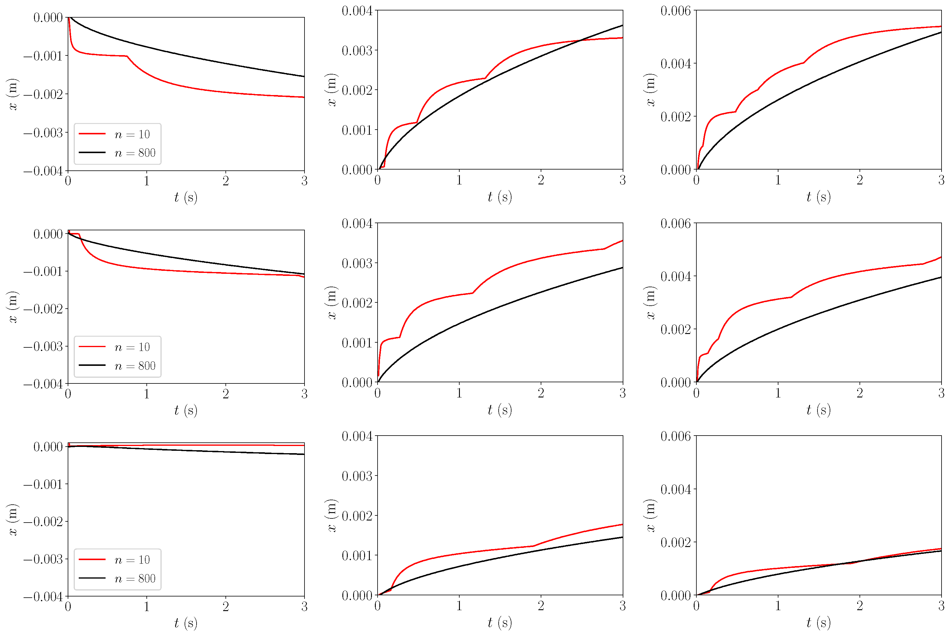
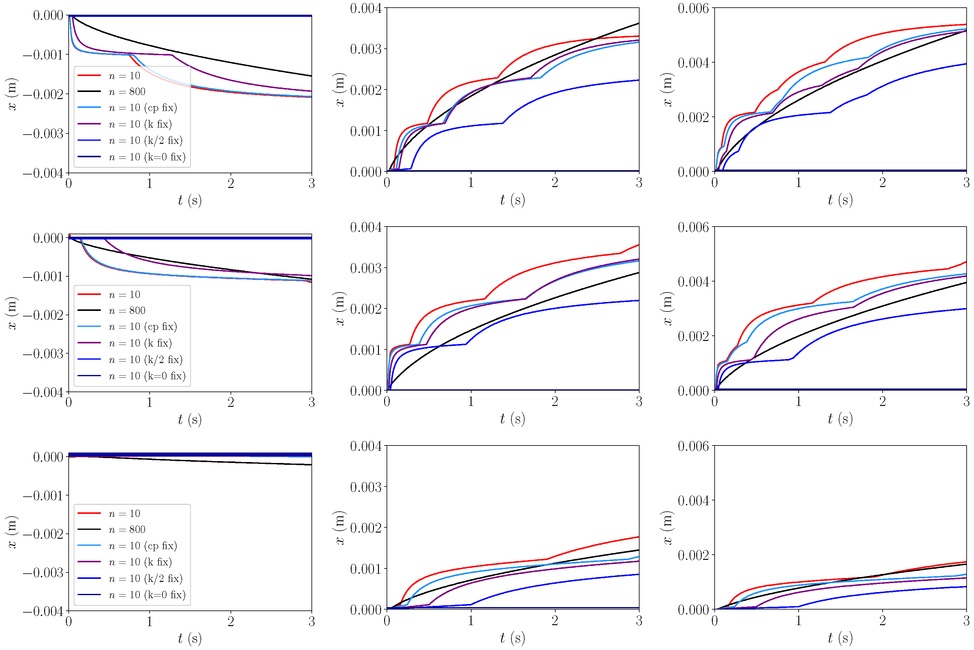
3.2.2. 1D Heat Transfer

The other test case to demonstrate the discretization error is a 1D transport problem. Specifically, the chosen test case is split between a cool liquid-like side and a warm gas-like side. The temperature difference of the the two sides will induce a heat flux. The fluid of interest here is oxygen at 7 MPa. Artificial neural networks were used to model the fluid properties [41,47]. The computational domain is 1 cm long; six different mesh resolutions were used n = { 10 , 20 , 40 , 80 , 100 , 800 } . The goal of the 1D mixing case is to assess whether there is a clear difference in transport between the coarse and the fine meshes.
The case is set up so that there is a cold liquid-like side on one half of the domain, and a warm gas-like state on the other side, where the temperature difference induces a heat flux. The fluid for the 1D heat transfer case is oxygen at 7 MPa ( p r = 1.389 ). The cold liquid-like oxygen is initially set to a temperature of 100 K as this temperature is before pseudo boiling, and the warm gas-like oxygen has an initial temperature of 300 K which is a temperature above pseudo boiling. The pseudo boiling temperature for oxygen is at 163 K, so the fluid goes through the pseudo boiling process during the heating process. The computational domain is 10 mm long. The elements are equidistant, and six different mesh resolutions were used where n is the number of elements n = { 10 , 20 , 40 , 80 , 100 , 800 } . The number of elements and grid spacing is shown in Table 2. The top and bottom boundaries of the domain are Euler walls, and the left and right boundaries of the domain are pressure boundaries that are set so there is no back pressure. The time simulated is 10 s; the spreading interfacial layer reaches the boundaries after about 3 s.
Physically, as the density interface moves through the fluid, the c p peak associated with pseudo boiling is present at each point in time.
For the different meshes, c p in each cell is calculated using the temperature, and the maximum c p throughout the computational domain for each time step is taken and plotted as seen in Figure 15. The plot shows that only the most refined mesh of 800 elements fully recovers the maximum of the isobaric heat capacity. In contrast, the coarser meshes only capture the maximum periodically and randomly throughout the simulation. Since the coarser meshes underestimate the maximum c p , it is expected that the heat transfer rate would be faster in the coarser meshes. None of the meshes can recover the NIST maximum of the isobaric heat capacity fully for the plot on the right, but this is due to the Peng–Robinson fluid property model as it underestimates the maximum isobaric heat capacity by about 20%.
Further, for each mesh at each time step, the mean thermal conductivity is calculated between each cell and compared to what the NIST thermal conductivity would be based on the mean temperature between each cell. A ratio between the simulation value and the NIST value was calculated, and the maximum ratio was taken for each time step and plotted, shown in Figure 16. For the coarse meshes, the ratios are large, meaning there is a significant error between the simulation value and the NIST value. The error decreases as the number of elements in the mesh increases, and the curves converge because more points are available at later timesteps. The error is negligible in the most refined mesh of 800 elements as the ratio between the simulation value, and the NIST value is 1. This shows that for the coarse meshes, the solver overestimates the mean thermal conductivity compared to the fine meshes, again indicating that the heat transfer in the coarse meshes should occur at a faster rate than in a fine mesh.
The spreading of the interface is shown in Figure 17. At t = 0 , the left half of the domain is 100 K, and the right half of the domain is 300 K. As time goes on, the liquid and gaseous oxygen will mix, and the temperature curve will begin to flatten until eventually a linear distribution of the temperature is reached. The plot shows that the heat moves faster in the coarse mesh than in the fine mesh.
To better quantify and analyze the movement of the heat, the position of a high and low-temperature threshold is tracked. As time increases, this high temperature threshold will move, and its x position will increase, and the low temperature threshold x position will decrease. How fast these positions change is a measure how quickly the heat moves in each simulation. Figure 18 shows the results of this analysis and compares the difference of the results between a coarse mesh of 10 elements and a fine mesh of 800 elements. The change of the position of the low temperature and high temperature thresholds show that the thresholds move faster in the coarse mesh than in the fine mesh.
Sampling error on practical meshes cause the thermal conductivity to be overestimated, and the isobaric heat capacity to be underestimated. To counter act the overestimation and underestimation, fixes to the thermal conductivity and isobaric heat capacity models are applied. The overall strategy is to ensure that the extrema values of c p and k are preserved. For the thermal conductivity three fixes are demonstrated. For the first, two adjacent cells’ temperature are checked; if the left cell is above 154 K and the right cell is below 300 K, the minimum thermal conductivity between the two cells is used instead of calculating the mean thermal conductivity between the two cells.
k = min ( k i , k j ) if T i > 154 K T j < 300 K ; k i + k j 2 otherwise .
For the second fix, two adjacent cells’ temperature are checked; if the left cell is above 154 K and the right cell is below 300 K, the half of the minimum thermal conductivity between the two cells is used instead of calculating the mean thermal conductivity between the two cells.
k = min ( k i , k j ) 2 if T i > 154 K T j < 300 K ; k i + k j 2 otherwise .
For the third fix, two adjacent cells’ temperature are checked; if the left cell is above 154 K and the right cell is below 300 K, the thermal conductivity is set to zero.
k = 0 if T i > 154 K T j < 300 K ; k i + k j 2 otherwise .
For the isobaric heat capacity fix, the temperature in each cell is checked, and if the cell’s temperature is in the range of 154 K to 170 K, the heat capacity is set to the maximum value of 7641 J/kgK.
c p = c p m a x if T i > 154 K T j < 170 K ; ANN value otherwise .
Figure 19 are plots of the temperature along the domain at different time steps. These plots show that the cases on the coarse mesh with the c p fix and the case with the k in Equation (3), the heat moves at a slower rate than the coarse mesh with no property fix, but the heat is moving faster than in the case using the fine mesh. The cases with the other k fixes move slower than both the coarse mesh and the fine mesh.
Again to better quantify and analyze the movement of the heat in the flow, the position of a high and low temperature threshold is tracked. As time increases, this high temperature threshold will move, and its x position will increase, and the low temperature threshold x position will decrease. Figure 20 shows the results of this analysis and compares the difference of the results between a coarse mesh of 10 elements, a fine mesh of 800 elements, a coarse mesh of 10 elements with three different fixes to the thermal conductivity k, and a coarse mesh of 10 elements with a fix to the isobaric heat capacity. For the movement of the low temperature threshold, the case on the coarse mesh with no property correction and the case with the c p fix were very similar. Furthermore, the movement for the low temperature threshold shows that the case with the k fix using Equation (3) moves slower than the coarse mesh case with no correction but faster than the fine mesh, but the cases using the other two fixes to the thermal conductivity, the heat moves faster than the coarse and fine mesh. The movement of the high temperature threshold shows the same thing as the low temperature threshold. The difference between the low and high temperature threshold movement shows that the heat transfer is slower for the case with the c p fix and the case with the k fix using Equation (3) than the coarse mesh, but the heat transfer is faster for these cases than the case using the fine mesh. Furthermore, the plots show that the cases with the other two k fixes, the heat moves slower than both the coarse mesh and the fine mesh. The difference between the low and high temperature threshold movement also shows that the heat transfer for the cases with the k fixes are slower than the case with the c p fix.

4. Conclusions

The present analysis showed that property representation of near-critical fluids (e.g., heat capacity, thermal conductivity, viscosity) in a solver is strongly affected and degraded by the highly nonlinear and non-monotonous fluid behavior. In particular, the estimation of inter-cell properties, such as a mean thermal conductivity, may yield values that exceed physical values by multiples.
For heat conduction, the relevant properties (heat capacity, thermal conductivity) yield errors that always lead to an overestimation of heat conduction predictions. This may have an impact on predictions of regenerative cooling, wall heat flux for film cooling, or liquid core length determinations for injection simulations.
Effectively, this behavior introduces a new—thermodynamic—mesh resolution requirement in addition to classical constraints such as y + or Kolmogorov length scales. Two different methods of estimation (Monte Carlo, 1D CFD) show that a O ( 800 ) point resolution is required to accurately capture the extremal fluid properties in supercritical oxygen for the temperature interval 100-300 K. Consider the LOX post shown in Figure 9: for cold flow mixing of gaseous CH4 with LOX, 800 cells over a O ( 0.5 mm) width is prohibitive; for reactive flow, the temperature range behind the LOX post is much higher (from cryogenic temperatures, to the adiabatic flame temperature exceeding 3500 K, back to cryogenic temperatures), imposing even higher resolution requirements. Thus, capturing these properties is prohibitive and a model is required.
Finally, our results suggest that previously shown marginal impact of the equation of state may just be a numerical artifact when the solver does not resolve the difference between EOS.

Author Contributions

Conceptualization, D.T.B. and N.P.L.; methodology, D.T.B.; software, N.P.L. and D.T.B.; validation, N.P.L.; resources, D.T.B.; data curation, N.P.L.; writing—original draft preparation, N.P.L. and D.T.B.; writing—review and editing, D.T.B.; visualization, N.P.L.; supervision, D.T.B.; project administration, D.T.B.; funding acquisition, D.T.B. All authors have read and agreed to the published version of the manuscript.

Funding

We gratefully acknowledge the support of NASA MSFC through the Cooperative Agreement 80NSSC20M0256, and of AFRL/RBK through DEPSCoR FA9550-22-1-0306, which funded this research.

Data Availability Statement

The reference data used is publicly available through NIST [38] at https://webbook.nist.gov/chemistry/fluid/ (accessed on 30 August 2022) and CoolProps [34] at http://www.coolprop.org/coolprop/HighLevelAPI.html#propssi-function (accessed on 30 August 2022).

Acknowledgments

We gratefully acknowledge the support of NASA MSFC through the Cooperative Agreement 80NSSC20M0256 which funded this research.

Conflicts of Interest

The authors declare no conflict of interest. The funders had no role in the design of the study; in the collection, analyses, or interpretation of data; in the writing of the manuscript; or in the decision to publish the results.

Abbreviations

The following abbreviations are used in this manuscript:
CFDComputational Fluid Dynamics
EOSEquation Of State
HEOSHelmholtz EOS
SRKSoave Redlich Kwong EOS
PRPeng Robinson EOS

References

  1. Villermaux, E. Mixing and spray formation in coaxial jets. J. Propuls. Power 1998, 14, 807–817. [Google Scholar] [CrossRef]
  2. Yang, V.; Anderson, W. (Eds.) Liquid Rocket Engine Combustion Instability; AIAA: Washington, DC, USA, 1995. [Google Scholar]
  3. Candel, S.; Herding, G.; Synder, R.; Scouflaire, P.; Rolon, C.; Vingert, L.; Habiballah, M.; Grisch, F.; Péalat, M.; Bouchardy, P.; et al. Experimental Investigation of Shear Coaxial Cryogenic Jet Flames. J. Propuls. Power 1998, 14, 826–834. [Google Scholar] [CrossRef]
  4. Delplanque, J.P.; Sirignano, W. Numerical study of the transient vaporization of an oxygen droplet at sub- and super-critical conditions. Int. J. Heat Mass Transf. 1993, 36, 303–314. [Google Scholar] [CrossRef]
  5. Yang, V.; Lin, N.; Shuen, J. Vaporization of Liquid Oxygen (LOX) Droplets in Supercritical Hydrogen Environments. Combust. Sci. Technol. 1994, 97, 247–270. [Google Scholar] [CrossRef]
  6. Sirignano, W.; Delplanque, J.P. Transcritical vaporization of liquid fuels and propellants. J. Propuls. Power 1999, 15, 896–902. [Google Scholar] [CrossRef]
  7. Mayer, W.; Tamura, H. Propellant Injection in a Liquid Oxygen/Gaseous Hydrogen Rocket Engine. J. Propul. Power 1996, 12, 1137–1147. [Google Scholar] [CrossRef]
  8. Mayer, W.; Ivancic, B.; Schik, A.; Hornung, U. Propellant Atomization and Ignition Phenomena in Liquid Oxygen/Gaseous Hydrogen Rocket Combustors. J. Propuls. Power 2001, 17, 794–799. [Google Scholar] [CrossRef]
  9. Oschwald, M.; Schik, A. Supercritical nitrogen free jet investigated by spontaneous Raman scattering. Exp. Fluids 1999, 27, 497–506. [Google Scholar] [CrossRef]
  10. Oschwald, M.; Smith, J.J.; Branam, R.; Hussong, J.; Schik, A.; Chehroudi, B.; Talley, D. Injection of Fluids into Supercritical Environments. Combust. Sci. Technol. 2006, 178, 49–100. [Google Scholar] [CrossRef]
  11. Habiballah, M.; Orain, M.; Grisch, F.; Vingert, L.; Gicquel, P. Experimental studies of high-pressure cryogenic flames on the mascotte facility. Combust. Sci. Technol. 2006, 178, 101–128. [Google Scholar] [CrossRef]
  12. Candel, S.; Juniper, M.; Singla, G.; Scouflaire, P.; Rolon, C. Structures and dynamics of cryogenic flames at supercritical pressure. Combust. Sci. Technol. 2006, 178, 161–192. [Google Scholar] [CrossRef]
  13. Chehroudi, B.; Talley, D.; Coy, E. Initial growth rate and visual characteristics of a round jet into sub- and supercritical environment of relevance to rocket, gas turbine, and Diesel engines. In Proceedings of the 37th Aerospace Sciences Meeting and Exhibit, Reno, NV, USA, 11 January–14 January 1999. [Google Scholar]
  14. Chehroudi, B.; Talley, D.; Coy, E. Visual characteristics and initial growth rates of round cryogenic jets at subcritical and supercritical pressures. Phys. Fluids 2002, 14, 850–861. [Google Scholar] [CrossRef]
  15. Davis, D.; Chehroudi, B. The effects of pressure and acoustic field on a cryogenic coaxial jet. In Proceedings of the 42nd Aerospace Sciences Meeting and Exhibit, Reno, NV, USA, 5 January–8 January 2004. [Google Scholar]
  16. Davis, D.; Chehroudi, B. Measurements in an acoustically driven coaxial jet under sub-, near-, and supercritical conditions. J. Propuls. Power 2007, 23, 364–374. [Google Scholar] [CrossRef]
  17. Banuti, D.T. Thermodynamic Analysis and Numerical Modeling of Supercritical Injection. Ph.D. Thesis, University of Stuttgart, Stuttgart, Germany, 2015. [Google Scholar]
  18. Habiballah, M.; Zurbach, S. Test case RCM-3—Mascotte single injector 60 bar. In Proceedings of the 2nd International Workshop Rocket Combustion Modeling—Atomization, Combustion and Heat Transfer, DLR, Lampoldshausen, Germany, 25–27 March 2001. [Google Scholar]
  19. Vingert, L.; Nicole, A.; Habiballah, M. Test Case RCM-2, Mascotte single injector. In Proceedings of the 3rd International Workshop on Rocket Combustion Modeling, Vernon, France, 13–15 March 2006. [Google Scholar]
  20. Oefelein, J.C.; Dahms, R.N.; Lacaze, G.; Manin, J.L.; Pickett, L.M. Effects of pressure on fundamental physics of fuel injection in Diesel engines. In Proceedings of the ICLASS, Heidelberg, Germany, 2–6 September 2012. [Google Scholar]
  21. Banuti, D.T. A thermodynamic look at injection in aerospace propulsion systems. In Proceedings of the AIAA Scitech 2020 Forum, Orlando, FL, USA, 6–10 January 2020. [Google Scholar]
  22. Banuti, D.T.; Hannemann, V.; Hannemann, K.; Weigand, B. An efficient multi-fluid-mixing model for real gas reacting flows in liquid propellant rocket engines. Combust. Flame 2016, 168, 98–112. [Google Scholar] [CrossRef]
  23. Oefelein, J.C.; Yang, V. Modeling High-Pressure Mixing and Combustion Processes in Liquid Rocket Engines. J. Propul. Power 1998, 14, 843–857. [Google Scholar] [CrossRef]
  24. Ely, J.F.; Hanley, H. Prediction of transport properties. 1. Viscosity of fluids and mixtures. Ind. Eng. Chem. Res. 1981, 20, 323–332. [Google Scholar] [CrossRef]
  25. Ely, J.F.; Hanley, H. Prediction of transport properties. 2. Thermal conductivity of pure fluids and mixtures. Ind. Eng. Chem. Res. 1983, 22, 90–97. [Google Scholar] [CrossRef]
  26. Benedict, M.; Webb, G.; Rubin, L. An Empirical Equation for Thermodynamic Properties of Light Hydrocarbons and Their Mixtures: I. Methane, Ethane, Propane, and n-Butane. J. Chem. Phys. 1940, 8, 334–345. [Google Scholar] [CrossRef]
  27. Peng, D.Y.; Robinson, D.B. A new two-constant equation of state. Ind. Eng. Chem. Res. 1976, 15, 59–64. [Google Scholar] [CrossRef]
  28. Soave, G. Equilibrium Constants from a Modified Redlich-Kwong Equation of State. Chem. Eng. Sci. 1972, 27, 1197–1203. [Google Scholar] [CrossRef]
  29. Banuti, D.T. Crossing the Widom-line—Supercritical pseudo-boiling. J. Supercrit. Fluids 2015, 98, 12–16. [Google Scholar] [CrossRef]
  30. Banuti, D.T. The latent heat of supercritical fluids. Period. Polytech. Chem. Eng. 2019, 63, 270–275. [Google Scholar] [CrossRef] [Green Version]
  31. Banuti, D.; Raju, M.; Ihme, M. Between supercritical liquids and gases–reconciling dynamic and thermodynamic state transitions. J. Supercrit. Fluids 2020, 165, 104895. [Google Scholar] [CrossRef]
  32. Banuti, D.T.; Hannemann, K. The absence of a dense potential core in supercritical injection: A thermal break-up mechanism. Phys. Fluids. 2016, 28, 035103. [Google Scholar] [CrossRef]
  33. Longmire, N.; Banuti, D. Onset of heat transfer deterioration caused by pseudo-boiling in CO2 laminar boundary layers. Int. J. Heat Mass Transf. 2022, 193, 122957. [Google Scholar] [CrossRef]
  34. Bell, I.H.; Wronski, J.; Quoilin, S.; Lemort, V. Pure and Pseudo-pure Fluid Thermophysical Property Evaluation and the Open-Source Thermophysical Property Library CoolProp. Ind. Eng. Chem. Res. 2014, 53, 2498–2508. [Google Scholar] [CrossRef] [Green Version]
  35. Ghosal, S. Analysis of Discretization Errors in LES; Center for Turbulence Research Annual Research Briefs: Moffett Field, CA, USA, 1995. [Google Scholar]
  36. Chow, F.K.; Moin, P. A further study of numerical errors in large-eddy simulations. J. Comput. Phys. 2003, 184, 366–380. [Google Scholar] [CrossRef]
  37. Lacaze, G.; Oefelein, J.C. A non-premixed combustion model based on flame structure analysis at supercritical pressures. Combust. Flame 2012, 159, 2087–2103. [Google Scholar] [CrossRef] [Green Version]
  38. Linstrom, P.J.; Mallard, W.G. NIST Chemistry Webbook, NIST Standard Reference Database Number 69; National Institute of Standards and Technology: Gaithersburg, MD, USA, 2001. Available online: http://webbook.nist.gov/chemistry (accessed on 1 March 2021).
  39. Prausnitz, J.M.; Lichtenthaler, R.N.; de Azevedo, E.G. Molecular Thermodynamics of Fluid-Phase Equilibria, 2nd ed.; Prentice-Hall: Hoboken, NJ, USA, 1985. [Google Scholar]
  40. van der Waals, J. Over de Continuiteit van den Gas- en Vloeistoftoestand. Ph.D. Thesis, University of Leiden, Leiden, The Netherlands, 1873. [Google Scholar]
  41. Banuti, D.T. A critical assessment of adaptive tabulation for fluid properties using neural networks. In Proceedings of the AIAA Aerospace Sciences Meeting, Virtual Event, 11–15, 19–21 January 2021. [Google Scholar]
  42. Harstad, K.G.; Miller, R.S.; Bellan, J. Efficient high-pressure state equations. AIChE J. 1997, 43, 1605–1610. [Google Scholar] [CrossRef]
  43. Reid, R.C.; Prausnitz, J.M.; Poling, B.E. The Properties of Gases and Liquids, 4th ed.; McGraw Hill: New York, NY, USA, 1987. [Google Scholar]
  44. Pini, M.; Vitale, S.; Colonna, P.; Gori, G.; Guardone, A.; Economon, T.; Alonso, J.; Palacios, F. SU2: The Open-Source Software for Non-ideal Compressible Flows. J. Phys. Conf. Ser. 2017, 821, 012013. [Google Scholar] [CrossRef]
  45. Economon, T.D. Simulation and Adjoint-Based Design for Variable Density Incompressible Flows with Heat Transfer. AIAA J. 2020, 58, 757–769. [Google Scholar] [CrossRef]
  46. Longmire, N.P.; Banuti, D. Extension of SU2 using neural networks for thermo-fluids modeling. In Proceedings of the AIAA Propulsion and Energy 2021 Forum, Virtual Event, 9–11 August 2021. [Google Scholar] [CrossRef]
  47. Longmire, N.; Banuti, D.T. Modeling of the supercritical boiling curve by forced convection for supercritical fluids in relation to regenerative cooling. In Proceedings of the AIAA Aerospace Sciences Meeting, Virtual Event, 11–15, 19–21 January 2021. [Google Scholar]
  48. Schmidt, E.; Eckert, E.; Grigull, E. Jahrbuch der Deutschen Luftfahrtforschung Bd. II, AAF Translation Nr. 527, Air Material Command; Wright Field: Dayton, OH, USA, 1939; p. 53158. [Google Scholar]
  49. Schmidt, E. Wärmetransport durch natürliche Konvektion in Stoffen bei kritischem Zustand. Int. J. Heat Mass Transf. 1960, 1, 92–101. [Google Scholar] [CrossRef]
  50. Banuti, D.T.; Ma, P.C.; Hickey, J.P.; Ihme, M. Thermodynamic structure of supercritical LOX–GH2 diffusion flames. Combust. Flame 2018, 196, 364–376. [Google Scholar] [CrossRef]
Figure 1. Near-critical fluid properties, oxygen data from CoolProp [34].
Aerospace 09 00643 g001
Figure 2. Isobaric specific heat capacity c p (a) and Prandtl number Pr (b) sampled in computational mesh; data from Lacaze and Oefelein [37]. Actual c p peak value as horizontal lines from reference data (NIST): dashed; Peng-Robinson: dotted.
Aerospace 09 00643 g002
Figure 3. Comparison of NIST data and ANN fit of CO 2 properties. From top to bottom: density ρ , isobaric specific heat capacity c p , viscosity μ , thermal conductivity k, and isochoric specific heat capacity c v . From left to right: p = { 10 , 12 , 20 } MPa. The ANN was fit for T = { 250 , 700 } K, data are shown to 200 K to demonstrate ANN behavior outside of the fitted interval. The pseudo boiling temperature T p b at which c p reaches a maximum increases with rising pressure. From [47].
Aerospace 09 00643 g003
Figure 4. Comparison of Peng–Robinson and Soave–Redlich–Kwong EOS to reference data for density ρ of, from top to bottom, methane, oxygen, carbon dioxide, water; at three different pressures from left to right p = [ 6 , 10 , 20 ] MPa.
Aerospace 09 00643 g004
Figure 5. Comparison of Peng–Robinson and Soave–Redlich–Kwong EOS to reference data for isobaric specific heat capacity c p of, from top to bottom, methane, oxygen, carbon dioxide, water; at three different pressures from left to right p = [ 6 , 10 , 20 ] MPa.
Aerospace 09 00643 g005
Figure 6. Pseudo boiling properties compared between PR EOS (dashed) and reference data (solid). Left: The pseudo boiling line as the locus of c p peaks shows pronounced differences between both data sets. (Right) the pseudo boiling strength B 2 [29] is underpredicted for reduced pressures up to 3; beyond is well matched for carbon dioxide, but not for the other species.
Aerospace 09 00643 g006
Figure 7. Density contour plots at 12 MPa for wall temperature T w = 390 K. The figure shows the density distribution for a dense/cool flow coming from the left, and passing over a heated plate at the bottom. At the heated wall, a low-density vapor-like layer forms.
Aerospace 09 00643 g007
Figure 8. Fluid properties in the boundary layer for a wall temperature of T w = 390 at a pressure of p = 12 MPa comparing the ANN (blue) simulation to the Peng–Robinson (red) simulation. Left: density profile; Right: heat capacity profile; Right: average heat flux along the flat plate for heated flat plate of different wall temperatures.
Aerospace 09 00643 g008
Figure 9. Shear layer with anchored flame behind coaxial injector. LOX post thickness δ , mesh resolution d, LOX temperature T LOX , in , adiabatic flame temperature T ad , pseudo boiling temperature T pb .
Aerospace 09 00643 g009
Figure 10. Comparison of interpolation to physical data for ideal gas. Data from NIST database [38] for oxygen at 0.01 MPa, i.e., at ideal gas conditions. (a) Comparison of isobaric heat capacity. (b) Comparison of thermal conductivity.
Aerospace 09 00643 g010
Figure 11. Illustration of error from underresolved sampling of non-monotonous fluid properties. (a) isobaric specific heat capacity c p ; (b) thermal conductivity k. The black solid line is NIST reference data; the orange circles in ‘interpolation’ mark sample positions in a mesh, where the middle value ϕ ¯ is the interpolation of the available mesh values ϕ ¯ = 1 2 ( ϕ ( T ) + ϕ ( T + ) ) ; the purple square ‘NIST’ marks the evaluation of the property ϕ ^ from NIST data at the average temperature, i.e., ϕ ^ = ϕ ( 1 2 ( T + T + ) ) ; the red circle marks the local maximum ( c p ) or minimum (k), the interpolation error (dashed red) is the difference between ϕ ¯ and ϕ ^ , the max error (dashed blue) marks the difference between ϕ ¯ and the maximum ( c p ) or minimum (k) value ϕ ext .
Aerospace 09 00643 g011
Figure 12. Results of Monte Carlo analysis over single random interval [ T min , T max ] for 10,000 samples. (a) isobaric specific heat capacity c p ; (b) thermal conductivity k. ‘Direct’ is ratio ϕ / ϕ ¯ ; ‘max/min’ are ratios ϕ ext / ϕ ¯ . A ratio of 10 0 means that the physical value is exactly sampled.
Aerospace 09 00643 g012
Figure 13. Histograms of maximum error ratio between interpolated and maximum value of c p . From top to bottom: 4, 10, 20, and 50 cells resolution. From left to right columns: 100, 1000, and 5000 samples. Note the change in x scale.
Aerospace 09 00643 g013
Figure 14. Histograms of maximum error ratio between interpolated and maximum value of c p . From top to bottom: 100, 200, 400, and 800 cells resolution. From left to right columns: 100, 1000, and 5000 samples. Note the change in x scale.
Aerospace 09 00643 g014
Figure 15. Plots of the maximum heat capacity versus time for O 2 at 7.0 MPa in 1D mixing simulation using Peng–Robinson fluid properties (a) and ANN fluid properties (b).
Aerospace 09 00643 g015
Figure 16. Plot of the maximum error ratio between simulation value and NIST value for thermal conductivity versus time for O 2 at 7.0 MPa.
Aerospace 09 00643 g016
Figure 17. Plot of the temperature along the domain of the mesh at different time steps, (af) corresponding to t = { 0 , 0.25 , 0.5 , 1 , 2 , 3 } (s). The red line is a simulation using ANN fluid property models on a coarse mesh of n = 10 elements, and the black line is a case on a fine mesh of n = 800 elements using ANN fluid property models.
Aerospace 09 00643 g017
Figure 18. Plot of the movement of the temperature curves. The left column of plots tracks the x position of a certain lower temperature threshold, from top to bottom the temperature thresholds were T = { 100.1 , 101 , 120 } . The middle column of plots tracks the x position where a certain high temperature threshold, from top to bottom the temperature thresholds were T = { 299.9 , 299 , 280 } . The far right column is then the difference between the lower and higher temperature thresholds. The plots were scaled using the initial value so that the plots start at the 0.
Aerospace 09 00643 g018
Figure 19. Plot of the temperature along the domain of the mesh at different time steps, (af) corresponding to t = { 0 , 0.25 , 0.5 , 1 , 2 , 3 } s. The red line is a simulation using ANN fluid property models on a coarse mesh of n = 10 elements, the light blue line is a case on a coarse mesh of n = 10 elements using ANN fluid property models but the isobaric heat capacity fix was applied, the purple line is a case on a coarse mesh of n = 10 elements but the thermal conductivity fix shown in Equation (3), the blue line is a case on a coarse mesh of n = 10 elements but the thermal conductivity fix shown in Equation (4), the dark blue line is a case on a coarse mesh of n = 10 elements but the thermal conductivity fix shown in Equation (5) and the black line is a case on a fine mesh of n = 800 elements using ANN fluid property models.
Aerospace 09 00643 g019
Figure 20. Plot of the movement of the temperature curves now including the results where fixes for the thermal conductivity and isobaric heat capacity were used. The left column of plots tracks the x position of a certain lower temperature threshold, from top to bottom the temperature thresholds were T = { 100.1 , 101 , 120 } . The middle column of plots tracks the x position where a certain high temperature threshold, from top to bottom the temperature thresholds were T = { 299.9 , 299 , 280 } . The far right column is then the difference between the lower and higher temperature thresholds. The plots were scaled using the initial value so that the plots start at the 0.
Aerospace 09 00643 g020
Table 1. Fluid property sampling error in [37]. Reference data from NIST [38].
Pressure
in MPa
c p , max ref
J/kg/K
c p , max CFD
J/kg/K
RatioRel. ErrorPr max ref Pr max CFD RatioRel. Error
6015.66.462.4158.59%9.384.242.2154.83%
707.785.401.4430.59%5.133.471.4832.29%
805.424.841.1210.73%3.763.141.2016.52%
904.314.001.087.19 %3.102.581.2016.69%
Table 2. Table of the grid spacing for the computational domains used.
# ElementsSpacing d in mm
101.0
200.5
400.25
800.125
1000.1
8000.0125
Publisher’s Note: MDPI stays neutral with regard to jurisdictional claims in published maps and institutional affiliations.

