Article

Application of Fiber Optic Sensing System for Predicting Structural Displacement of a Joined-Wing Aircraft

1
School of Aeronautics Science and Engineering, Beihang University, Beijing 100191, China
2
Institute of Engineering Thermophysics, Chinese Academy of Sciences, Beijing 100190, China
*
Author to whom correspondence should be addressed.
Aerospace 2022, 9(11), 661; https://doi.org/10.3390/aerospace9110661
Submission received: 21 September 2022 / Revised: 25 October 2022 / Accepted: 25 October 2022 / Published: 27 October 2022

Abstract

:
This work aims to achieve real-time monitoring of strains and structural displacements for the target Joined-Wing aircraft. To this end, a Fiber Optic Sensing System (FOSS) is designed and deployed in the aircraft. The classical modal method, which is used for Strain-to-Displacement Transformation (SDT), is improved to adapt to different boundary conditions by introducing extra constraint equations. The method is first verified by numerical studies on a cantilever beam model and the high-fidelity finite element model of the Joined-Wing aircraft. Ground static tests are then carried out to further demonstrate the capability of the developed FOSS and SDT algorithm in practical application. The results have shown that the improved modal method is able to predict structural deformation under different boundary conditions by using only free–free modes. In addition, the errors between the predicted displacement and the reference in the ground test are within 10%, which proves the FOSS has reasonable accuracy and the potential for future flight tests.

1. Introduction

The Joined-Wing configuration is usually considered to have a substantial increase in design space and be able to provide more options in aerodynamics, flight dynamics, aeroelasticity, propulsions, etc. [1]. In the 2000s, the U.S. Air Force proposed the new generation of the Intelligence, Surveillance and Reconnaissance (ISR) platform, which is called “SensorCraft” [2]. The Joined-Wing configuration is one of the three basic platform shapes that was considered. The large overall size of “SensorCraft” makes flexibility of great significance. Previous studies have investigated and highlighted the effects of structural deformation or structural geometric nonlinearity on the aeroelastic features of the Joined-Wing aircraft [3,4]. Real-time measurement of structural deformation is of great significance in Structural Health Monitoring (SHM), structural control, safety assessment and methodology validation.
In the past few years, the Chinese Academy of Sciences has started up a project to design and manufacture a Joined-Wing platform for civil applications. This work aims to provide an onboard strain and displacement measurement technique for the platform. Benefiting from numerous advantages such as light weight, small size, multiplexing capability and resistance to electromagnetic disturbance, fiber optic sensors have become the first choice for Structural Health Monitoring (SHM) in aeronautical applications [5]. Compared to the existing shape-sensing techniques of using electrical strain sensors, accelerometers, cameras, inclinometers or laser scanners, fiber optic sensing offers an extremely promising alternative with the capability to track the shape continuously and dynamically [6]. Among various strain-sensing technologies in fiber optic sensing, Fiber Bragg Gratings (FBG) are the most widely used optical fiber sensors and have extensive applications. Despite of the limitation in distributed sensing capability, FBG sensors have prominent advantages such as a large sensing length, a low cost, high strain sensing accuracy, high reliability and so on. Compared with the distributed sensing based on Rayleigh or Brillouin scattering [7], FBG sensors are still the first choice in engineering applications at this stage. After the famous mishap of the “Helios” [8], shape-sensing methodology as well as the Fiber Optic Sensing System (FOSS) have been investigated at NASA Dryden Flight Research Center (DFRC). In present work, a FOSS including both software and hardware is designed to be adaptive to the target Joined-Wing platform. FBG sensors are used for strain measurement.
Three main methods for Strain-to-Displacement Transformation (SDT) have been investigated. The first one is called the Ko displacement theory [9,10], which computes the displacement by double integration of measured strains based on linear Euler beam model. The method was then verified by tests on a swept plate [11], Ikahana wing [12], a composite aircraft wing [13], the business jet Global 7500 wing [14], etc. Meng [15] extended the Ko displacement theory to nonlinear two-dimensional problems. The major advantage of this method is that it does not require any additional modeling, which means the only required physical information of the structure is the geometric parameter. Another method is called the inverse Finite Element Method (iFEM), which is proposed and developed by Tessler and Gherlone et al. [16,17,18,19,20]. The iFEM depends on a least-squares variational principle to predict the three-dimensional deformation field using strain measurements. Comparative studies on a composite wing box conducted by Ghelone have shown that the iFEM is more accurate than the Ko theory and the classical modal method [21,22]. However, a barrier of the iFEM in practical applications is that the element library should be enriched to satisfy the accurate modeling requirements [18]. Many other researchers utilize the modal method to construct the relationship between the measured strains and the structural displacements. FOSS and Haugse [23] first used modal test results to develop SDT. For simple structures, the strain and displacement modes can be computed analytically [24,25]. In practical problems, high-fidelity finite element models are usually used to calculate modal results numerically. The modal method has been verified and applied to wind turbine blades [26] and aerospace structures [27,28]. The major advantage of the modal method is that it can reconstruct the accurate three-dimensional displacement field with few strain sensors, which makes it applicable to complex structures. As mentioned in [11], the main drawback of the modal method is that it requires prior knowledge of a numerically structural model that matches the real structures, which can be very challenging. Nevertheless, the modal method can be a promising method for SDT if the high-fidelity finite element model is available.
To the best of the authors’ knowledge, few studies associated with the shape-sensing problem have dealt with the Joined-Wing aircraft. Different from the single main wing in the traditional configuration, the Joined-Wing aircraft usually has the front wing and aft wing, which makes the deformation more complicated. In addition, previous studies usually considered fixed boundary conditions. Nevertheless, the aircraft can experience different boundary conditions during the whole flight process. It is troublesome to switch modal shapes according to boundary conditions. An intuitive way is to compute the structural displacement by using the modal information obtained by one calculation. To this end, this work will extend the classical modal approach to adapt to various boundary conditions by introducing extra constraint equations. Only free–free modes are needed in the improved modal method. This paper is organized as follows. In Section 2, the theoretical background including the main principle of Fiber Optic Sensing Technology, and a detailed description of the improved modal method is provided. In Section 3, the Joined-Wing aircraft is first introduced, followed by the description of the FOSS and sensor arrangement. In Section 4, a cantilever beam model is first investigated to validate the ability of the proposed method in dealing with problems under different boundary conditions. Then, the FOSS on the Joined-Wing aircraft is numerically and experimentally studied, respectively. Finally, several concluding remarks are highlighted in Section 5.

2. Theoretical Background

2.1. Principle of Fiber Optic Sensing

Fiber Bragg Grating (FBG) sensors are created by exposing an optical fiber to an ultraviolet interference pattern, which produces a periodic change in the core index of refraction. The periodic changes further cause a reflection when the light in the waveguide is of a wavelength while other wavelengths are transmitted in the optic fiber. This wavelength is called Bragg wavelength, λ B , which is determined by the period of core index modulation, Λ , and the effective core index of refraction, n 0 :
λ B = 2 n 0 Λ
Both strain and temperature can change Λ and n 0 , which further cause a variation in λ B . Assuming the fiber is optically isotropic, the variation of the Bragg wavelength, δ λ B , can be expressed by
δ λ B λ B = α ε ε + α T Δ T
where α ε is the strain-optic coefficient, α T is the temperature-optic coefficient, ε is the strain along the fiber-grating-axis direction, Δ T is the variation of temperature. For common silicon fibers, α ε and α T equal to 0.78 × 10 6 and 6.67 × 10 6 , respectively. However, these two coefficients need to be recalibrated due to the uncertainties in the installation process. According to Equation (2), the strain and temperature can be obtained by identification of the variation of Bragg wavelength as follows:
ε = λ B s t r a i n λ B , 0 s t r a i n α ε λ B , 0 s t r a i n α T Δ T α ε Δ T = λ B t e m p λ B , 0 t e m p α T λ B , 0 t e m p
In Equation (3), FBG sensors are divided into two types, one of which can reflect both temperature variations, and the other one can only reflect temperature variations. The former one is denoted by the superscript “strain”. Sensors directly attached to the structure surface naturally fall into this category. The second one is denoted by the superscript “temp”. In this work, we first put the FBG sensor into a tube, which contains a short steel needle that is quite rigid. Then, the tube is bonded to the structure surface. As the steel needle is quite rigid compared to the tested structure, the wavelength variation of the FBG sensor in the tube can be approximately considered to be only affected by the temperature, thereby realizing temperature compensation.

2.2. Strain-to-Displacement Transformation (SDT)

Following the classical modal method, several primary strain modes and displacement modes are firstly calculated from modal analysis of high-fidelity Finite Element Models (FEM). The measured strain is then used to solve the least-square solutions of the coefficients of the best linear combination of strain shape functions. The same coefficients are used to determine the deformed shape by a linear combination of the displacement shape functions. Here, we denote the strain shape function of the i th mode as φ i , the displacement shape function of the i th mode as Φ i . The structural displacement in the physical degrees of freedom, u , can be written as a linear combination of m displacement modes:
u = i = 1 m Φ i q i = Φ q
where Φ = [ Φ 1 Φ 2 Φ m ] is the matrix of displacement mode, q = [ q 1 q 2 q m ] T is the column vector of generalized coordinates. In the same way, the strain vector, ε , can be written as a combination of strain modes
ε = i = 1 m φ i q i = φ q
where φ = [ φ 1 φ 2 φ m ] is the matrix of strain mode. The generalized coordinates can be solved from a set of measured strains by least squares as
q = ( φ T φ ) 1 φ T ε
Substituting Equation (6) into Equation (4), a strain-to-displacement (STD) transformation is obtained and we have
u = Φ ( φ T φ ) 1 φ T ε
With appropriate mode selection and strain measurement, Equation (7) can provide relatively accurate prediction of structural deformation in the majority of test cases.
From the above equations, one may find a major deficiency of the classical modal method is that the boundary condition, which is important for the modal results, has not been deliberately considered. If the 6 rigid-body degrees of freedom (DOFs) are not fully constrained, there must be zero strain modes, which causes a singular solution of Equation (6). In another words, a strain state does not uniquely correspond to a displacement state due to rigid-body motions. This is why previous studies usually used constrained structural modes for deformation reconstruction. In practical problems, an undesirable phenomenon is that the aircraft is often in the situation of moving boundaries. Different boundary conditions may lead to different modal results, which further make the shape-sensing problem difficult for the whole process of flight, including sliding, flying and landing. Specifically, the boundary conditions of an aircraft in flight are usually considered to be free–free, while to be supported at the landing gear when sliding or parking on the ground.
In this work, we propose a more generalized SDT algorithm by introducing extra boundary degrees of freedom, in which only the free–free modes are needed for various situations. To this end, the matrices of displacement modes Φ and strain modes φ with free boundary condition are divided into two parts:
Φ = [ Φ r Φ e ]
φ = [ φ r φ e ]
Here, the subscripts r and e represent the rigid-body modes and the elastic modes, respectively. Accordingly, the generalized coordinates can be written as q = [ q r q e ] T . It is apparent that the strain modes φ r are comprised of zero vectors. The generalized coordinates corresponding to elastic modes can be estimated in manner the same as Equation (6):
q e = ( φ e T φ e ) 1 φ e T ε
Consider (1) that some nodes are constrained, and (2) that its DOFs are part of a set denoted as A-set; (3) that the remaining DOFs are part of a set denoted as B-set; and (4) that all DOFs are a set denoted as N-set. In addition, if Ξ N A is the Boolean matrix that locates the a-set DOFs in the n-set and Ξ N B is the equivalent for the b-set, then the desired q r should satisfy the following constraint equations:
u A = Ξ N A Φ r q r + Ξ N A Φ e q e = 0
It should be noted that the number of r is equal to the number of A -set, which means the number of equations should be equal to the number of unknowns. Therefore, we have
q r = ( Ξ N A Φ r ) 1 Ξ N A Φ e q e
Combining Equations (10) and (12), the generalized coordinates can be calculated by
q = [ ( Ξ N A Φ r ) 1 Ξ N A Φ e ( φ e T φ e ) 1 φ e T ε ( φ e T φ e ) 1 φ e T ε ]
Then, the displacement can be obtained by Equation (4). Using the above equations, we do not need to calculate the modes corresponding to each boundary condition. Instead, only the free–free modes are used to determine structural deformation under arbitrary essential boundary conditions.

3. System Development

In this section, we will firstly present a brief introduction of the tested model, i.e., a Joined-Wing aircraft. Then, the components and workflow of the Fiber Optic Sensing System (FOSS) for collecting and storing Bragg wavelengths are introduced.

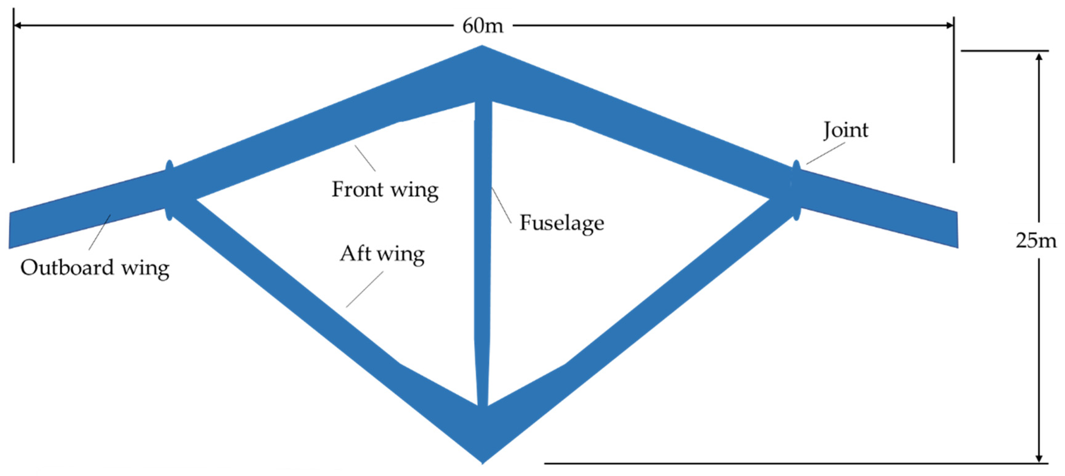
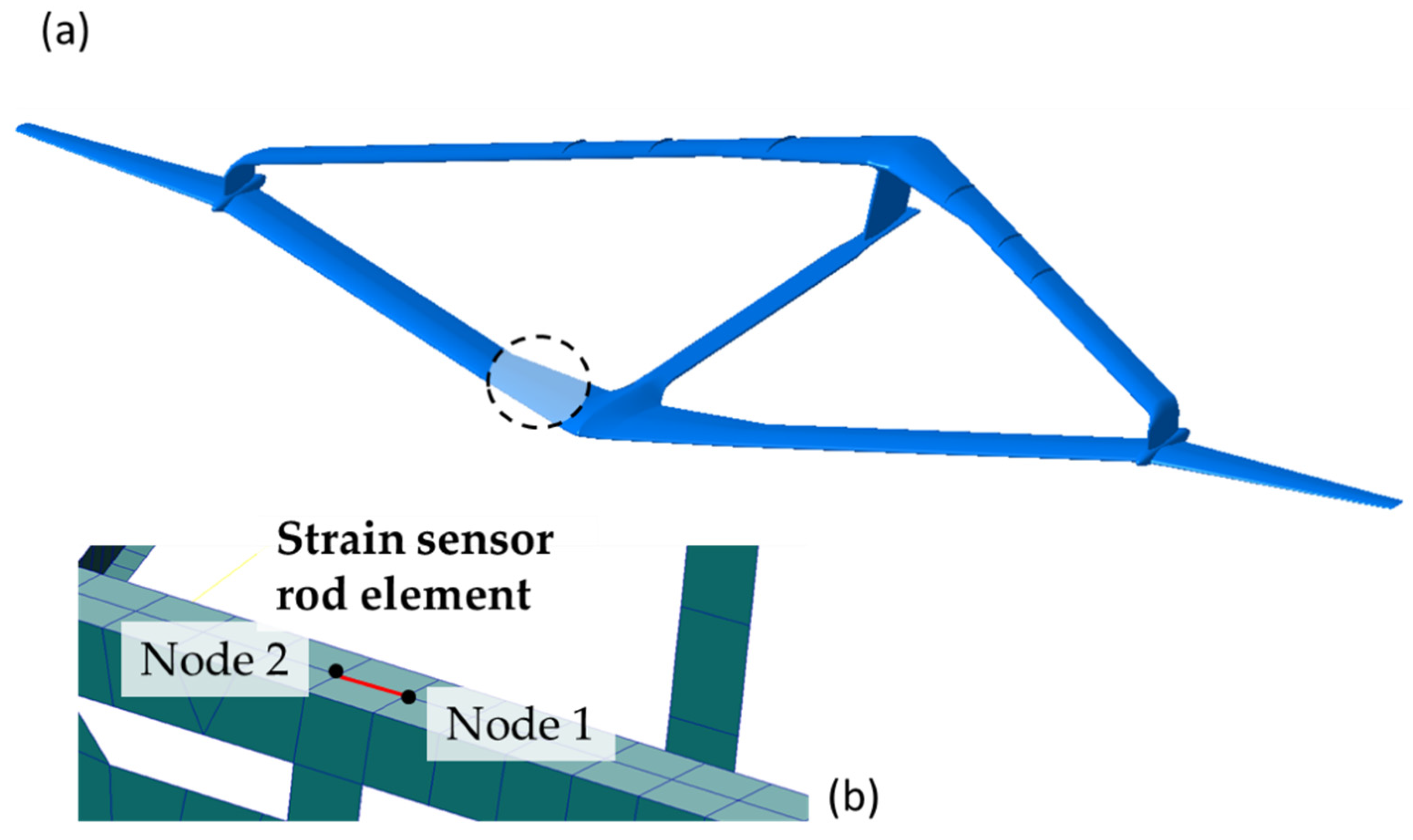
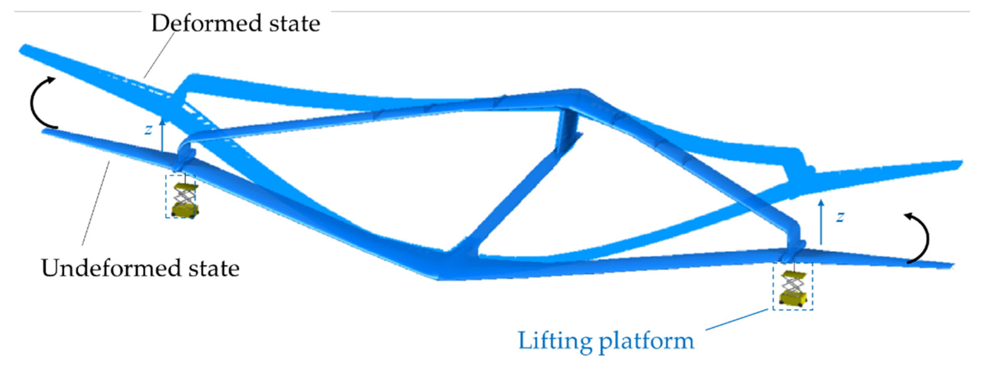
3.1. Model Description: A Joined-Wing Aircraft
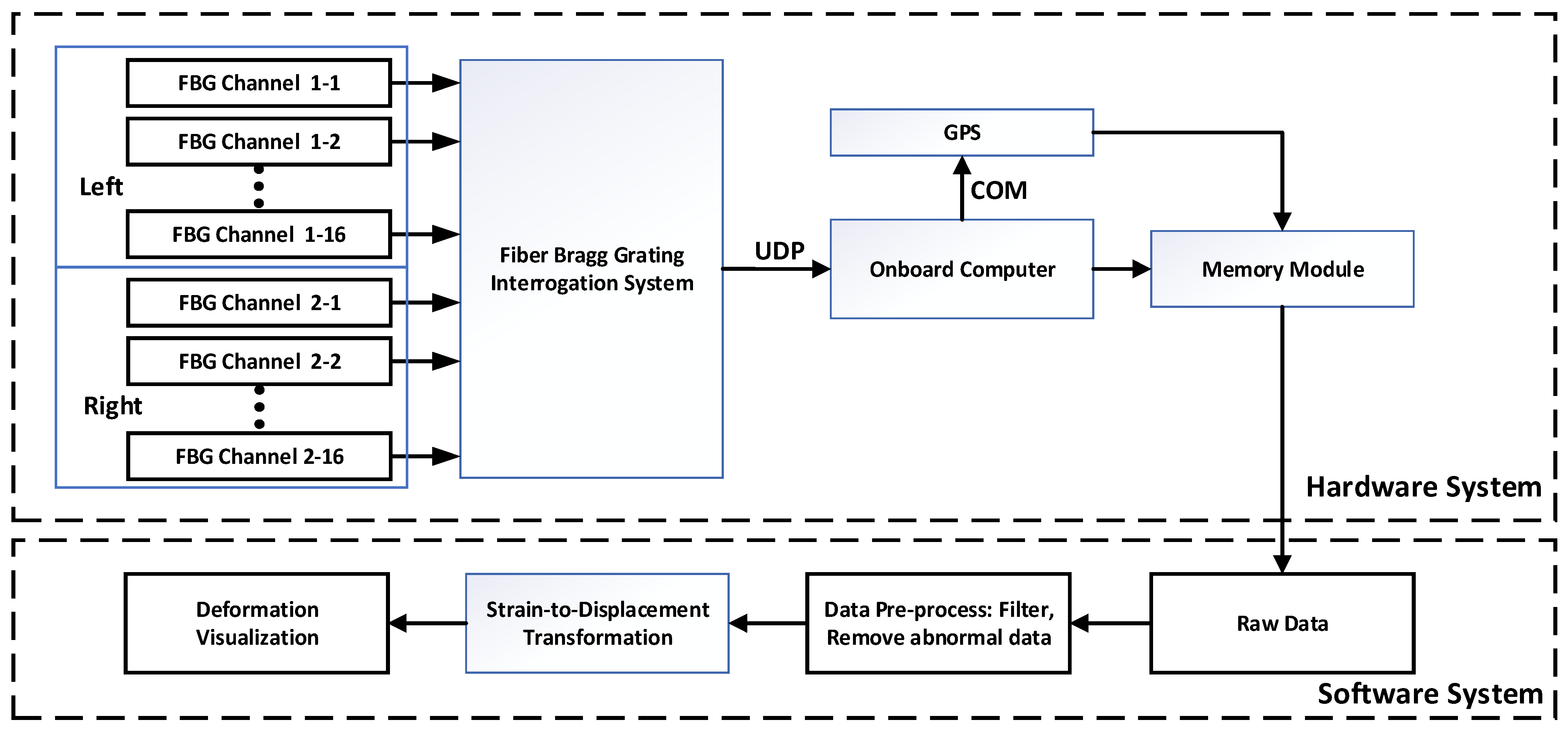
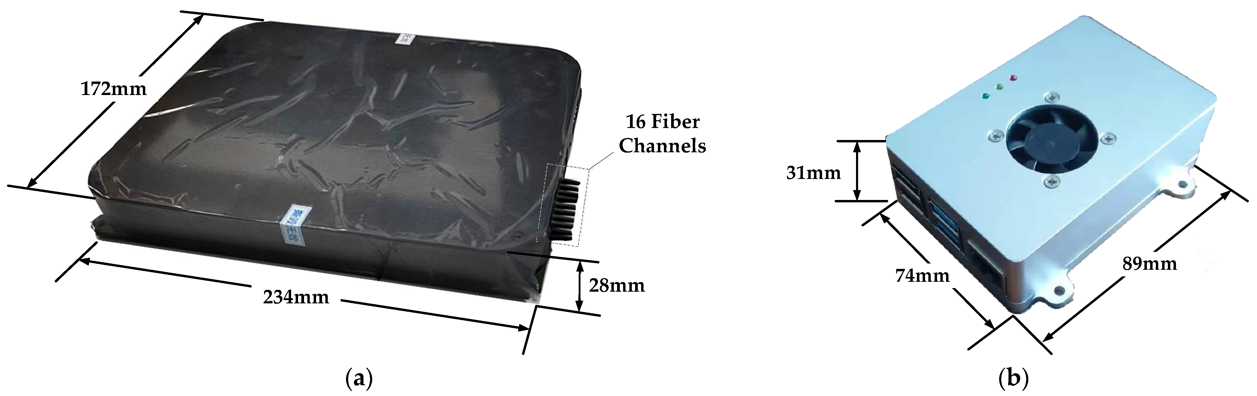
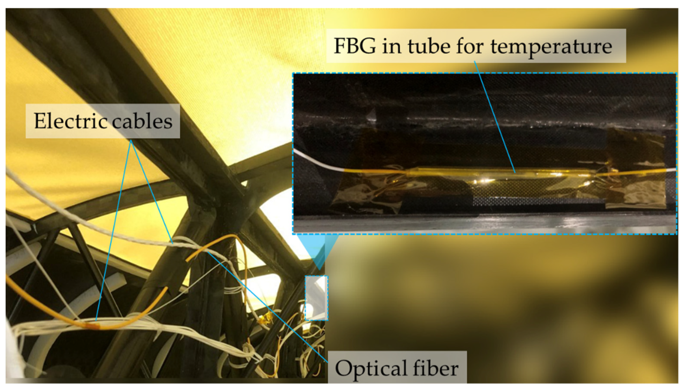
As shown in Figure 1, a Joined-Wing aircraft with diamond wings is designed and manufactured. The aircraft has a span length of approximately 60 m and a fuselage length of approximately 25 m. The main wing can be divided into front wing, aft wing and outboard wing. The front wing and the outboard wing are connected by two nacelles, which are further connected with the aft wing. The main structure of the aircraft is made of composite materials. The FOSS to be introduced next is mainly used to collect the strain information on the wing spar and predict the three-dimensional deformation of the entire wing.

3.2. FOSS Design

The overall scheme of the FOSS, including the hardware system and software system, is shown in Figure 2. The hardware system is divided into two independent systems for collecting and storing sensor data of the left and right wings. Each of the system consists of a FBG interrogation module, an onboard computer, a GPS and a memory module. The requirement of such an interrogation module would depend on the strain measurement along the front and aft wings of the 60-m wingspan. Figure 3a shows the interrogation system, the main parameters of which include an overall size of 234 mm × 172 mm × 28 mm, a sampling rate of 1000 Hz, 16 fiber channels, 1.04 kg weight and Ethernet interface. The environmental requirements were to meet a maximum wavelength shift of 5 pm under −10 °C to 50 °C operating temperature range, and a sine wave vibration in a range of 10–150 Hz with overload of 2 g. The characteristic wavelengths obtained by the interrogation system are transmitted to the onboard computer through UDP protocol. Meanwhile, the time series from GPS along with the fiber sensor data will be reorganized and stored in the memory module. The time consistency of test data from difference devices is guaranteed by the time series provided by GPS. Figure 3b shows the onboard computer, which has a 1.5 GHz 4-core CPU, a maximum RAM of 8 GB and multi-type interfaces including USB, HDMI, LAN, etc. The operating system is based on LINUX. A 64 GB Micro SD Card is used to store the sensor data. The onboard computer and a cooling fan are enclosed in an aluminum box with a size of 89 mm × 74 mm × 31 mm. The total weight is approximately 0.156 kg. Additionally, the main parameters of the used FBG sensor are listed in Table 1.
The software system was designed to transform the preprocessed sensing data into the structural deformation and display the final results. In general, the raw data are not directly used because of high-frequency noise and abnormal data. Therefore, the raw data need to be filtered, and the abnormal data need to be removed. After that, the desired structural deformations can be reconstructed by the STD transformation. Finally, the displacement response of arbitrary point on the structure or the whole structure configuration can be plotted by the visualization module.
In this work, the simplest and most effective filtering strategy was adopted, i.e., mean filtering. Denote the raw wavelength data as λ ( τ ) , then the filtered time series λ ( t ) can be expressed as:
λ ( t ) = 1 N t S λ ( τ )
in which S is the filter window with the size of N and the center at t . As mentioned before, interrogation system has a sampling rate of 1000 Hz, which is usually 5 Hz for GPS. By default, the window size N is set to 200.
The criterion for judging the abnormal data depends on the wavelength bandwidth and the strain range. The total wavelength bandwidth of a fiber channel is approximately 40 nm. To be specific, the interrogator is limited to identify Bragg wavelength within a range of 1529 nm to 1569 nm. The maximum number of FBGs multiplexed within an optic fiber is designed to be eight, which means the bandwidth occupied by one FBG sensor is at least 5nm. Therefore, the variation of the Bragg wavelength, δ λ B , is ±2.5 nm. Assuming the original Bragg wavelength λ B is approximately 1550 nm, the observed one can be (1550 ± 2.5) nm. According to Equation (2), the strain range can cover approximately ±2000 μ ε without consideration of temperature change. The strain range can basically meet the requirements of this work. Based on the above considerations, the wavelength variation exceeding 2.5 nm is considered as abnormal, i.e.,
| λ B λ B 0 | > 2.5
and needs to be removed.

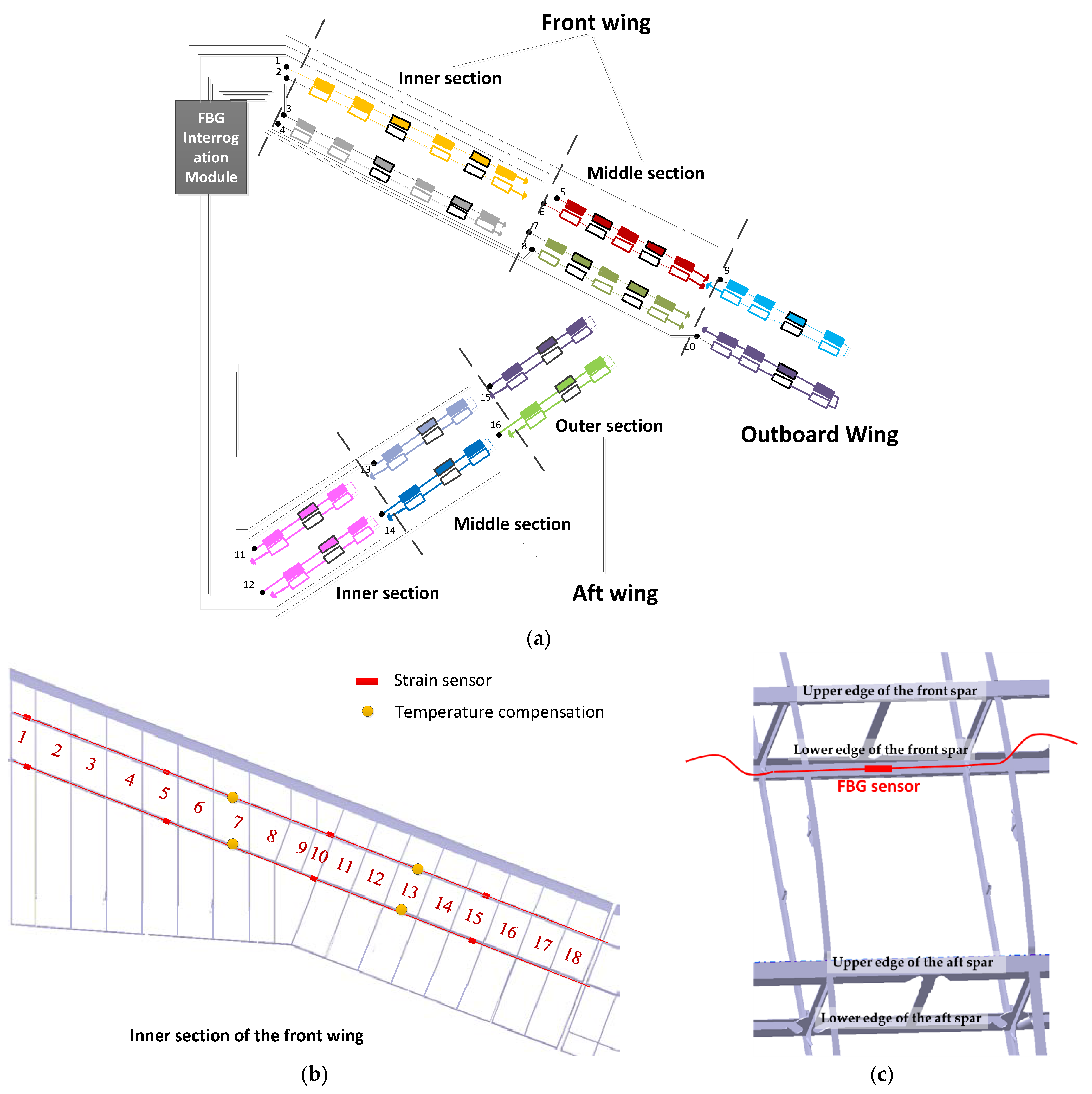
3.3. Sensor Arrangement

In this section, we will take the half model of the Joined-Wing aircraft as an example to illustrate the sensor layout and installation. Figure 4 shows the sensor layout of the right wing. As shown in Figure 4a, there are 16 fiber channels, each of which is multiplexed with different numbers of FBG sensors. For example, the optical fibers numbered 1–4 are used for strain and temperature measurements of the inner section of the front wing, as shown in Figure 4b. Each fiber contains six FBG sensors, which are represented by rectangular blocks, and the blocks with black border are used for temperature compensation. The solid ones are attached to the upper edge of the wing spar, while the hollow ones are attached to the lower edge. Figure 4c shows a detail view of FBG sensor installation on the surface of the spar. Due to the breakdown interfaces, the right wing is further divided into the six sections as shown in Figure 4a. The front wing and the aft wing consist of two sections and three sections, respectively.
Figure 5 is a snapshot of the wing interior. Both the electric cables and the optical fibers are bundled with the skeleton inside the wing. The FBG sensors are attached to the spar surfaces using epoxy adhesive. The temperature compensation is realized by the FBG sensor in a tube with a rigid steel needle inside.

4. Results and Discussion

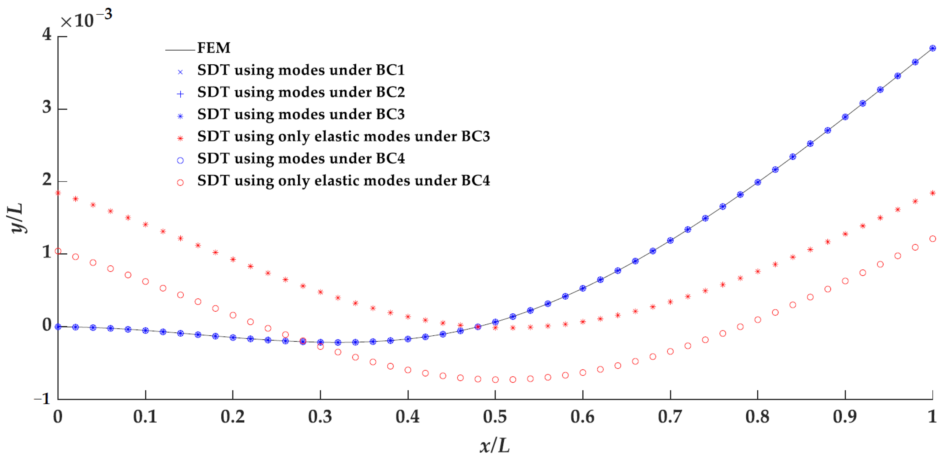
4.1. Validation on a Cantilever Beam Model

A cantilever beam supported at the midpoint was first investigated to demonstrate the improved modal method. The beam has a rectangular cross-section with a width of 0.035 m and a height of 0.0015 m. The elastic modulus is 210 GPa. The material density is 7750 kg/m3. As shown in Figure 6, a concentrated force is applied at the beam tip, with its vertical components being 0.1 N. The beam is solved in MSC NASTRAN with the discretization of 50 elements.
Four types of boundary conditions are considered for linear modal analysis. The first one is consistent with Figure 6, in which the beam is fixed at the root and supported at the midpoint. The second and third ones retain fixed and supported constraints, respectively. The fourth one is totally free without any constraint. The mathematical expressions of the boundary conditions are given in Equation (16).
{ BC 1 : y ( 0 ) = y ( 0 ) = 0 , y ( L / 2 ) = 0 BC 2 : y ( 0 ) = y ( 0 ) = 0 BC 3 : y ( L / 2 ) = 0 BC 4 : f r e e f r e e
Mode shapes obtained through the modal analysis can be found in Appendix A. As expected, a rigid-body rotational mode around the support point occurs in the third case. In the last case, one may find an axial mode and two rigid-body modes, which are superpositions of y-direction motion and rotational motion around z-axis.
Figure 7 presents the comparisons of displacement directly computed from FEM and those obtained from SDT under different conditions. In all cases, the first 20 modes with no distinction between rigid-body modes and elastic modes are used for SDT. Under BC1 and BC2, the displacements are computed by Equation (7) consistent with the classical modal approach. Under BC3 and BC4, the displacements are computed by the improved modal method due to the existence of rigid-body modes. Additionally, the predicted displacements show differences when only elastic modes are considered under BC3 and BC4. The differences are perfectly compensated by superposition of rigid-body motions. Finally, one can observe that the predicted displacements are highly consistent with the FEM results, no matter what boundary conditions are adopted.

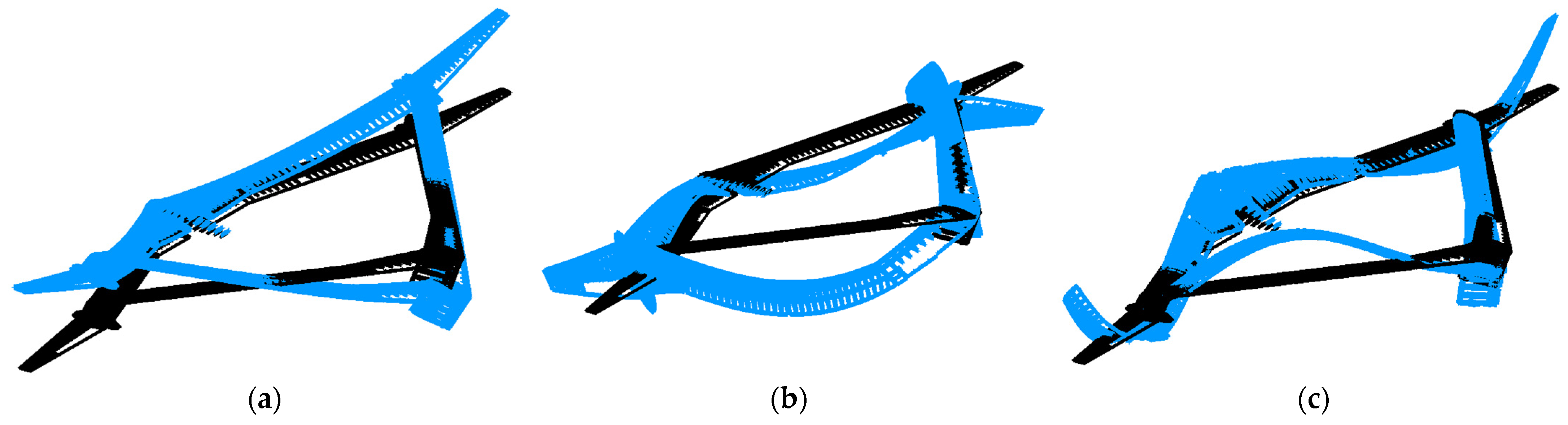
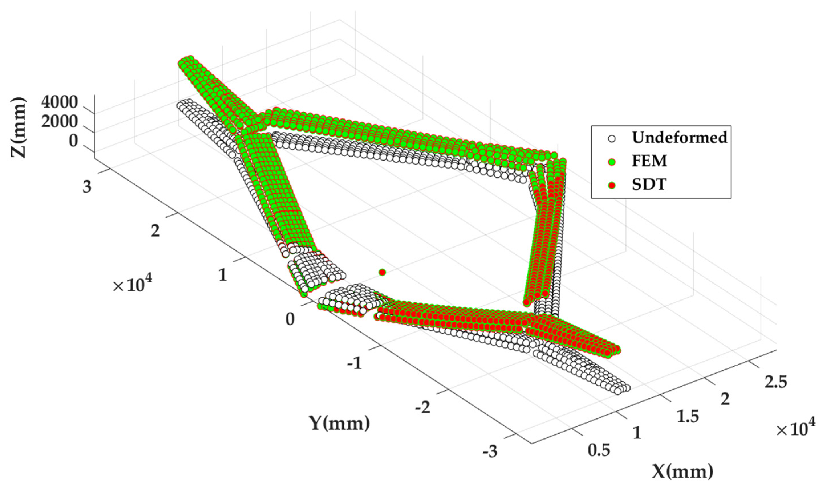
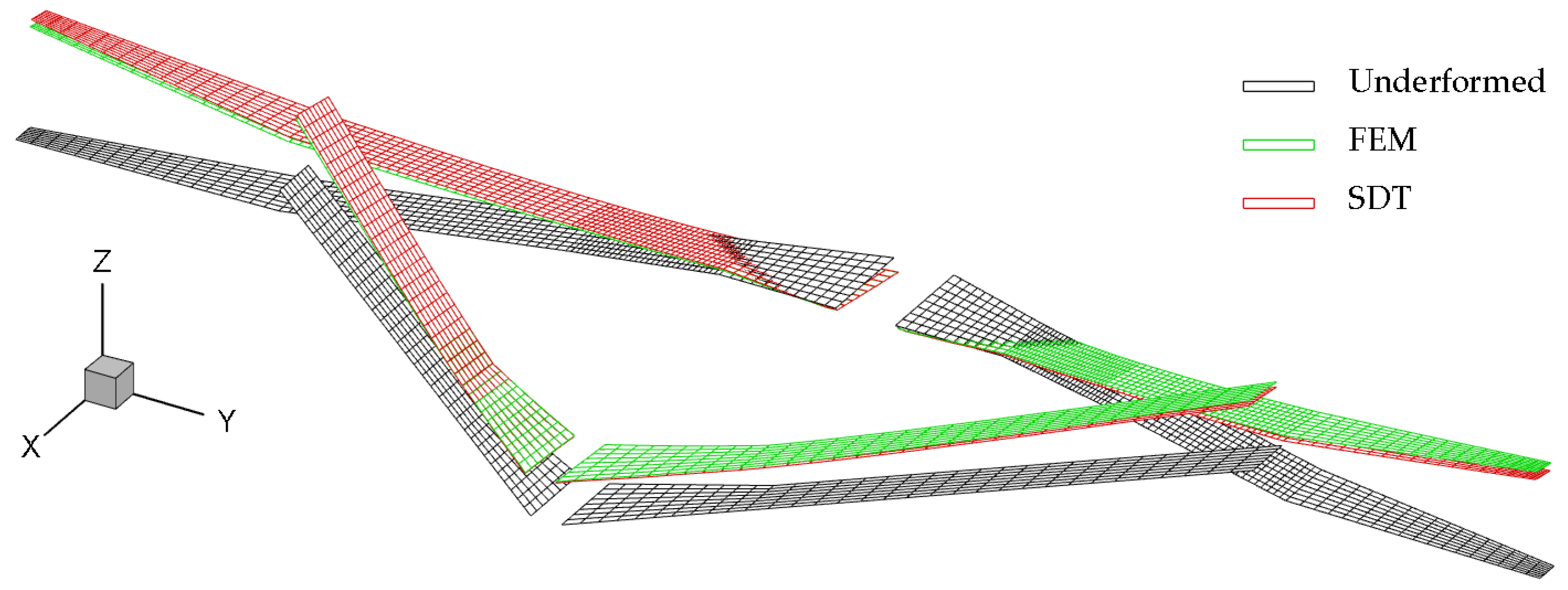
4.2. Numerical Studies on the Joined-Wing Aircraft

The FE model was constructed from the original CAD model in MSC NASTRAN, as shown in Figure 8a. Most of the structures including the wing spars and skin were modeled using composite plate elements. The fuselage skeleton uses a large number of bar elements. The FE model has approximately 370,000 nodes and 340,000 elements. A number of 64 massless rod elements with negligible stiffness were attached to the spar surface of both right and left wing, respectively. These elements do not change the stiffness and inertial properties of the original aircraft model. They are distributed at the positions in accordance with the sensor layout in Figure 4, serving as virtual strain sensors to provide strain information at these locations. Figure 8b shows a schematic view of a rod element.
Modal analysis was then conducted to obtain mode frequencies and mode shapes of both displacement modes and strain modes. The strain modes are provided by the virtual strain sensor elements. The boundary condition is set to free–free without constraints. The first 30 modes are used for SDT. The first six modes are rigid-body modes. Several primary elastic mode shapes are plotted in Figure 9. The first symmetric vertical bending mode has a very low frequency of 0.354 Hz. Different from the common-configuration aircraft, a distinctive modal feature of the joined-wing configuration is the coupling of the front wing and the aft wing, which can be found in Figure 9b,c.
In the linear static solver of MSC NASTRAN, the six degrees of freedom (DOFs) of the grid point coincident with the mass center are constrained. One times gravity loads along the anti-gravity direction are applied to make the wing bend upward. The free–free modes were used for SDT. Figure 10 shows the comparison of an undeformed and deformed configuration under such loading conditions. The displacements calculated directly by FEM are in very good agreement with those reconstructed by SDT. The maximum displacement in z-axis direction is up to 4.71 m, which is approximately 14.1% of the half wingspan. Due to the complexity of the FE model with up to two million DOFs, it is too time-consuming to reconstruct the deformation using the modal information of all nodes. Here, we select 1188 grid points on the wing structure for SDT. Three rotational DOFs in the displacement modal vector are ignored. In this way, the matrix of displacement mode Φ in Equation (4) has 3564 rows and 30 columns. The matrix of strain mode φ in Equation (5) has 196 rows and 30 columns. Although only the deformation of the selected grid points is shown here, the position of any other point inside the whole aircraft can be conveniently calculated by surface spline interpolation [29]. Figure 11 presents the interpolated lifting surface, which is used to conveniently and efficiently evaluate the overall deformation of the aircraft.
To quantitatively investigate the deformation reconstruction accuracy, the following two kinds of Root Mean Square Errors (RMSE) are used,
R M S E 1 = i = 1 N ( z i z ^ i ) 2 / i = 1 N z i 2
R M S E 2 = ( z i max z ^ i max ) 2 / z i max 2
In Equation (17), z is the displacement in z-axis direction calculated by FEM, and z ^ is the displacement calculated by SDT. The subscript i is the index number of the grid point, and N is the total number of grid points. In Equation (18), i max represents the node number with the maximum displacement. These two equations provide a global and local evaluation of deformation reconstruction accuracy, respectively. Finally, the global error R M S E 1 is 2.86%, and the local error R M S E 2 is 4.47%. The results further show the accuracy of SDT in reconstructing the wing deformation.

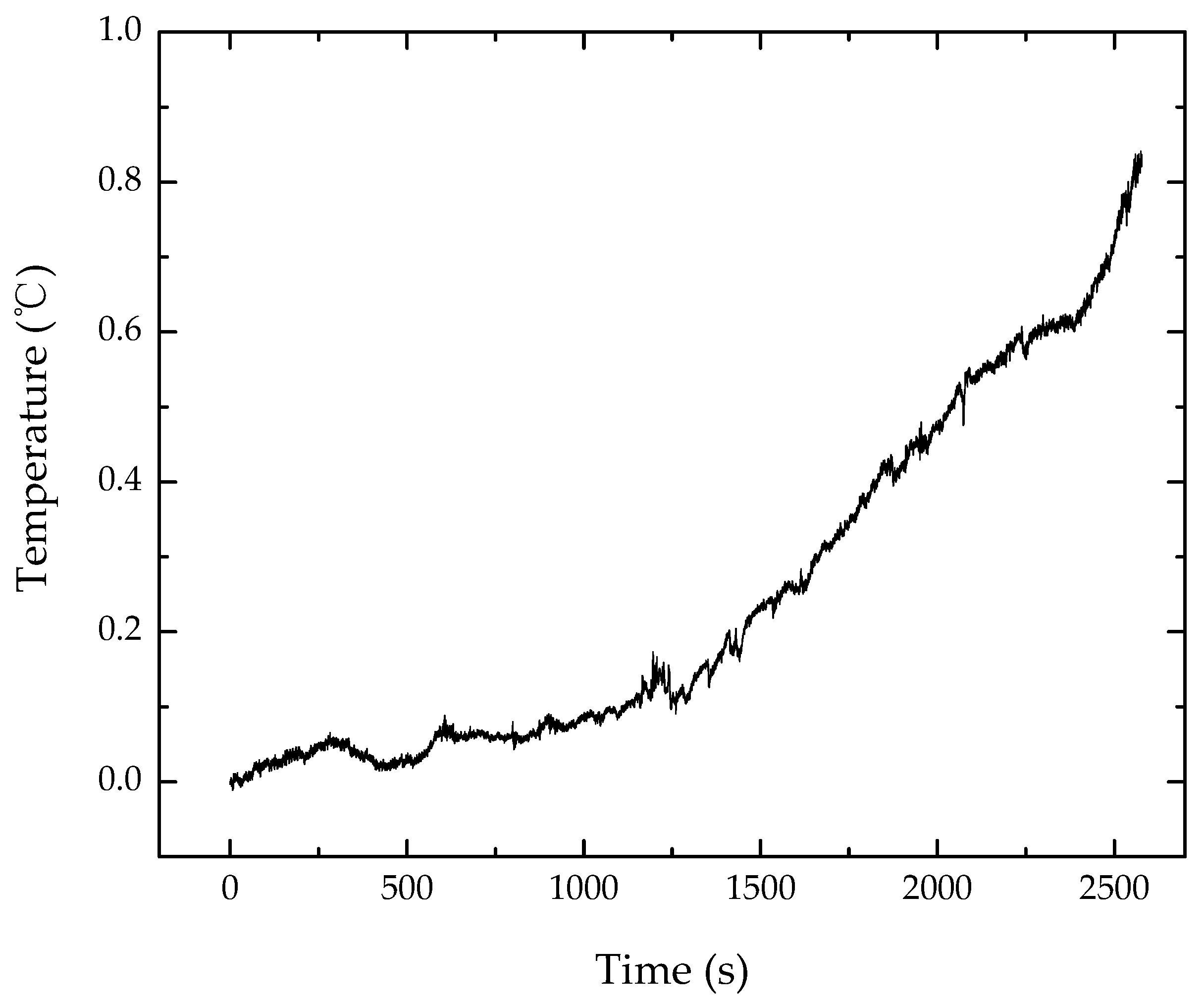
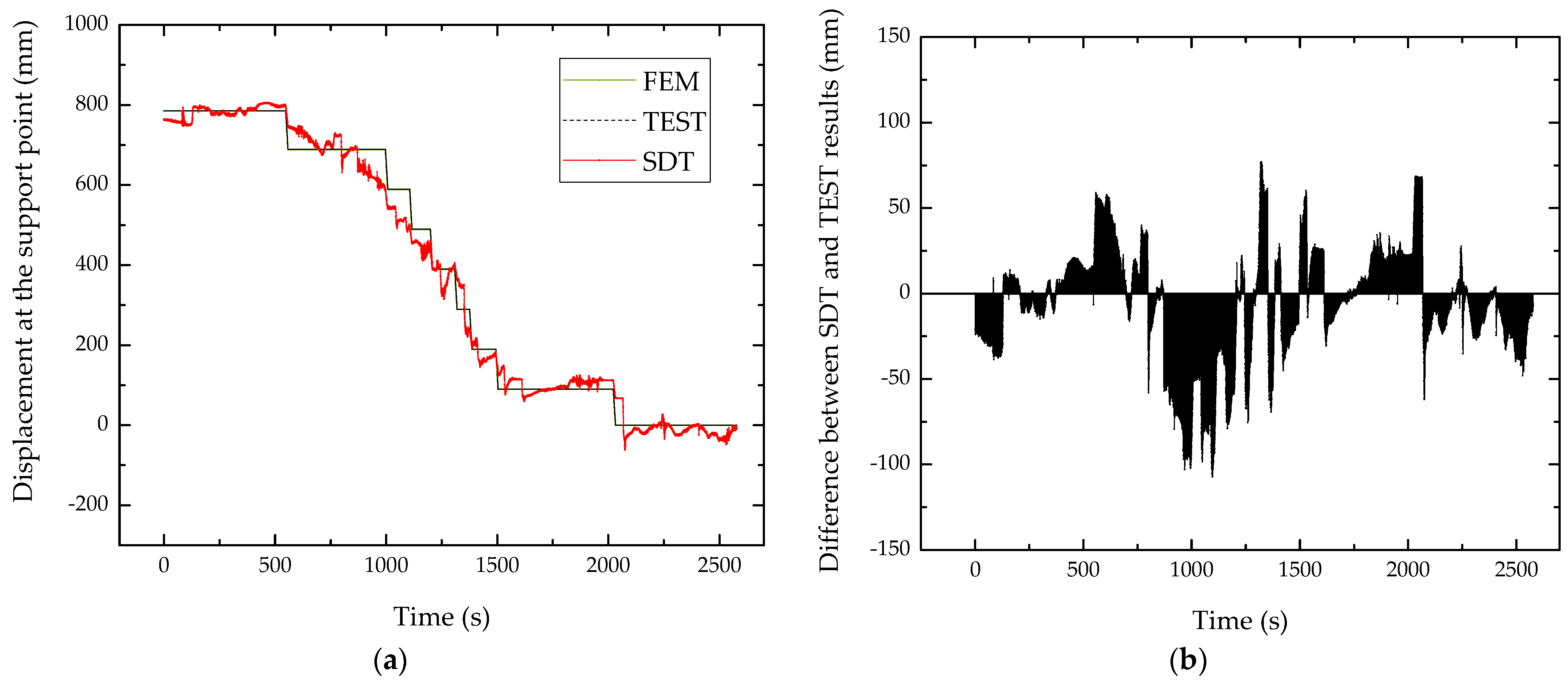
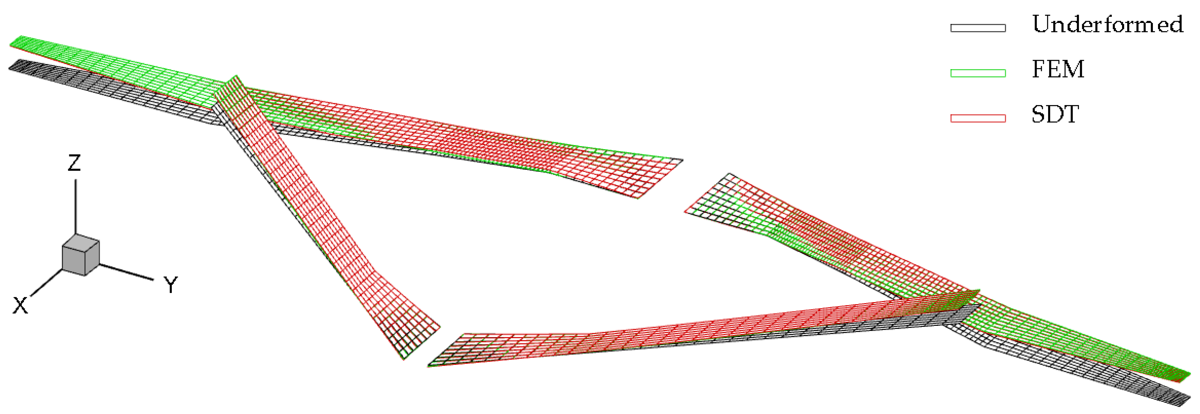
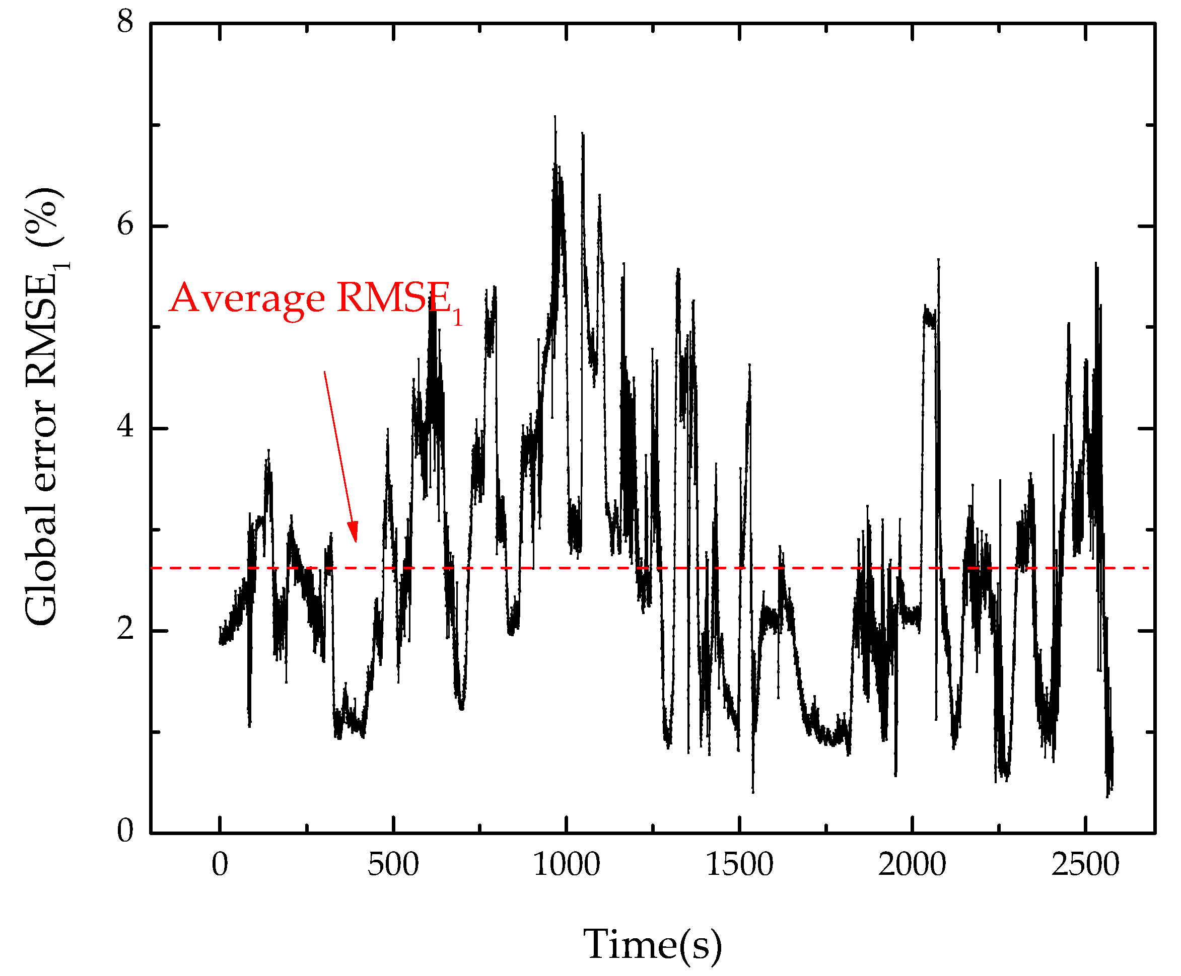
4.3. Ground Test on the Joined-Wing Aircraft

The system’s performance was then evaluated in a ground quasi-static test in which the wing was lifted by two lifting platforms under the nacelles at the joint. Figure 12 shows the schematic of the ground test. The lifting attitude z can be accurately controlled by the lifting platform. Before the test, the Joined-Wing aircraft was on the ground supported by two front main landing gears, two auxiliary landing gears and a rear landing gear. The optical fiber sensing data in this state were recorded as the initial reference value. At the beginning of the test, the lifting attitudes of both right and left side were set to 785 mm. After holding on for a certain time, the lifting altitude may drop by approximately 100 mm within approximately 10 s. The above maintenance and decent operations will be repeated several times until the altitude drops to zero, which means the aircraft returns to its initial reference state. Table 2 lists the lifting altitudes over time and the specific operations, which are recorded as H and D (Hold and Drop). The ground test lasted nearly 2000 s. The altitudes were reduced from 785 mm to 0 mm in 7 operations.
Figure 13 plots the temperature curve recorded by FBG sensors. Since the test is in a relatively closed indoor environment, we assume that the temperature is independent of the location. Therefore, the temperature curve reflects the average of collected data from all FBG sensors for temperature compensation. According to the records of the onboard temperature sensor with limited precision, the temperature increased from 22 °C to 23 °C during the test. The test was conducted from 2:00 pm to 3:00 pm, during which time the temperature rose slowly. The results of temperature sensor and FBG sensor show that the temperature change during the test is less than 1 °C, which means the temperature effect on the following strain data acquisition is almost negligible.
Figure 14a plots the displacement responses at the support point during the ground test. The deformations on both sides of the wing are approximately considered symmetrical, specifically synchronous and of the same size. Thus, the displacement plotted in this figure is the average of the z-direction deformation at the left and right support points. The test results are consistent with those listed in Table 2. As a comparison, wing displacements were also obtained from FEM. To simulate the ground test, we constrained the translational DOFs of four nodes at the front of fuselage and one node at the rear of the fuselage. These nodes are consistent with the positions of landing gears. As for the nodes corresponding to the support point, translational DOFs except the vertical motion are constrained. Nodal forces are applied to the support point towards positive z-direction to simulate the deformation during the test. The results show that the numerical simulation accurately reflects the displacement response in the test. The difference between SDT and TEST results is plotted in Figure 14b. The absolute displacement error is within ±100 mm. One can also calculate the relative error in the manner similar to Equation (17) by replacing i and N with time variables corresponding to the horizontal axis in the figure. The calculated error is 6.6%. The error mainly comes from two aspects. One is the model-related error. For such a complex engineering model, the deviation between the FE model and the realistic one is inevitable. Additionally, the sensor placement and the mode selection will affect the reconstruction accuracy. Future efforts can be made to improve the accuracy by optimizing the sensor positions and selected mode as in Ref. [22]. The second one is the test-related error. In the test, the strain measured by the FBG sensor is affected by the adhesive layer and cannot exactly reflect the strain on the structural surface. It is challenging to analyze and predict the strain transfer to the fiber core reliably, which is beyond the scope of this work. A practical way is to consider the error caused by strain transfer as uncertainties satisfying normal distribution, and then to achieve more reliable results by filtering methods.
Figure 15 shows the deformed configuration obtained from FEM and SDT at the beginning of the test. The overall deformation obtained by direct numerical simulation is in good agreement with that reconstructed by measured strains. Taking FEM results as reference, the global error RMSE1 at each moment was calculated and plotted in Figure 16. The maximum error is approximately 7%. The average error is 2.62%. The results show that the FOSS and SDT algorithm in this work can accurately measure the deformation of the Joined-Wing aircraft during the ground test.

5. Conclusions

This work presents a complete framework for predicting structural displacement of a Joined-Wing aircraft by using Fiber Optic Sensing techniques. Several concluding remarks can be drawn as follows:
(1)
A FOSS with hardware and software subsystems is designed and installed on the target Joined-Wing aircraft. The system was then verified by the ground test.
(2)
The classical modal method is modified to adapt to various boundary conditions, which is common in practical applications. The improved SDT algorithm was then verified by numerical studies on a cantilever beam model and the Joined-Wing aircraft.
(3)
Both the numerical and experimental results show that the proposed SDT algorithm can accurately predict the overall configuration of the aircraft or deformations of a particular point. In the ground test, the relative error of the displacement at the support point is 6.6%. The global error of the overall deformation is less than 7%, and the average error is only 2.62%.
In general, the FOSS was proved to have reasonable accuracy and the potential for future flight tests.

Author Contributions

Conceptualization, Y.M. and C.X.; Data curation, Y.B.; Methodology, Y.M. and Z.C.; Software, Y.M.; Supervision, C.Y.; Validation, Y.B. and C.X.; Writing—original draft, Y.M.; Writing—review and editing, Y.B. and C.X. All authors have read and agreed to the published version of the manuscript.

Funding

This research received no external funding.

Data Availability Statement

Not applicable.

Acknowledgments

We would appreciate Ziqiang Wang for his support in hardware system development and ground test.

Conflicts of Interest

The authors declare no conflict of interest.

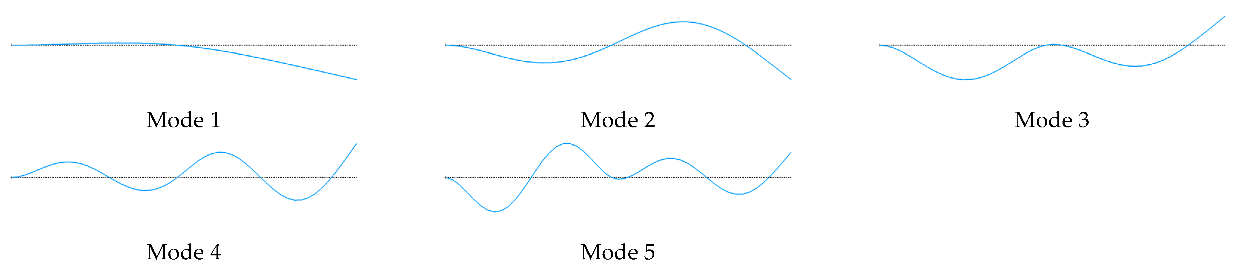
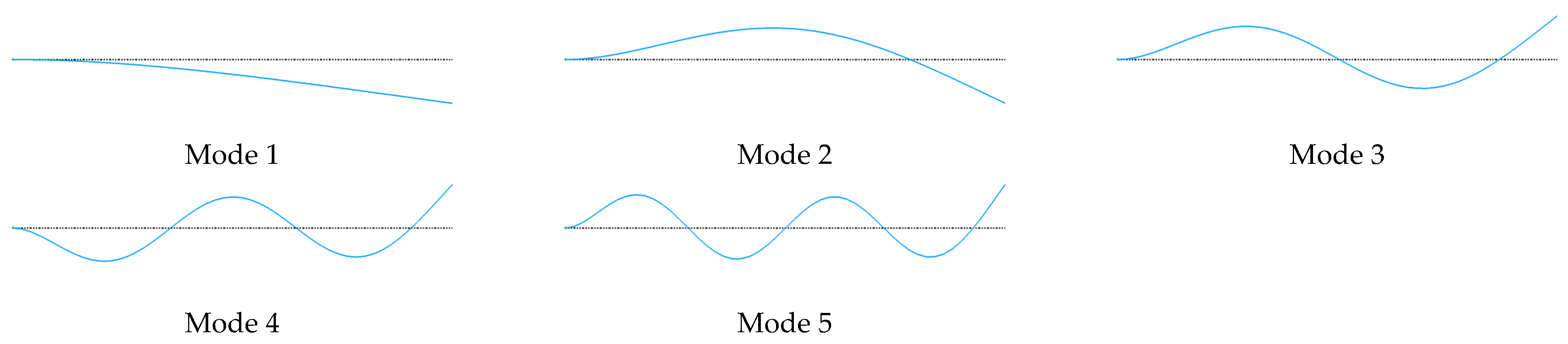
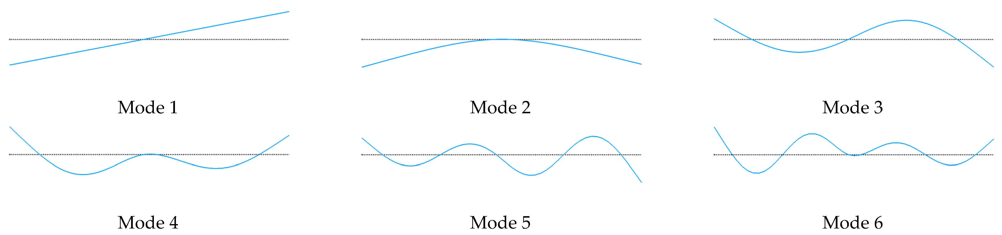
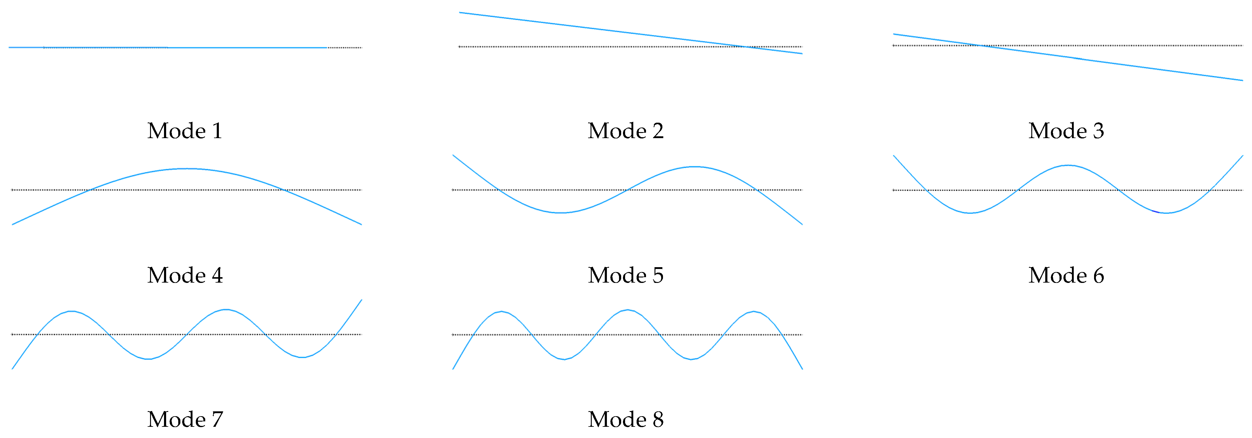
Appendix A. Mode Shapes of the Cantilever Beam Model with Different Boundary Conditions

Figure A1. First five elastic modes with BC1: y ( 0 ) = y ( 0 ) = y ( L / 2 ) = 0 .
Aerospace 09 00661 g0a1
Figure A2. First five elastic modes with BC2: y ( 0 ) = y ( 0 ) = 0 .
Aerospace 09 00661 g0a2
Figure A3. Rigid-body mode and first five elastic modes with BC3: y ( L / 2 ) = 0 .
Aerospace 09 00661 g0a3
Figure A4. Rigid-body modes and first five elastic modes with BC4: free–free.
Aerospace 09 00661 g0a4

References

  1. Cavallaro, R.; Demasi, L. Challenges, Ideas, and Innovations of Joined-Wing Configurations: A Concept from the Past, an Opportunity for the Future. Prog. Aerosp. Sci. 2016, 87, 1–93. [Google Scholar] [CrossRef]
  2. Tilmann, C.P.; Flick, P.M.; Martin, C.A.; Love, M.H. High-Altitude Long Endurance Technologies for SensorCraft. In Proceedings of the RTO Paper MP-104-P-26, RTO AVT Symposium on Novel and Emerging Vehicle and Vehicle Technology Concepts, Brussels, Belgium, 7–11 April 2003. [Google Scholar]
  3. Su, W. Coupled Nonlinear Aeroelasticity and Flight Dynamics of Fully Flexible Aircraft; University of Michigan: Ann Arbor, MI, USA, 2008. [Google Scholar]
  4. Cavallaro, R.; Iannelli, A.; Demasi, L.; Razon, A.M. Phenomenology of nonlinear aeroelastic responses of highly deformable joined wings. Adv. Aircr. Spacecr. Sci. 2015, 2, 125–168. [Google Scholar] [CrossRef]
  5. Ma, Z.; Chen, X. Fiber Bragg Gratings Sensors for Aircraft Wing Shape Measurement: Recent Applications and Technical Analysis. Sensors 2018, 19, 55. [Google Scholar] [CrossRef] [PubMed] [Green Version]
  6. Floris, I.; Adam, J.M.; Calderón, P.A.; Sales, S. Fiber Optic Shape Sensors: A comprehensive review. Opt. Lasers Eng. 2021, 139, 106508. [Google Scholar] [CrossRef]
  7. Masoudi, A.; Newson, T.P. Contributed Review: Distributed optical fibre dynamic strain sensing. Rev. Sci. Instrum. 2016, 87, 011501. [Google Scholar] [CrossRef] [PubMed] [Green Version]
  8. Noll, T.E.; Brown, J.M.; Perez-Davis, M.E.; Ishmael, S.D.; Tiffany, G.C.; Gaier, M. Investigation of the Helios Prototype Aircraft Mishap; Volume I Mishap Report; NASA: Washington, DC, USA, 2004. [Google Scholar]
  9. Ko, W.L.; Richards, W.L.; Tran, V.T. Displacement Theories for In-Flight Deformed Shape Predictions of Aerospace Structures; NASA Dryden Flight Research Center: Edwards, CA, USA, 2007. [Google Scholar]
  10. Ko, W.L.; Fleischer, V.T. Further Development of Ko Displacement Theory for Deformed Shape Predictions of Nonuniform Aerospace Structures; NASA Dryden Flight Research Center: Edwards, CA, USA, 2009. [Google Scholar]
  11. Derkevorkian, A.; Masri, S.F.; Alvarenga, J.; Boussalis, H.; Bakalyar, J.; Richards, W.L. Strain-Based Deformation Shape-Estimation Algorithm for Control and Monitoring Applications. AIAA J. 2013, 51, 2231–2240. [Google Scholar] [CrossRef]
  12. KO, W.L.; Richards, W.L.; Fleischer, V.T. Applications of KO Displacement Theory to the Deformed Shape Predictions of the Doubly-Tapered Ikhana Wing; NASA Dryden Flight Research Center: Edwards, CA, USA, 2009. [Google Scholar]
  13. Nicolas, M.J.; Sullivan, R.W.; Richards, W.L. Large Scale Applications Using FBG Sensors: Determination of In-Flight Loads and Shape of a Composite Aircraft Wing. Aerospace 2016, 3, 18. [Google Scholar] [CrossRef] [Green Version]
  14. Klotz, T.; Pothier, R.; Walch, D.; Colombo, T. Prediction of the business jet Global 7500 wing deformed shape using fiber Bragg gratings and neural network. Results Eng. 2020, 9, 100190. [Google Scholar] [CrossRef]
  15. Meng, Y.; Xie, C.C.; Wan, Z.Q. Deformed Wing Shape Prediction using Fiber Optic Strain Data. In Proceedings of the International Forum on Aeroelasticity and Structural Dynamics, Como, Italy, 25–28 June 2017. [Google Scholar]
  16. Tessler, A.; Spangler, J.L. A least-squares variational method for full-field reconstruction of elastic deformations in shear-deformable plates and shells. Comput. Methods Appl. Mech. Eng. 2005, 194, 327–339. [Google Scholar] [CrossRef]
  17. Tessler, A. Structural Health Monitoring Using High-Density Fiber Optic Strain Sensor and Inverse Finite Element Methods; NASA Langley Research Center TM-214871: Hampton, VA, USA, 2007. [Google Scholar]
  18. Gherlone, M.; Cerracchio, P.; Mattone, M.; Di Sciuva, M.; Tessler, A. Shape sensing of 3D frame structures using an inverse Finite Element Method. Int. J. Solids Struct. 2012, 49, 3100–3112. [Google Scholar] [CrossRef]
  19. Gherlone, M.; Cerracchio, P.; Mattone, M.; Di Sciuva, M.; Tessler, A. An inverse finite element method for beam shape sensing: Theoretical framework and experimental validation. Smart Mater. Struct. 2014, 23, 045027. [Google Scholar] [CrossRef] [Green Version]
  20. Tessler, A.; Roy, R.; Esposito, M.; Surace, C.; Gherlone, M. Shape Sensing of Plate and Shell Structures Undergoing Large Displacements Using the Inverse Finite Element Method. Shock Vib. 2018, 2018, 8076085. [Google Scholar] [CrossRef]
  21. Gherlone, M.; Cerracchio, P.; Mattone, M. Shape sensing methods: Review and experimental comparison on a wing-shaped plate. Prog. Aerosp. Sci. 2018, 99, 14–26. [Google Scholar] [CrossRef]
  22. Esposito, M.; Gherlone, M. Composite wing box deformed-shape reconstruction based on measured strains: Optimization and comparison of existing approaches. Aerosp. Sci. Technol. 2020, 99, 105758. [Google Scholar] [CrossRef]
  23. Foss, G.C.; Haugse, E.D. Using Modal Test Results to Develop Strain to Displacement Transformations. In SPIE The International Society for Optical Engineering; SPIE: Bellingham, WA, USA, 1995; p. 112. [Google Scholar]
  24. A Davis, M.; Kersey, A.D.; Sirkis, J.S.; Friebele, E.J. Shape and vibration mode sensing using a fiber optic Bragg grating array. Smart Mater. Struct. 1996, 5, 759–765. [Google Scholar] [CrossRef]
  25. Kang, L.-H.; Kim, D.-K.; Han, J.-H. Estimation of dynamic structural displacements using fiber Bragg grating strain sensors. J. Sound Vib. 2007, 305, 534–542. [Google Scholar] [CrossRef]
  26. Kim, H.; Han, J.; Bang, H. Real-time deformed shape estimation of a wind turbine blade using distributed fiber Bragg grating sensors. Wind. Energy 2014, 17, 1455–1467. [Google Scholar] [CrossRef]
  27. Freydin, M.; Rattner, M.K.; Raveh, D.E.; Kressel, I.; Davidi, R.; Tur, M. Fiber-Optics-Based Aeroelastic Shape Sensing. AIAA J. 2019, 57, 5094–5103. [Google Scholar] [CrossRef]
  28. Martins, B.L.; Kosmatka, J.B. Health Monitoring of Aerospace Structures via Dynamic Strain Measurements: An Experimental Demonstration. In Proceedings of the AIAA Scitech 2020 Forum, Orlando, FL, USA, 6–10 January 2020. [Google Scholar] [CrossRef]
  29. Chang, C.X.; Chao, Y.; Xie, C.; Yang, C. Surface Splines Generalization and Large Deflection Interpolation. J. Aircr. 2007, 44, 1024–1026. [Google Scholar] [CrossRef]
Figure 1. Top view of the Joined-Wing aircraft.
Aerospace 09 00661 g001
Figure 2. Overall design of FOSS.
Aerospace 09 00661 g002
Figure 3. (a) FBG Interrogation System; (b) onboard computer.
Aerospace 09 00661 g003
Figure 4. Sensor layout. (a) The overall sensor arrangement of the half model; (b) sensor arrangement of the inner section of the front wing; (c) detail view of FBG sensor installation on the surface of the spar.
Aerospace 09 00661 g004
Figure 5. Wing interior and sensor attachment on the wing spar.
Aerospace 09 00661 g005
Figure 6. Cantilever beam model with a tip force.
Aerospace 09 00661 g006
Figure 7. Comparisons of calculated displacements from FEM and those obtained from SDT.
Aerospace 09 00661 g007
Figure 8. (a) FE model and (b) zoom on the front spar of the front wing and a rod element to simulate strain sensor.
Aerospace 09 00661 g008
Figure 9. Several primary elastic mode shapes: (a) 7th mode—symmetric vertical bending, f 1 = 0.354   Hz ; (b) 13th mode—anti-symmetric vertical bending coupled with torsion, f 7 = 1.101   Hz ; (c) 30th mode—symmetric vertical bending coupled with torsion, f 30 = 3.234   Hz .
Aerospace 09 00661 g009
Figure 10. Positions of selected grid points in undeformed configuration and deformed configuration under gravity loads along the anti-gravity direction.
Aerospace 09 00661 g010
Figure 11. Interpolated lifting surfaces for evaluation of overall deformation.
Aerospace 09 00661 g011
Figure 12. A schematic of ground test.
Aerospace 09 00661 g012
Figure 13. Temperature during the ground test recorded by FBG sensors.
Aerospace 09 00661 g013
Figure 14. (a) Displacement responses at the support point; (b) difference between SDT and TEST results.
Aerospace 09 00661 g014
Figure 15. Deformed configuration obtained from FEM and SDT at the beginning of the test.
Aerospace 09 00661 g015
Figure 16. Global error response of SDT.
Aerospace 09 00661 g016
Table 1. The main parameters of FBG sensor.
ParameterValue
3 dB bandwidth≤0.3 nm
Reflectivity≥90%
Side Lobe Suppression (SLS)≥15 dB
Grating length10 mm
Temperature sensitivity (temperature-optic coefficient)6.67 K−1·10−6
Strain sensitivity (strain-optic coefficient)7.8 με−1·10−7
Table 2. Lifting altitudes of the lifting platform and operations at different time.
Time (s) Lifting   Altitude   z Operation (H-Hold/D-Drop)
0785H
265785D
275690H
375690D
385590H
468590D
478490H
578490D
588390H
645390D
655290H
763290D
773190H
1294190D
130490H
185490D
18640H
Publisher’s Note: MDPI stays neutral with regard to jurisdictional claims in published maps and institutional affiliations.

