Multi-Scale Mechanical Property Prediction for Laser Metal Deposition

Abstract

The Laser Metal Deposition (LMD) involves extremely complex multi-scale multi-physics and multiple thermal cycles issues, making it difficult to accurately predict the resultant mechanical properties of fabricated components from given process parameters. This research, by proposing a cladding stacking model that uses the structural evolution history of the heat-affected zone, predicts the overall structure of fabricated components, and establishes a process–structure–property multi-scale simulation framework based on this model, a general solution for the abovementioned difficulty. Based on the Hot Optimal Transportation Meshfree (HOTM) method, a platform ESCAAS is developed to simulate the meso-scale Ti-6Al-4V powder evolution process. Based on the Cellular Automaton (CA) method, the micro-scale grain structure in the molten pool is simulated. The macro-scale mechanical property of the fabricated component is calculated based on a polycrystalline Representative Volume Element (RVE) model and the homogenization technology. Experiments including LMD multilayer printings, metallographic observations, and static tension are designed to verify the accuracy of the model and simulations. The results are greatly consistent with the experimental data and the relative error of the final mechanical property prediction is within 5.18%. This work provides a basis for the quantitative analysis of the process–structure–property relationship and the optimization of process parameters.

1. Introduction

The increasing structural complexity of aerospace components has brought great difficulties to the traditional manufacturing processes. The Laser Metal Deposition (LMD) process based on the coaxial powder feeding, through the interaction of metal powders and lasers, makes the powders quickly melt and accumulate layer by layer, brings great convenience to the manufacture of complex components and has attracted much attention in the aerospace field [1,2]. Wang [3] fabricated large critical load-carrying titanium aircraft components using LMD. Dutta and Froes [4] reported a fan case produced by adding features with LMD and the LMD repairment of a turbine blade. Oztan and Coverstone [5] reported several hybrid rocket fuels and components produced via additive manufacturing. However, a difficulty it has always faced is accurately predicting the mechanical properties of fabricated components from given process parameters.

This is due to the extremely complex physical phenomena in the LMD process. The rapid melting and solidification processes of the metal powders under the effect of lasers involve extremely complex multi-scale multi-physics strong coupling issues such as collision, heat transfer, phase transformation, grain growth, crack initiation, residual stress and deformation, and the printed cladding layer will also be affected by subsequent printings and undergo multiple thermal cycles. Therefore, the quality and properties of the fabricated components are extremely susceptible to the process parameters, resulting in defects such as pores, cracks, inclusions, coarse grains, and warp distortion [6,7,8].

The limited observational capabilities of experiments limit the understanding of the physical phenomena in the printing process, resulting in extremely relying on trial-and-error methods, which are costly and time inefficient. Numerical simulations can easily observe the physical phenomena, extract data for analysis and bring an effective way to deeply understand the physical mechanism and the influence of various parameters on the fabricated component properties in the LMD process.

The macro-scale mechanical properties of a material are determined by its internal structure, which in turn is determined by the Additive Manufacturing (AM) process. Therefore, accurate simulation of the AM process is a key prerequisite for determining the accuracy of subsequent simulations, such as the microstructure simulation, the calculation of mechanical properties, etc. At present, the AM process model can be divided into macro-scale continuum models and meso-scale powder evolution models [9]. The former simulates the entire process of printing layer by layer to the final part, obtaining the temperature field, residual stress, and distortion during the printing process. However, to ensure computational efficiency, many simplification assumptions are made, such as simplifying powder clusters to an effective continuum and neglecting hydrodynamics [9]. Yang and Babu [10] used the Finite Element Method (FEM) to study the cases with and without cooling to room temperature between cladding layers. Costa et al. [11] used FEM to study the influence of substrate size and deposited idle time between consecutive layers on the AISI 420 steel microstructure and hardness. Yuan et al. [12] used Computational Fluid Dynamics (CFD) to study the temperature field and flow field velocity distribution of molten pools at different energy densities and scanning speeds. Manvatkar et al. [13] studied the molten pool temperature field and flow field under the 316 L stainless steel multilayer printing. Raghavan et al. [14] investigated the influence of different process parameters on top surface and subsurface temperatures and solidification parameters in Ti-6Al-4V. Schoinochoritis et al. [15] provided a comprehensive review of macro-scale modeling.

In fact, the real printing process is the process of melting and solidification of the meso-scale powder clusters, so it is necessary to establish a meso-scale powder evolution process model. Balu et al. [16] used CFD to simulate the coaxial feeding behavior of Ni-WC composite powders and measured key powder flow characteristics. Yan et al. [9,17] used the Discrete Element Method (DEM) and CFD technology to calculate the collision, motion and cladding of powder particles. Khairallah et al. [18] established a meso-scale model of the powder bed cladding process of 316 L stainless steel and studied the formation mechanism of different types of pores using the Arbitrary Lagrangian–Eulerian 3-Dimensional analysis (ALE3D) multi-physics code developed by the Lawrence Livermore National Laboratory. Wessels et al. [19], Wang et al. [20], and Fan et al. [21,22] directly simulated the melting and solidification processes of meso-scale powders including the thermal–fluid–structure interaction and the formation of pores using the Hot Optimal Transportation Meshfree (HOTM) method and simultaneously obtained the temperature field, flow field and residual stress.

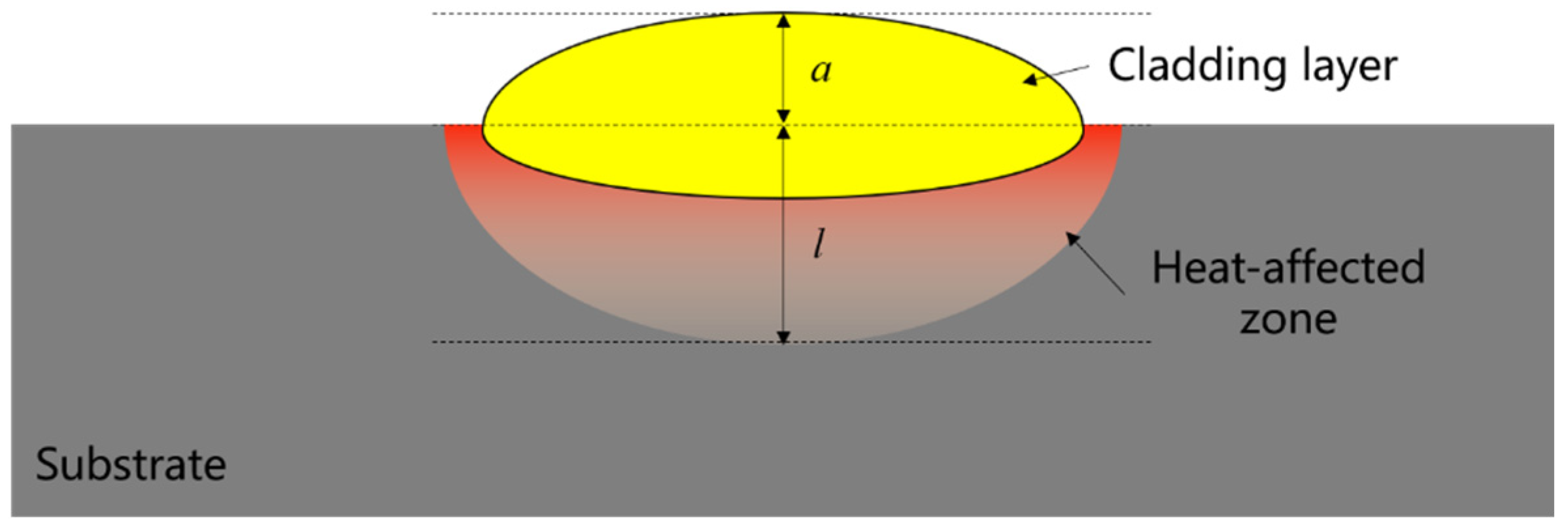
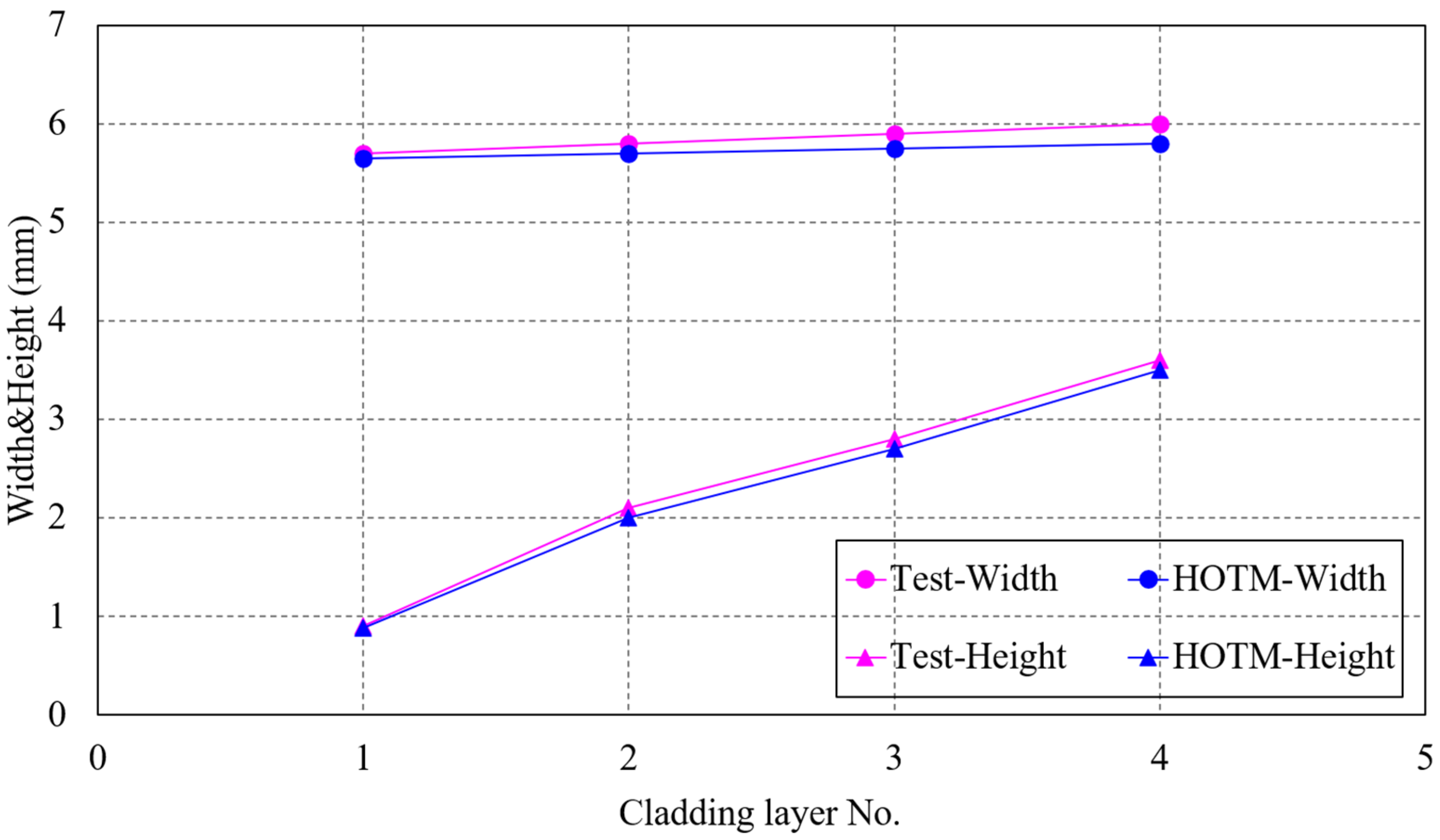
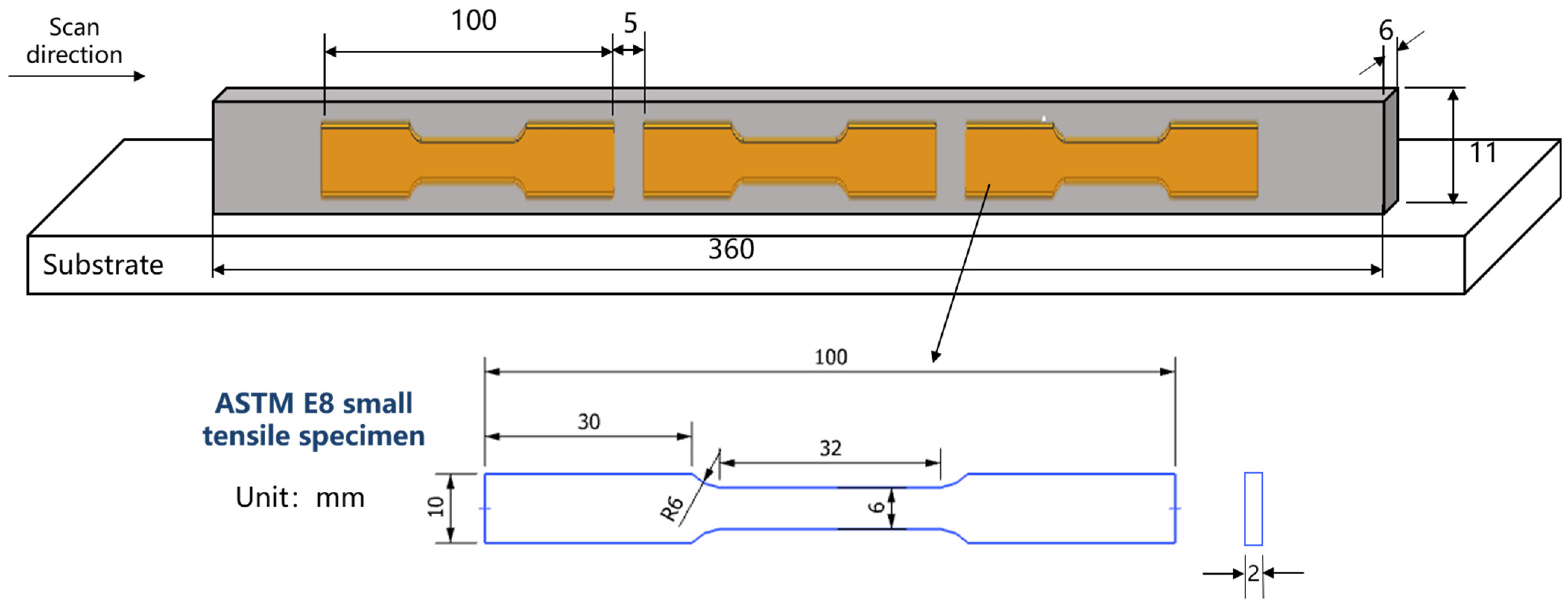
However, a large number of physical phenomena need to be solved in the meso-scale powder evolution model resulting in a high computational complexity and a low solution efficiency. The powder evolution model is currently only used in meso-scale research, which brings great difficulties to predict the macro-scale mechanical properties of the final components. How to predict the macro-scale mechanical properties according to a meso-scale model is the currently biggest problem. In this paper, this question is answered by a cladding stacking model based on the structural evolution of the heat-affected zone, and a process–structure–property multi-scale simulation framework. Though a series of experimental verifications, the relative error of the final mechanical property prediction is within 5.18%. This research achieves the final goal of predicting the macro-scale mechanical properties of fabricated components according to the given process parameters. This research can provide guidance for the design of numerical simulations and experiments, and provide a basis for the subsequent quantitative analysis of the process–structure–property relationship and the optimization of process parameters.

The remainder of this study is organized as follows. In Section 2, a cladding stacking model is proposed based on the structural evolution of the heat-affected zone and the verification experiments are carried out. In Section 3, a process–structure–property multi-scale numerical simulation framework is proposed based on this model, and the corresponding methods and theory are presented. In Section 4, a specific case is simulated based on the proposed cladding stacking model and the process–structure–property framework; finally, some conclusions are summarized in Section 5.

2. A Cladding Stacking Model

2.1. Model Introduction

To answer the question of how to predict the macro-scale mechanical properties of the final components using the printed local material simulated at the meso-scale, it is necessary to accurately understand the forming process of a component fabricated by the LMD. In this paper, through the deconstructive analysis of this process, a cladding stacking model is proposed to describe the forming process of a component.

During the laser cladding process, a heat-affected zone will be formed around the molten pool (Figure 1), which will affect the printed cladding layer to a certain extent. The scope of the heat-affected zone can be determined by the microstructure transition temperature of the cladding material. To facilitate the expression of whether the subsequent cladding layer has an impact on the existing cladding layer, a heat-affected zone coefficient R is defined as:

$$R=\frac{l}{a},$$

(1)

where l is the maximum depth of the heat-affected zone of a single layer, a is the thickness between the top surfaces of the single cladding layer and the substrate (Figure 1).

The heat-affected zone coefficient is affected by factors such as the type of the AM process, the laser power, and the laser diameter, etc. Another thing to note is the substrate temperature at the beginning of each printing is affected by the deposited idle time between consecutive layers, laser power, metal thermal conductivity, etc. Now assume that the R of a group of LMD process parameters is 2 and under these given process parameters, after the first cladding, the substrate temperature is the same value at the beginning of each subsequent printing.

When printing the first layer (Figure 2a), the first cladding layer forms the structure S1 at the initial temperature T1 of the substrate.

When printing the second layer (Figure 2b), S1 is the new substrate. Due to the irradiation of a laser, the new substrate temperature T2 > T1, resulting in a different structure S2 formed in the second layer; meanwhile, due to the influence of the heat-affected zone of S2, S1 will become S1′. Note that the different colors of the cladding layer in Figure 2 represent different structures.

When printing the third layer (Figure 2c), S2 is the new substrate. Currently, since the new substrate temperature T3 = T2, the structure S3 of the third layer will be the same as S2. The S1′ and S2 will become S1″ and S2′ under the influence of S3.

When printing the fourth layer (Figure 2d), the heat-affected zone of S4 just no longer affects the first layer structure S1″. The structure of the second, third and fourth layers will become S2″, S3’ = S2’, S4 = S2, respectively. It can be found that these three layers are the history of the structural evolution of S2, forming a basic cycle of S2, S2′, and S2″. The subsequent printing process can be treated as a recurring process according to this basic cycle until the end of the print (Figure 2e). Three typical structural regions will be formed inside the final fabricated component, namely the bottom region, the middle region, and the top region.

Therefore, if the history of the structural evolution in the heat-affected zone is known, the structure of the final fabricated component can be quickly predicted. For instance, for a prepared part shown in Figure 3, the overall structure on the right can be predicted rapidly under the abovementioned process parameters, even an irregular geometric component. The range of the heat-affected zone can be determined by the heat-affected zone coefficient R. Through the above analysis, it can be observed that if the R of a group of certain process parameters is N, the subsequent cladding layer will have an influence on the N-layer structures beneath it. To verify the correctness of this stacking model, a specific verification experiment is designed.

2.2. Experimental Verification

To verify the rationality of the stacking model, a LMD experiment that can reflect the structural evolution of the heat-affected zone is designed. A series of single-track multilayer printings were carried out under the same process parameters, and the metallographic morphology of each printed specimen was observed. The process parameters used in this study are shown in

Table 1. The main process parameters of the designed LMD experiment.

Laser Power (W)	Scan Speed (mm/min)	Powder Feed Rate (g/min)	Hatch Spacing (mm)	Powder Diameter (μm)
3000	600	10	0.5	53–180

. A total of eight specimens were printed, and the number of layers of each specimen is increased sequentially. Each layer was printed in a length of 20 mm (Figure 4). The width, height and grain structure of each specimen were measured and observed when it was cooled to room temperature after printing. The printing equipment used a 6000 W fiber laser with 4 nozzles. Since the Ti–6Al–4V alloy is a widely used material in the aerospace field, the study of the mechanical properties of Ti–6Al–4V prepared using traditional manufacturing processes is relatively mature. However, the mechanical properties of Ti–6Al–4V prepared using the LMD process are still in the research stage. To this end, this study takes the Ti–6Al–4V alloy as the object. The printed specimens are shown in Figure 5, and the cross-sectional metallographic observations are shown in Figure 6.

It can be observed that (Figure 6) the structure gradually grows upward from the substrate, showing a columnar crystal morphology on the whole with no obvious faults at each layer junction. Taking the final specimen 8 as an example, due to the contact with the substrate at the bottom of the structure, the cooling rate has a relatively large value, resulting in fine columnar grains formed in the bottom region. Due to the relatively small cooling rate in the middle region, the grains have sufficient time to grow. The middle region presents coarse columnar grains. The top region shows fine equiaxed crystal structures due to the cooling rate greater than the middle region and no subsequent printing. These phenomena are consistent with the prediction results of the cladding stacking model proposed in Section 2.1. Three different structural regions are formed at the top, middle and bottom. Especially from the fourth specimen, the differences of the three regions are obvious.

Through the measurement of the microstructure of the first layer (Figure 7), it is found that the coefficient of the heat-affected zone under this process parameter is about 2. According to the analysis of the cladding stacking model in Section 2.1, if the heat-affected zone coefficient is 2, the structure of layer 1 no longer changes when layer 4 is printed. Comparing the Figure 6d and subsequent microstructures, it can be found that the subsequent microstructures are basically consistent with the microstructures in Figure 6d, and the difference is mainly in the height of grains. For quantitative analysis, the average length and average width of grains of each specimen section were counted. The results (Figure 8) show that with the increase of the number of printed layers, the average length of the grain basically shows a linear growth trend, and it reaches 3.53 mm after the last printing. The average width grows rapidly during the first four printings, after which the size is basically stable, at 0.8–0.9 mm. These phenomena are consistent with the predictions obtained based on the cladding stacking model, which verifies its rationality.

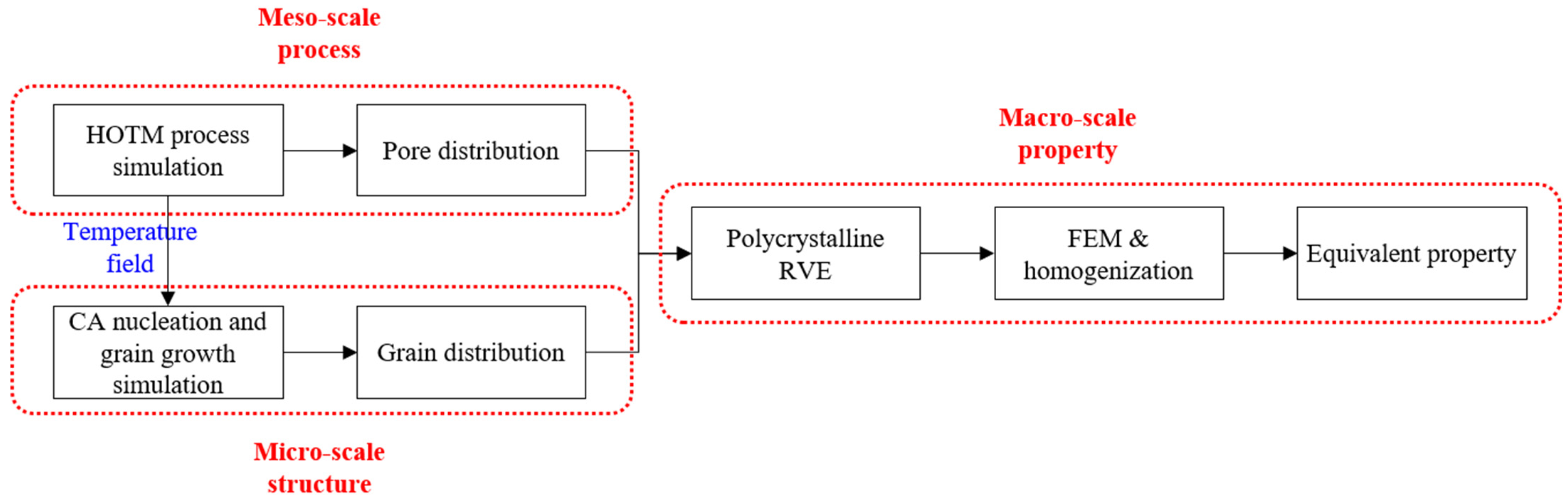
3. A Process–Structure–Property Multi-Scale Simulation Framework

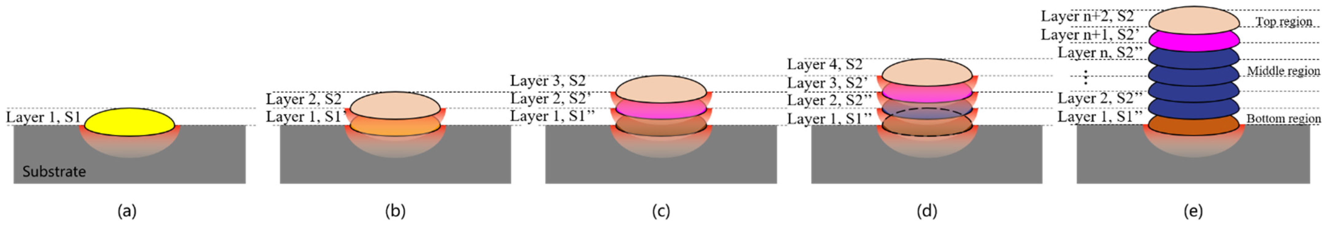
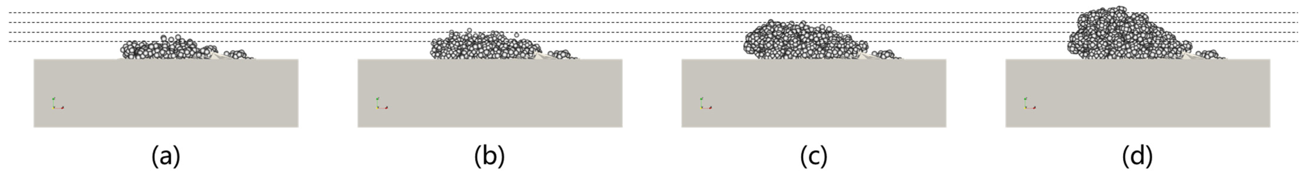
The cladding stacking model provides a basis for predicting the macro-scale mechanical properties of the final fabricated component by using meso-scale scale numerical simulation results. For example, under the process parameters of the Section 2.2, the meso-scale numerical simulation only needs to simulate the cladding processes of four layers. Then, the macroscopic mechanical properties of the final fabricated component can be obtained by combining the microstructure simulation and the equivalent method of macroscopic properties. Based on this, according to the actual printing process of LMD, this study establishes a multi-scale simulation framework that comprehensively considers the process–structure–property of additive manufacturing materials, as shown in Figure 9, by using the direct numerical simulation of meso-scale process as a bridge to link the simulation of the micro-scale structure and the calculation of macro-scale mechanical properties.

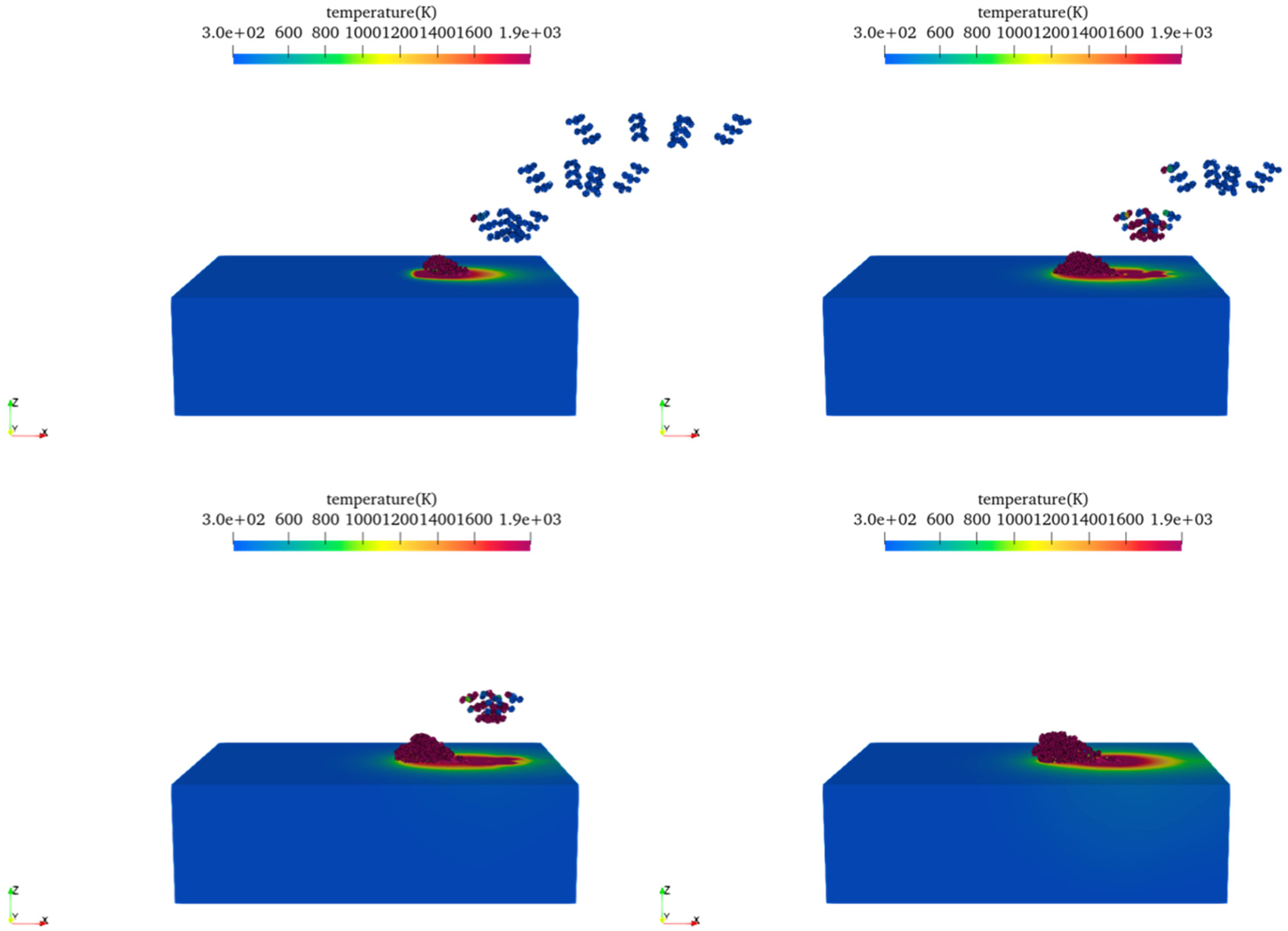
In the module of the meso-scale process simulation, HOTM is used to simulate the multi-layer printing process. The fields of temperature, fluid flow and stress, pores, deformations, and other information can be obtained, and the dynamic process of powders melting and solidification can be explored.

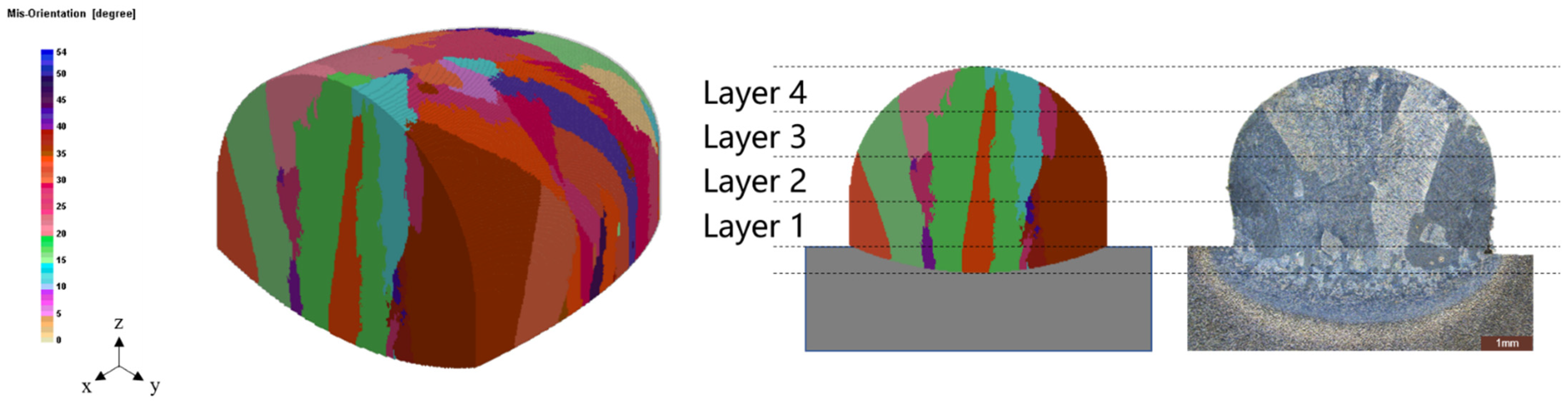
In module of the micro-scale structure simulation, the temperature field history obtained by the meso-scale process simulation can be used to simulate the microstructure formation. The main simulation methods are the Monte Carlo Method (MC) [23], the Cellular Automata Method (CA) [24,25,26] and the Phase Field Method (PF) [27,28,29,30]. Among them, CA is widely used in the numerical simulation of microstructure for its clear physical meaning, simple model, and high computational efficiency. In this study, CA is used to simulate the grain nucleation and growth process in the heat-affected zone and obtain the microstructural information such as grain size and orientation.

In the module of the macro-scale mechanical properties calculation, the macro-scale mechanical properties can be calculated by a Representative Volume Element (RVE) [31,32,33] containing the meso/micro-scale structural information and the homogenization theory [34,35].

Each module can set the verification tests. Numerical simulation methods for each module are described in detail below.

3.1. Simulation Method of Meso-Scale Powder Evolution Processes

The HOTM method is a Lagrangian meshfree method, which is characterized using the optimal transportation theory to discretize the time, using nodes with position information and material points with material information to disperse the space, and the shape function adopts a local maximum entropy interpolation function. HOTM does not have the problems of mesh distortion and reconstruction and by considering a phase-aware constitutive model the melting and solidification of the powder can be directly simulated under a unified Lagrangian coordinate system, which is a Direct Numerical Simulation (DNS) method. A detailed discussion of the HOTM theory can be found in [20,21,22]. Based on the HOTM theory, an additive manufacturing simulation platform ESCAAS is developed to simulate the meso-scale LMD multilayer cladding process.

3.1.1. Geometry Modeling

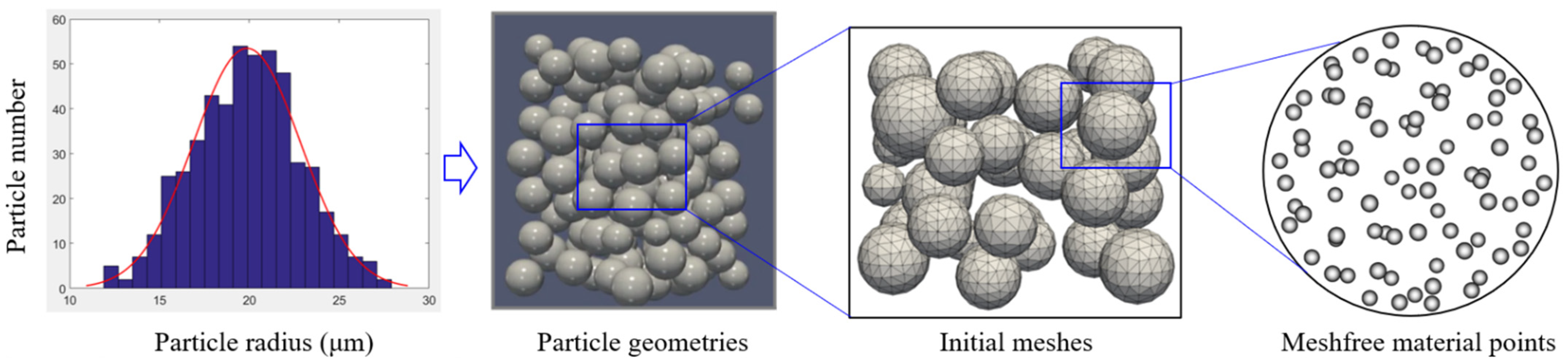
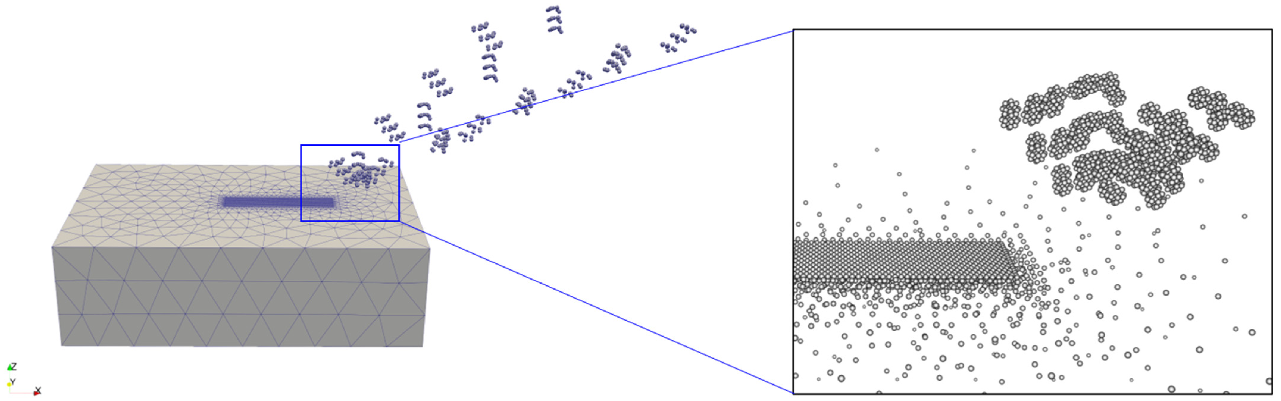
The Geometry Modeling module can automatically generate powder clusters by entering parameters such as the statistical distribution of powder particle size (for example, the mean and variance of the normal distribution), the powder cluster information (number, length, width, height), the minimum distance between the particles, etc., as shown in Figure 10. After the powder particle geometries are established, they are spatially discrete by the material points and the nodes. All calculations are performed on these material points and nodes.

3.1.2. Heat Source Model

The heat source is the input of energy to the model system and directly affects the accuracy of the simulation results. In the actual cladding process, the heat distribution on the spot of a laser is uneven and the heat source density is approximately normally distributed. Song et al. [36] and Kubiak et al. [37] found that the heat flux with ultra-Gaussian distributions can represent a more realistic laser beam. To this end, a heat source model including an ultra-Gaussian model was developed in ESCAAS:

$$q=\frac{AP}{\pi r^2}\exp \left(-2{\left(\frac{\sqrt{{(x-x_c)}^2+{(y-y_c)}^2}}{r}\right)}^n\right),$$

(2)

where q is the heat flux, A represents the surface absorption rate, P and r represent the laser power and laser radius, x_c and y_c are the laser center point locations, and the heat flux distribution shape can be selected by changing the order n.

3.1.3. Heat Transfer Model

The actual printing process includes three kinds of heat transfer phenomena: heat conduction, convection, and radiation. In ESCAAS, the classic Fourier thermal conduction model is adopted:

$$q=-\lambda \frac{\partial T}{\partial r}=-\lambda \left(\frac{\partial T}{\partial x}i+\frac{\partial T}{\partial y}j+\frac{\partial T}{\partial z}k\right),$$

(3)

where q is the heat flux in the r direction, which is perpendicular to the isothermal plane, and the negative sign indicates that the heat transfer direction is opposite to the temperature gradient direction, $\lambda$ is the thermal conductivity and T is the temperature.

The thermal convection model adopts Newton’s law of cooling. To consider the energy loss caused by evaporation, the latent heat of evaporation is regarded as the convective heat flux of the powder/substrate and the environment. Thus, a combined convective heat flux can be described as:

$$q=h\left(T-T_0\right),$$

(4)

where h is the combined convection heat transfer coefficient and T₀ is the ambient temperature.

The Stefan Boltzmann’s law is used to apply the radiant heat flow at surface nodes:

$$q=\kappa \epsilon \left(T^4-T_0^4\right),$$

(5)

where the Stefan Boltzmann constant $\kappa =5.67\times {10}^{-8} \mathrm{W}/({\mathrm{m}}^2·{\mathrm{K}}^4)$, $\epsilon$ is the emissivity of the object.

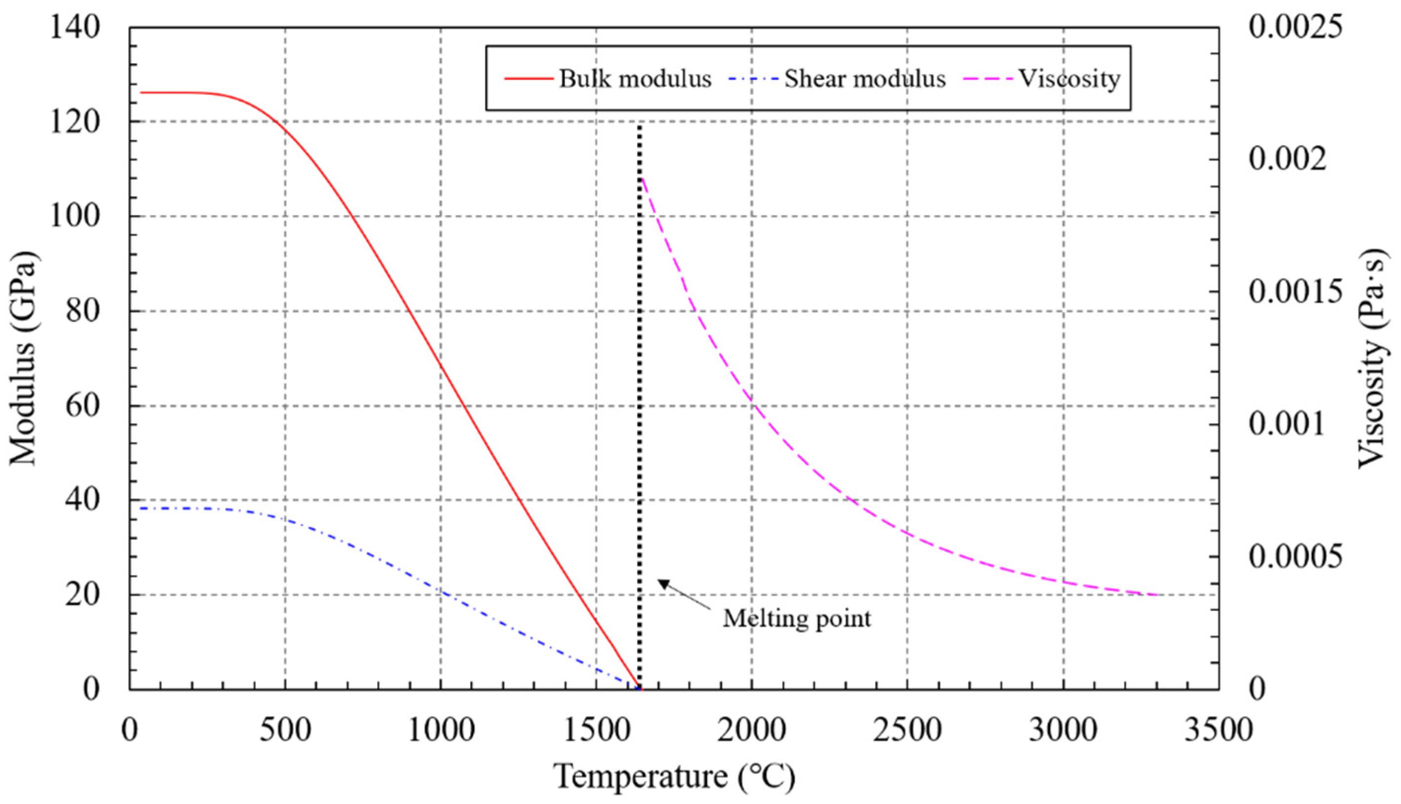
3.1.4. Phase Transition Model

During the phase transition, there is a phase transition region $T_m\mp \mathsf{\Delta }T$, and when the temperature reaches this region, the phase transition begins. A phase transition function is used to describe the smooth transition between two phases:

$$\alpha (T)=\frac{1}{2}\left[1+\mathrm{erf}\left(\frac{T-T_m}{\sqrt{2}\sigma }\right)\right],$$

(6)

where T_m is the melting temperature, σ is the transition interval standard deviation. For example, for pure solids α (T) = 0, and for pure liquids α(T) = 1.

The phase transition function can be used to relate the thermal material parameters to the phase state. In ESCAAS, the specific heat capacity $C(T)$, the thermal conductivity $\lambda (T)$ and the coefficient of thermal expansion $\theta \left(T\right)$ are defined as functions of the temperature and phase state:

$$C(T)=C_{\mathrm{phase}1}\left(1-\alpha (T)\right)+C_{\mathrm{phase}2}\alpha (T)+{\rho }_{0}L\frac{d\alpha (T)}{dT},$$

(7)

$$\lambda (T)={\lambda }_{\mathrm{phase}1}\left(1-\alpha (T)\right)+{\lambda }_{\mathrm{phase}2}\alpha (T),$$

(8)

$$\theta (T)={\theta }_{\mathrm{phase}1}\left(1-\alpha (T)\right)+{\theta }_{\mathrm{phase}2}\alpha (T),$$

(9)

where ${\rho }_0$ is the density of a material, and L is the latent heat during the phase transition.

3.1.5. Material Model

The LMD process involves the phase transformation, so a phase-sensitive constitutive model should be defined. In ESCAAS, the constitutive models of solid and liquid phases are defined separately.

When the material is in the solid phase, its constitutive model is:

$${\sigma }_{ij}=\frac{K\left(T\right)}{2}\left(J-\left(1+3\theta \left(T\right)\cdot \mathrm{\Delta }T\right)\frac{1}{J}\right){\delta }_{ij}+2\mu \left(T\right){\epsilon }_{ij}^{dev},$$

(10)

where ${\sigma }_{ij}$ is stress, $K\left(T\right)$ is the volumetric modulus, $\mu \left(T\right)$ is the shear modulus, ${\delta }_{ij}$ is the Kronecker delta, J is the Jacobian of the local material, ${\epsilon }_{ij}^{dev}$ is the deviatoric strain.

When the material is in the liquid phase, its constitutive model is the viscoelastic model with Murnaghan–Tait equation of state:

$${\sigma }_{ij}=\left(-\frac{\chi \left(T\right)}{\gamma \left(T\right)}\left(J^{-\gamma \left(T\right)}-1\right)-P_0\right){\delta }_{ij}+2\eta \left(T\right){\dot{\epsilon }}_{ij},$$

(11)

$$\chi \left(T\right)=b{T}^{\alpha 1},$$

(12)

$$\gamma \left(T\right)=c{T}^{\alpha 2},$$

(13)

where $\chi \left(T\right)$ and $\gamma \left(T\right)$ are temperature-dependent functions that represent the compressibility of a material, $b{,}_{}c{,}_{}\alpha 1{,}_{}\alpha 2$ are the corresponding coefficients, $\eta \left(T\right)$ is the viscosity, $P_0$ is the ambient pressure, and ${\dot{\epsilon }}_{ij}$ is the strain rate.

3.2. Simulation Method of Microstructure Formations

The microstructure has a great impact on the mechanical properties of a material. According to the temperature field in the meso-scale process simulation, the simulation of the micro-scale structure can be performed. In this study, CA is used to simulate the microstructure formation process. According to the theory of solidification, the formation of micro-scale structures includes two processes: grain nucleation and growth. To simulate these two processes, the corresponding quantitative models are required.

3.2.1. Nucleation Model

The nucleation is critical for the simulation of microstructures and directly affects the number of grains at the end of the solidification. According to the theory of the nucleation, in the process of liquid–solid phase transition of metals, there are two kinds of nucleation mechanisms, the homogeneous nucleation and the heterogeneous nucleation. The solidification of a metal is usually in the latter way in practice. Throughout the actual solidification process, the nuclei are formed continuously until the liquid metal disappears completely. This study uses the Rappaz continuous heterogeneous nucleation model [38] to simulate the nucleation process. The model holds that at a certain degree of supercooling $\mathrm{\Delta }T$, the nucleation phenomenon occurs in a series of different nucleation sites and the change of the nucleation density $dn/d(\mathrm{\Delta }T)$ satisfies the Gaussian probability distribution. The nucleation density can be obtained by the integral formula (14) at a certain degree of supercooling $\mathrm{\Delta }T$:

$$n(\mathrm{\Delta }T)={\displaystyle {\int }_0^{\mathrm{\Delta }T}\frac{dn}{d(\mathrm{\Delta }T)}}d(\mathrm{\Delta }T),$$

(14)

$$\frac{dn}{d(\mathrm{\Delta }T)}=\frac{n_{\max }}{\sqrt{2\pi }·\mathrm{\Delta }{T}_{\sigma }}\exp \left(-\frac{1}{2}{\left(\frac{\mathrm{\Delta }T-\mathrm{\Delta }{T}_n}{\mathrm{\Delta }{T}_{\sigma }}\right)}^2\right),$$

(15)

where $\mathrm{\Delta }{T}_n$ is the average of supercooling, $\mathrm{\Delta }{T}_{\sigma }$ is the standard deviation of supercooling, and $n_{\max }$ is the maximum nucleation density.

3.2.2. Growth Model

Once the nucleus is formed, it begins to grow until all the nuclei meet each other. The process of continuous growth of the nucleus is the process of gradual expansion of the solid-state interface. This study uses a simplified KGT model [39] to simulate the nucleus growth process:

$$v=\alpha \mathrm{\Delta }{T}^2+\beta \mathrm{\Delta }{T}^3,$$

(16)

where $v$ is the growth velocity of the crystal interface, $\alpha {,}_{}\beta$ are the constants determined by the thermal physical properties of a metal.

3.3. Prediction Method of Mechanical Properties of Macro-Scale Components

The material fabricated by LMD often contains defects such as inclusions, pores and for multiphase materials they also contain different crystal phases. Therefore, the materials fabricated by LMD are heterogeneous on the microscopic scale. The homogenization of heterogeneous materials to gain the macro-scale mechanical properties has been studied for decades [31,32,33,34,35], in which the calculation of the equivalent stiffness of a material has been relatively mature, and the calculation of the equivalent strength is still in the research stage. This study takes the macro-scale Young’s modulus of the material as an example to illustrate the method used in this study. Other mechanical properties can also be included in this multiscale simulation framework.

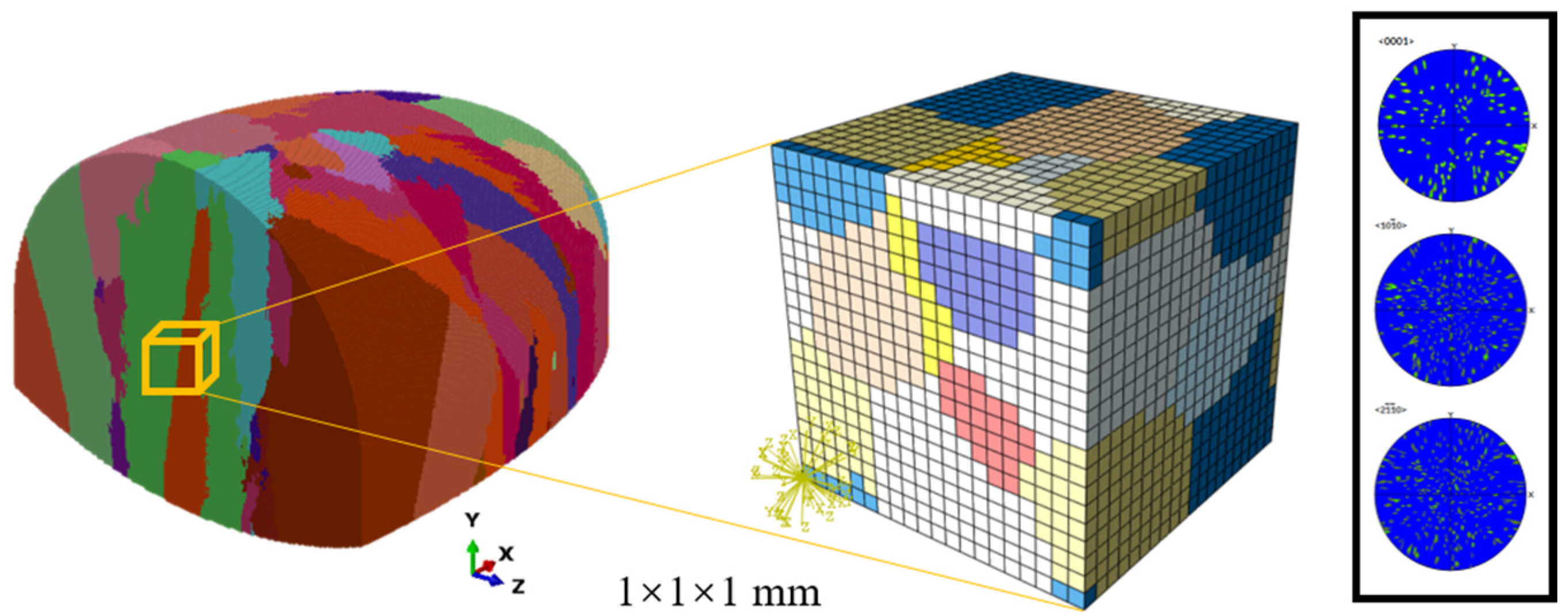
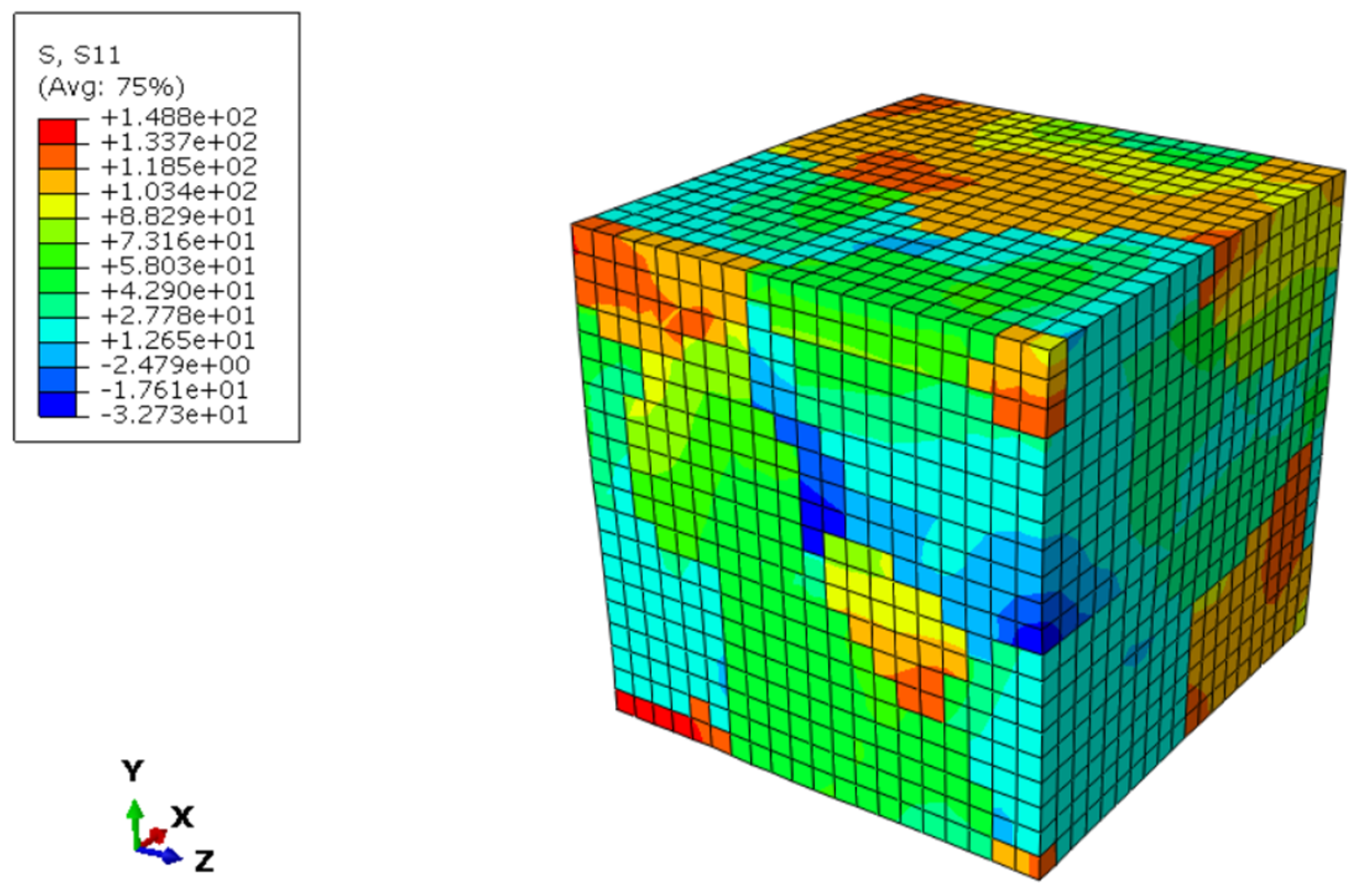
The macro-scale Young’s modulus of a material is determined by the internal structure. An RVE can be established to link the micro and the macro, which contains detailed meso/micro-structure information, such as the distribution of the grains, pores, and the material properties of different phases. The stress of each node in the RVE can be obtained by applying a uniform strain $\overline{\epsilon }$ on the RVE boundary and the corresponding finite element mechanical solution. Based on the homogenization technology, an average stress $\overline{\sigma }$ can be calculated, and the macro-scale equivalent Young’s modulus $\overline{C}$ can be obtained according to the equation:

$$\overline{\sigma }=\overline{C}\cdot \overline{\epsilon }.$$

(17)

4. Simulation Cases, Results and Discussion

4.1. Simulation of Meso-Scale Processes

The simulation in this section is based on the experiments of Section 2.2. It has been concluded that only four layers need to be simulated in the meso-scale simulation. Therefore, according to the powder size and process parameters in the experiments of Section 2.2, a meso-scale model for HOTM to simulate the LMD multilayer printing process is established, including four-layer powder clusters and a substrate, as shown in Figure 11. In the HOTM simulation, three velocity components in the Cartesian coordinates are applied to each cluster of powder to simulate the powder flow aggregation behavior. The material parameters of Ti–6Al–4V for the HOTM calculation are listed in

Table 2. Material parameters of Ti–6Al–4V for the HOTM simulation.

Parameter	Value	Parameter	Value
Specific heat capacity of solid (J/(kg·K))	611	Latent heat melting (kJ/kg)	286
Specific heat capacity of liquid (J/(kg·K))	900	Latent heat vaporization (kJ/kg)	9700
Thermal conductivity of solid (W/(m·K))	6.8	Coefficient of compressibility, b	2 × 1010
Thermal conductivity of liquid (W/(m·K))	32.5	Coefficient of compressibility, c	47.65
Coefficient of thermal expansion of solid (/℃)	9.1 × 10−6	Coefficient of compressibility, α1	−1
Coefficient of thermal expansion of liquid (/℃)	1.6 × 10−5	Coefficient of compressibility, α2	−0.354
Melting temperature (℃)	1650	Bulk modulus (GPa)	See Figure 12
Boiling temperature (℃)	3260	Shear modulus (GPa)	See Figure 12
Convective heat conduction coefficient (W/(m2·K))	50	Viscosity (Pa·s)	See Figure 12

.

From the simulation results, it can be observed (Figure 13) that the powder clusters gradually converge in the air into the laser irradiation range, heated and molten. The surface of the substrate forms a molten pool, and the molten powders are fused with it to form a cladding layer. The height of the fabricated material increases layer by layer. The morphologies of each layer after cladding are shown in Figure 14.

To quantitatively verify the accuracy of the simulations, the maximum height and maximum width of the experimental and simulated cladding layers were measured separately, as shown in Figure 15. It can be observed that with the increase of the number of printing layers, the height of the fabricated material basically shows an obviously linear increasing trend, while the width varies less. The simulation results of the HOTM process are in good agreement with the experimental data. The maximum relative errors of the width and the height are within 3.33% and 4.76%, respectively.

4.2. Simulation of Microstructures

According to the simulation results of the meso-scale process, a multilayer microstructure simulation model can be established. The formation of the four-layer structures is simulated based on the temperature field of the meso-scale simulation, as shown in Figure 16. The Ti–6Al–4V thermal material parameters used for the CA simulation are listed in

Table 3. The nucleation and grain growth simulation parameters.

Parameter	Value
Liquidus temperature (℃)	1650
Solidus temperature (℃)	1554
Maximum nucleation density, $n_{\max }$ (m−3)	1 × 109
Average of supercooling, $\mathrm{\Delta }{T}_n$ (k)	32
Standard deviation of supercooling, $\mathrm{\Delta }{T}_{\sigma }$ (k)	8
Coefficient of growth, α	0
Coefficient of growth, β	3.19 × 10−5
Cell size (μm)	20

.

By comparing the average grain length and width of the cross-section (

Table 4. The experiment and simulation comparison of the four-layer microstructures.

	Experiment	CA	Relative Error (%)
Average length (mm)	1.97	2.01	2.03
Average width (mm)	0.85	0.81	4.71

), it is found that the maximum relative errors are within 2.03% and 4.71%, respectively, and the simulation results are in good agreement with the experimental metallographic observations, which verifies the accuracy of the micro-scale structure simulation.

4.3. Prediction of Macro-Scale Mechanical Properties

Based on the process parameters in Section 2.2, a 360 × 6 × 11 mm brick component was fabricated (Figure 17) and cooled to the room temperature. To consider the difference in the mechanical properties of the component in the length direction, three small-size standard tensile test specimens (Figure 17) were cut and sampled in the length direction for the static unidirectional tensile test to obtain the macro-scale tensile Young’s modulus according to the international standard ASTM E8. The average of the Young’s modulus of the three specimens is taken as the macro-scale Young’s modulus of the brick component.

Based on the analysis in Section 2, there are three typical microstructure regions in the fabricated component. Since the bottom and top materials are removed when sampling the standard specimens, the structure of the standard specimens belongs to the middle-region structure. By extracting the middle structure in the micro-scale structure simulation, a polycrystalline RVE analysis model was established (Figure 18).

The establishment of the polycrystalline RVE requires the nucleus position and grain orientation information, which can be extracted from the CA simulation. The extracted data are then passed to an open-source software Dream3D to build the polycrystalline RVE analysis model for finite element mechanical calculations. The ABAQUS software was used for the mechanical calculation in this study. Note that Ti–6Al–4V is a two-phase alloy. The microstructure of Ti–6Al–4V produced by LMD is dominated by hexagonal close-packed (hcp) α grains. The β phase mainly exists in the high temperature environment. To simplify the RVE model and computational complexity, the β phase was ignored in this study. The material properties used in the Finite Element Analysis (FEA) (

Table 5. α transverse isotropic elastic tensor parameter of the phase [40].

Cij	Value (GPa)
C11 = C22	170
C33	204
C12 = C21	98
C13 = C31 = C23 = C32	86
C44	72
C55 = C66	102
Other Cij	0

) are the transverse isotropic material properties of the α phase from the literature [40]. By applying an x-direction uniform strain boundary, a static tensile FEA was performed on the polycrystalline RVE model. Figure 19 shows the x-direction stress distribution. Through the homogenization theory, the calculated equivalent macro-scale Young’s modulus is 65.72 GPa (

Table 6. The test and simulation value of Young’s modulus of standard x-direction static tension.

Tensile Specimen No.	Experiment (GPa)	Experimental Average (GPa)	Simulation (GPa)	Relative Error (%)
1	69.22	69.31	65.72
2	69.45			5.18
3	69.25

). The relative error between the simulation results and the test results is 5.18%, which shows the effectiveness of the cladding stacking model and the multiscale simulation framework.

5. Conclusions

This study finds an approach to predict the macro-scale mechanical properties of the fabricated component according to the process parameters by a cladding layer stacking model including the microstructural evolution history of the heat-affected zone and a process–structure–property multi-scale simulation framework. The following conclusions are listed through the research.

• The range of the heat-affected zone in LMD can be determined by a heat-affected zone coefficient R. If the R is N, the subsequent cladding layer will have an influence on the N-layer structures beneath it;
• Based on the structural evolution history in the heat-affected zone, the cladding stacking model can quickly predict the overall structure of the fabricated component;
• The process–structure–property multi-scale simulation framework based on the cladding stacking model can predict the macro-scale mechanical properties of the final fabricated component according to the process parameters;
• Under multi-layer printings, the structure in the cladding layers gradually grows continuously from the substrate, showing a columnar crystal morphology on the whole, and finally forming three typical microstructure regions of the top, middle and bottom due to the influence of the heat-affected zone and heat dissipation conditions;
• The height of the fabricated material shows a linear increasing trend with the number of layers; the width is less affected by the number of layers; and
• The length of the cross-section grain of the fabricated material shows a linear growth trend with the number of layers; the width increases rapidly within the heat-affected zone and then reaches stability.

References

1. Arcella, F.G.; Froes, F.H. Producing titanium aerospace components from powder using laser forming. JOM-J. Miner. Met. Mater. Soc. 2000, 52, 28–30. [Google Scholar] [CrossRef]
2. Gu, D.D.; Meiners, W.; Wissenbach, K.; Poprawe, R. Laser additive manufacturing of metallic components: Materials, processes and mechanisms. Int. Mater. Rev. 2012, 57, 133–164. [Google Scholar] [CrossRef]
3. Wang, H. Materials’ fundamental issues of laser additive manufacturing for high-performance large metallic components. Hangkong Xuebao/Acta Aeronaut. Astronaut. Sin. 2014, 35, 2690–2698. [Google Scholar]
4. Dutta, B.; Froes, F.H. The Additive Manufacturing (AM) of titanium alloys. Met. Powder Rep. 2017, 72, 96–106. [Google Scholar] [CrossRef]
5. Oztan, C.; Coverstone, V. Utilization of additive manufacturing in hybrid rocket technology: A review. Acta Astronaut. 2021, 180, 130–140. [Google Scholar] [CrossRef]
6. Brennan, M.C.; Keist, J.S.; Palmer, T.A. Defects in Metal Additive Manufacturing Processes. J. Mater. Eng. Perform. 2021, 30, 4808–4818. [Google Scholar] [CrossRef]
7. Rashkovets, M.; Mazzarisi, M.; Nikulina, A.A.; Casalino, G. Analysis of laser direct stainless steel powder deposition on Ti6Al4V substrate. Mater. Lett. 2020, 274, 128064. [Google Scholar] [CrossRef]
8. Hu, Y.N.; Wu, S.C.; Withers, P.J.; Zhang, J.; Bao, H.Y.X.; Fu, Y.N.; Kang, G.Z. The effect of manufacturing defects on the fatigue life of selective laser melted Ti-6Al-4V structures. Mater. Des. 2020, 192, 108708. [Google Scholar] [CrossRef]
9. Yan, W.T.; Lin, S.; Kafka, O.L.; Lian, Y.P.; Yu, C.; Liu, Z.L.; Yan, J.H.; Wolff, S.; Wu, H.; Ndip-Agbor, E.; et al. Data-driven multi-scale multi-physics models to derive process-structure-property relationships for additive manufacturing. Comput. Mech. 2018, 61, 521–541. [Google Scholar] [CrossRef]
10. Yang, Y.P.; Babu, S.S. An Integrated Model to Simulate Laser Cladding Manufacturing Process for Engine Repair Applications. Weld World 2010, 54, R298–R307. [Google Scholar] [CrossRef]
11. Costa, L.; Vilar, R.; Reti, T.; Deus, A.M. Rapid tooling by laser powder deposition: Process simulation using finite element analysis. Acta Mater. 2005, 53, 3987–3999. [Google Scholar] [CrossRef]
12. Yuan, P.P.; Gu, D.D.; Dai, D.H. Particulate migration behavior and its mechanism during selective laser melting of TiC reinforced Al matrix nanocomposites. Mater. Des. 2015, 82, 46–55. [Google Scholar] [CrossRef]
13. Manvatkar, V.; De, A.; DebRoy, T. Spatial variation of melt pool geometry, peak temperature and solidification parameters during laser assisted additive manufacturing process. Mater. Sci. Tech. 2015, 31, 924–930. [Google Scholar] [CrossRef]
14. Raghavan, A.; Wei, H.L.; Palmer, T.A.; DebRoy, T. Heat transfer and fluid flow in additive manufacturing. J. Laser Appl. 2013, 25, 052006. [Google Scholar] [CrossRef] [Green Version]
15. Schoinochoritis, B.; Chantzis, D.; Salonitis, K. Simulation of metallic powder bed additive manufacturing processes with the finite element method: A critical review. Proc. Inst. Mech. Eng. Part B J. Eng. Manuf. 2017, 231, 96–117. [Google Scholar] [CrossRef]
16. Balu, P.; Leggett, P.; Kovacevic, R. Parametric study on a coaxial multi-material powder flow in laser-based powder deposition process. J. Mater. Process. Technol. 2012, 212, 1598–1610. [Google Scholar] [CrossRef]
17. Yan, W.T.; Qian, Y.; Ge, W.J.; Lin, S.; Liu, W.K.; Lin, F.; Wagner, G.J. Meso-scale modeling of multiple-layer fabrication process in Selective Electron Beam Melting: Inter-layer/track voids formation. Mater. Des. 2018, 141, 210–219. [Google Scholar] [CrossRef]
18. Khairallah, S.A.; Anderson, A.T.; Rubenchik, A.; King, W.E. Laser powder-bed fusion additive manufacturing: Physics of complex melt flow and formation mechanisms of pores, spatter, and denudation zones. Acta Mater. 2016, 108, 36–45. [Google Scholar] [CrossRef] [Green Version]
19. Wessels, H.; Weissenfels, C.; Wriggers, P. Metal particle fusion analysis for additive manufacturing using the stabilized optimal transportation meshfree method. Comput. Methods Appl. Mech. Eng. 2018, 339, 91–114. [Google Scholar] [CrossRef]
20. Wang, H.; Liao, H.M.; Fan, Z.Y.; Fan, J.; Stainier, L.; Li, X.B.; Li, B. The Hot Optimal Transportation Meshfree (HOTM) method for materials under extreme dynamic thermomechanical conditions. Comput. Methods Appl. Mech. Eng. 2020, 364, 112958. [Google Scholar] [CrossRef]
21. Fan, Z.Y.; Li, B. Meshfree Simulations for Additive Manufacturing Process of Metals. Integr. Mater. Manuf. Innov. 2019, 8, 144–153. [Google Scholar] [CrossRef]
22. Fan, Z.Y.; Wang, H.; Huang, Z.D.; Liao, H.M.; Fan, J.; Lu, J.; Liu, C.; Li, B. A Lagrangian meshfree mesoscale simulation of powder bed fusion additive manufacturing of metals. Int. J. Numer. Methods Eng. 2021, 122, 483–514. [Google Scholar] [CrossRef]
23. Rodgers, T.M.; Madison, J.D.; Tikare, V. Simulation of metal additive manufacturing microstructures using kinetic Monte Carlo. Comput. Mater. Sci. 2017, 135, 78–89. [Google Scholar] [CrossRef]
24. Gandin, C.A.; Rappaz, M.; Tintillier, R. 3-Dimensional simulation of the grain formation in investment castings. Met. Mater. Trans. A 1994, 25, 629–635. [Google Scholar] [CrossRef] [Green Version]
25. Gandin, C.A.; Rappaz, M. A 3D cellular automaton algorithm for the prediction of dendritic grain growth. Acta Mater. 1997, 45, 2187–2195. [Google Scholar] [CrossRef]
26. Yin, H.; Felicelli, S.D. Dendrite growth simulation during solidification in the LENS process. Acta Mater. 2010, 58, 1455–1465. [Google Scholar] [CrossRef]
27. Steinbach, I.; Pezzolla, F.; Nestler, B.; Seeßelberg, M.; Prieler, R.; Schmitz, G.J.; Rezende, J.L.L. A phase field concept for multiphase systems. Phys. D Nonlinear Phenom. 1996, 94, 135–147. [Google Scholar] [CrossRef]
28. Steinbach, I.; Beckermann, C.; Kauerauf, B.; Li, Q.; Guo, J. Three-dimensional modeling of equiaxed dendritic growth on a mesoscopic scale. Acta Mater. 1999, 47, 971–982. [Google Scholar] [CrossRef]
29. Fallah, V.; Amoorezaei, M.; Provatas, N.; Corbin, S.F.; Khajepour, A. Phase-field simulation of solidification morphology in laser powder deposition of Ti-Nb alloys. Acta Mater. 2012, 60, 1633–1646. [Google Scholar] [CrossRef]
30. Sahoo, S.; Chou, K. Phase-field simulation of microstructure evolution of Ti-6Al-4V in electron beam additive manufacturing process. Addit. Manuf. 2016, 9, 14–24. [Google Scholar] [CrossRef]
31. Drugan, W.J.; Willis, J.R. A micromechanics-based nonlocal constitutive equation and estimates of representative volume element size for elastic composites. J. Mech. Phys. Solids 1996, 44, 497–524. [Google Scholar] [CrossRef]
32. Ren, Z.Y.; Zheng, Q.S. A Quantitative study of minimum sizes of representative volume elements of cubic polycrystals—Numerical experiments. J. Mech. Phys. Solids 2002, 50, 881–893. [Google Scholar] [CrossRef]
33. Kanit, T.; Forest, S.; Galliet, I.; Mounoury, V.; Jeulin, D. Determination of the size of the representative volume element for random composites: Statistical and numerical approach. Int J. Solids Struct 2003, 40, 3647–3679. [Google Scholar] [CrossRef]
34. Willis, J.R. Variational and Related Methods for the Overall Properties of Composites. Adv. Appl. Mech. 1981, 21, 1–78. [Google Scholar]
35. Xing, Y.; Meng, L.; Huang, Z.; Gao, Y. A Novel Efficient Prediction Method for Microscopic Stresses of Periodic Beam-like Structures. Aerospace 2022, 9, 553. [Google Scholar] [CrossRef]
36. Song, X.L.; Li, B.B.; Guo, Z.; Wang, S.Y.; Cai, D.F.; Wen, J.G. Influences of pump beam distribution on thermal lensing spherical aberration in an LD end-pumped Nd:YAG laser. Opt. Commun. 2009, 282, 4779–4783. [Google Scholar] [CrossRef]
37. Kubiak, M.; Piekarska, W.; Stano, S. Modelling of laser beam heat source based on experimental research of Yb:YAG laser power distribution. Int. J. Heat Mass Transf. 2015, 83, 679–689. [Google Scholar] [CrossRef]
38. Rappaz, M.; Gandin, C.A. Probabilistic modelling of microstructure formation in solidification processes. Acta Metall. Mater. 1993, 41, 345–360. [Google Scholar] [CrossRef]
39. Kurz, W.; Giovanola, B.; Trivedi, R. Theory of microstructural development during rapid solidification. Acta Metall. 1986, 34, 823–830. [Google Scholar] [CrossRef]
40. Thomas, J.; Groeber, M.; Ghosh, S. Image-based crystal plasticity FE framework for microstructure dependent properties of Ti-6Al-4V alloys. Mater. Sci. Eng. A 2012, 553, 164–175. [Google Scholar] [CrossRef]
Figure 1. Schematic showing the cladding layer and the heat-affected zone.
Aerospace 09 00656 g001
Figure 2. Schematic showing the structural evolution process of the LMD multilayer printing: (ad) represent the solidified structure of the cladding layers by 1,2,3,4 printing, respectively; (e) represents the overall solidified structure of the cladding layers by n + 2 printing.
Aerospace 09 00656 g002
Figure 3. Prediction of the overall structure of fabricated components based on the structural evolution history of the heat-affected zone: (a) represents the prediction of a regular part; (b) represents the prediction of an irregular part.
Aerospace 09 00656 g003
Figure 4. Schematic of the designed LMD experiment.
Aerospace 09 00656 g004
Figure 5. The printed specimens and the cut section for metallographic observations.
Aerospace 09 00656 g005
Figure 6. Metallographic observations on the cross-section of each specimen: (ah) represent the solidified structure of each specimen.
Aerospace 09 00656 g006
Figure 7. The range of the heat-affected zone under the given process parameters.
Aerospace 09 00656 g007
Figure 8. The average length and average width of grains.
Aerospace 09 00656 g008
Figure 9. The process–structure–property multi-scale simulation framework.
Aerospace 09 00656 g009
Figure 10. The geometry modeling of powder particles with meshfree discrete.
Aerospace 09 00656 g010
Figure 11. The discrete model for the HOTM simulation.
Aerospace 09 00656 g011
Figure 12. The modulus and viscosity of Ti–6Al–4V.
Aerospace 09 00656 g012
Figure 13. The temperature field distribution in the four-layer cladding process.
Aerospace 09 00656 g013
Figure 14. The simulated cladding layers by HOTM: (ad) represent the solidified material by 1,2,3,4 printing, respectively.
Aerospace 09 00656 g014
Figure 15. The width and height of the cladding layer of the HOTM simulation and the experiment.
Aerospace 09 00656 g015
Figure 16. The 4-layer microstructure by the CA simulation.
Aerospace 09 00656 g016
Figure 17. Schematic showing the fabricated component and samplings.
Aerospace 09 00656 g017
Figure 18. The polycrystalline RVE mesh model for FEA.
Aerospace 09 00656 g018
Figure 19. The S11 stress distribution of the polycrystalline RVE under the x-direction tension.
Aerospace 09 00656 g019