Fractional-Order Sliding Mode Control Method for a Class of Integer-Order Nonlinear Systems

Abstract

In this study, the problem of the stabilisation of a class of nonautonomous nonlinear systems was studied. First, a fractional stability theorem based on a fractional-order Lyapunov inequality was formulated. Then, a novel fractional-order sliding surface, which was a generalisation of integral, first-order, and second-order sliding surfaces with varying fractional orders, was proposed. Finally, a fractional-order sliding mode-based control for a class of nonlinear systems was designed. The stability property of the system with the proposed method was easily proven as a fractional Lyapunov direct method by the fractional stability theorem. As an illustration, the method was used as a fractional guidance law with an impact angle constraint for a manoeuvring target. Simulation results demonstrated the applicability and efficiency of the proposed method.

1. Introduction

Fractional calculus is a generation of classical calculus that extends the order of derivatives and integrals to non-integers. Fractional calculus is an old topic but has gained increasing attention from researchers. In recent years, fractional calculus has found a wide range of applications in real-world systems such as viscoelastic models of materials [1], bioengineering [2], finance [3], and electronic circuits [4]. Fractional calculus is also widely used in control engineering [5,6,7]. The fractional-order proportional–integral–derivative (PID) controller, which has a much larger stability region than the classical PID type, has been extensively researched [6,8,9]. In addition, fractional-order finite-time control methods for nonlinear fractional-order systems have been discussed [10,11,12].

Recently, the combination of fractional calculus theory with sliding mode control methods, called fractional-order sliding mode control (FO-SMC), has received increasing interest from researchers [13,14,15,16,17,18,19]. Sliding mode control (SMC) is a well-known variable structure control method that has been widely used in the control of nonlinear systems [20,21,22,23]. SMC has many advantages, such as fast response, good transient performance, robustness to uncertainties, and insensitivity to bounded disturbances [24]. The SMC process can be divided into two phases: the sliding phase and reaching phase [24]. Once the sliding surface is reached, the robustness of the system is achieved. FO-SMC has been extensively applied in fractional-order systems and has recently found an increasing number of applications in integer-order systems. The pioneer work on FO-SMC was executed by Machado et al. [25], who studied fractional variable structure controllers and applied the method in a mechanical manipulator. Aghababa et al. [13] proposed a fractional integral-type sliding surface and applied a fractional SMC to stabilise uncertain fractional-order chaotic systems. Delavari et al. [14] designed a sliding proportional derivative surface and proposed a fuzzy fractional-order sliding mode controller for nonlinear systems. Sheng et al. [15] studied an FO-SMC-based guidance law with an impact angle constraint for lifting an unpowered re-entry vehicle to a stationary target. However, the stability of the proposed fractional sliding surface was not considered. Yin et al. [16] developed a fractional-order sliding mode-based extremum-seeking controller for the optimisation of nonlinear systems, which showed better performance than the integer-order controller. In Ref. [17], an adaptive fuzzy fractional-order SMC was introduced for a high-performance servo actuation system subjected to aerodynamic loads and uncertainties. However, in transforming the form of the sliding surface, the authors used the fractional-order derivative property incorrectly; therefore, the conclusions were incorrect. Similar mistakes were made in Refs. [16,18,19].

In this study, the main contributions were stated as follows: (1) A fractional-order stability theorem, which is an extension of the Lyapunov direct method and is easily used in the design of FO-SMC, was proposed. This is quite a creative work that cannot be found in the existing literature. (2) A novel fractional-order sliding surface was presented, which can be regarded as a general form of a class of integer-order sliding surfaces, of which some first-order, second-order, and integral sliding surfaces are special cases. This can clearly show that the proposed method is a bridge between the fractional-order and the integer-order control laws. (3) Based on the proposed fractional sliding surface, a fractional-order control law was developed, for which the asymptotic stability was analysed using the proposed fractional-order stability theorem. Compared with the existing fractional-order guidance laws and several other guidance laws, the proposed method can guarantee good non-singular properties and has more adjustable parameters.

The structure of this paper is as follows: Section 2 first introduces essential information on fractional calculus and a fractional-order stability theorem for fractional nonlinear systems is formulated. Then, a class of nonautonomous nonlinear systems are presented. Finally, a novel fractional-order sliding surface is presented. Subsequently, a fractional-order control law is designed for integer-order nonlinear systems, the stability properties of which are guaranteed by the fractional-order stability theorem. In Section 3, the effectiveness of the proposed method is verified using a missile–target inception problem. Finally, the conclusions are presented in Section 4.

2. Methods

2.1. Preliminaries

2.1.1. Basic Knowledge of Fractional Calculus

There are several definitions of fractional derivatives, but there is only one definition of fractional integrals, namely the Riemann–Liouville (RL) fractional integral. The RL fractional integral of a function $f\left(t\right)$ with $\alpha$ orders is defined as [26]

$${}_{t_0}{J}_t^{\alpha }f\left(t\right)=D_t^{-\alpha }f\left(t\right)=\frac{1}{\Gamma \left(\alpha \right)}{\int }_{t_0}^t{(t-\tau )}^{\alpha -1}f\left(\tau \right)\mathrm{d}\tau ,$$

(1)

where $t_0$ is the initial time, $\alpha >0$, and $f\left(t\right)$ is integrable. $\Gamma (·)$ is the gamma function defined by $\Gamma \left(z\right)={\int }_{t_0}^{\infty }{t}^{z-1}{e}^{-t}\mathrm{d}t$.

Two commonly used definitions of fractional derivatives are given below [26]. The RL fractional derivative of a function $f\left(t\right)$ of order $\alpha$ is defined as follows:

$$\begin{array}{cc}\hfill {}_{t_0}^{\mathrm{RL}}{D}_t^{\alpha }f\left(t\right)& =\frac{{\mathrm{d}}^m}{\mathrm{d}{t}^m}\left[{}_{t_0}{J}_t^{m-\alpha }f\left(t\right)\right]\hfill \\ & =\frac{1}{\Gamma (m-\alpha )}\frac{{\mathrm{d}}^m}{\mathrm{d}{t}^m}{\int }_{t_0}^t{(t-\tau )}^{m-\alpha -1}f\left(\tau \right)\mathrm{d}\tau ,\hfill \end{array}$$

(2)

where $m-1<\alpha \le m,m\in \mathbb{N}$. The Caputo fractional derivative of a function $f\left(t\right)$ of order $\alpha$ is defined as follows:

$$\begin{array}{cc}\hfill {}_{t_0}^{\mathrm{C}}{D}_t^{\alpha }f\left(t\right)& ={}_{t_0}{J}_t^{m-\alpha }\left[\frac{{\mathrm{d}}^m}{\mathrm{d}{t}^m}f\left(t\right)\right]\hfill \\ \hfill & =\frac{1}{\Gamma (m-\alpha )}{\int }_{t_0}^t{(t-\tau )}^{m-\alpha -1}{f}^{\left(m\right)}\left(\tau \right)\mathrm{d}\tau ,\hfill \end{array}$$

(3)

where $m-1<\alpha \le m\in \mathbb{N}$.

There are several special properties of fractional calculus, some of which are provided here as a basis for subsequent discussions [26,27,28].

Property 1.

When $\alpha >0$, the fractional derivative of $f\left(t\right)$ is the left inverse of the fractional integral

$${}_{t_0}^{\mathrm{RL}}{D}_t^{\alpha }{}_{t_0}{J}_t^{\alpha }f\left(t\right)={}_{t_0}^{\mathrm{C}}{D}_t^{\alpha }{}_{t_0}{J}_t^{\alpha }f\left(t\right)=f\left(t\right).$$

(4)

Property 2.

The Caputo fractional derivative of a constant C satisfies

$${}_{t_0}^{\mathrm{C}}{D}_t^{\alpha }C=0.$$

(5)

Property 3.

From the definition of the RL and Caputo fractional derivatives, the following hold for $\alpha >0$:

$$\begin{array}{cc}\hfill \frac{{\mathrm{d}}^n}{\mathrm{d}{t}^n}\left[{}_{t_0}^{\mathrm{RL}}{D}_t^{\alpha }f\left(t\right)\right]& ={}_{t_0}^{\mathrm{RL}}{D}^{n+\alpha }f\left(t\right),\hfill \end{array}$$

(6)

$$\begin{array}{cc}{}_{t_0}^{\mathrm{C}}{D}^{\alpha }\left[\frac{{\mathrm{d}}^n}{\mathrm{d}{t}^n}f\left(t\right)\right]& ={}^C{D}_t^{n+\alpha }f\left(t\right),\hfill \end{array}$$

(7)

where $n\in \mathbb{N}$.

Property 4.

When $0<\alpha <1$, the following equality holds almost everywhere:

$${}_{t_0}{J}_t^{\alpha }{}_{t_0}^{\mathrm{C}}{D}_t^{\alpha }f\left(t\right)=f\left(t\right)-f\left(t_0\right).$$

(8)

Property 5

([29]). If $f\left(t\right)$ is continuous on $[t_0,t_f]$ and $0<\alpha <1$, then

$${}_{t_0}{J}_t^{\alpha }f\left(t_0\right)=0.$$

(9)

Throughout the remainder of this paper, the notation $D^{\alpha }$ is used to denote the RL fractional derivative ${}_{t_0}^{\mathrm{RL}}{D}_t^{\alpha }$, and the notation $J^{\alpha }$ or $D^{-\alpha }$ represents the fractional integral ${}_{t_0}{J}_t^{\alpha }$.

2.1.2. Basic Knowledge of Fractional-Order Systems

Consider a Caputo fractional-order system [26,30]

$${}_{t_0}^{\mathrm{C}}{D}_t^{\alpha }x\left(t\right)=f(t,x\left(t\right)),$$

(10)

with an initial value $x\left(t_0\right)$, where $\alpha \in (0,1)$, $f:[t_0,\infty )\times \mathsf{\Omega }\to {\mathbb{R}}^n$ is piecewise continuous in t and locally Lipschitz in x on $[t_0,\infty )\times \mathsf{\Omega }$ and $\mathsf{\Omega }\subset {\mathbb{R}}^n$ is a domain containing the origin $x=0$. Note that $x=0$ is an equilibrium point of the system if and only if $f(t,x)=0$ [31].

The asymptotic and Lyapunov stability for system (10) using the Lyapunov direct method is given as follows:

Theorem 1

([30]). Let $x=0$ be an equilibrium point for the nonautonomous fractional-order system (10). Let us assume that there exists a Lyapunov function $V(t,x(t\left)\right)$ and a class-K function ${\gamma }_i(i=1,2,3)$ satisfying

$${\gamma }_1(\parallel x\parallel )\le V(t,x\left(t\right))\le {\gamma }_2(\parallel x\parallel )$$

(11)

and

$${}_{t_0}^{\mathrm{C}}{D}_t^{\beta }V(t,x\left(t\right))\le -{\gamma }_3(\parallel x\parallel ),$$

(12)

where $\beta \in (0,1)$. Then, the origin of system (10) is asymptotically stable.

Theorem 2

([32]). Let $x=0$ be an equilibrium point for the nonautonomous fractional-order system (10). Assume that there exists a continuous Lyapunov function $V(t,x(t\left)\right)$ and a scalar class-K function ${\gamma }_1(·)$ such that $\forall x\ne 0$,

$${\gamma }_1(\parallel x\left(t\right)\parallel )\le V(t,x\left(t\right))$$

(13)

and

$${}_{t_0}^{\mathrm{C}}{D}_t^{\alpha }V(t,x\left(t\right))\le 0,\mathit{with}\alpha \in [0,1].$$

(14)

Then, the origin of system (10) is Lyapunov stable.

If, furthermore, there is a scalar class-K function ${\gamma }_2(·)$ satisfying

$$V(t,x\left(t\right))\le {\gamma }_2(\parallel x\left(t\right)\parallel ),$$

(15)

then the origin of system (10) is uniformly Lyapunov stable.

In this study, a Lyapunov stability theorem for fractional-order nonlinear systems is proposed which is clearly distinct from that in integer-order systems. This stability theorem can be used to prove the stability of nonlinear fractional-order sliding mode systems.

Theorem 3.

Let the origin $x=0$ be an equilibrium point of system (10), and consider a positive definite Lyapunov function $V(t,x(t\left)\right)$. Then, ${}_{t_0}^{\mathrm{C}}{D}_t^{\alpha }V(t,x\left(t\right))\le -\gamma V{(t,x\left(t\right))}^q,\forall t\ge t_0$ for some $q\in (0,1]$, and $\alpha \in (0,1)$ implies that the origin of system (10) is an asymptotically stable equilibrium point.

Proof. 

First, we prove that the equilibrium point of system (10) is Lyapunov stable. It is noteworthy that ${}_{t_0}^{\mathrm{C}}{D}_t^{\alpha }V(t,x\left(t\right))\le -\gamma V{(t,x\left(t\right))}^q$ indicates that ${}_{t_0}^{\mathrm{C}}{D}_t^{\alpha }V(t,x\left(t\right))\le 0$. According to Theorem 2, we know that the equilibrium point of system (10) is stable in the Lyapunov sense.

Taking the fractional integral of order α on both sides of the inequality ${}_{t_0}^{\mathrm{C}}{D}_t^{\alpha }V(t,x\left(t\right))\le 0$ and considering Property 4 yields $V(t,x\left(t\right))\le V(t_0,x\left(t_0\right))$.

The case of $V(t_0,x\left(t_0\right))=0$ trivially results in $x\left(t\right)=0$ for all $t\ge t_0$ following the definition of the positive definite function. Therefore, without loss of generality, consider $V(t_0,x\left(t_0\right))>0$; thus, $V(t,x\left(t\right))\le V(t_0,x\left(t_0\right))$ implies $V(t,x\left(t\right))/V(t_0,x\left(t_0\right))\le 1$.

In addition, because $V(t,x\left(t\right))/V(t_0,x\left(t_0\right))\le 1$ and $0<q\le 1$, it is clear that:

$${\left[\frac{V(t,x(t\left)\right)}{V(t_0,x\left(t_0\right))}\right]}^q\ge \frac{V(t,x(t\left)\right)}{V(t_0,x\left(t_0\right))}.$$

(16)

Then we obtain

$$\begin{array}{cc}\hfill {}_{t_0}^{\mathrm{C}}{D}_t^{\alpha }V(t,x\left(t\right))& \le -\gamma V{(t,x\left(t\right))}^q\hfill \\ \hfill & =-\overline{\gamma }V(t,x\left(t\right)),\hfill \end{array}$$

(17)

for $\overline{\gamma }=\gamma V{(t_0,x\left(t_0\right))}^{q-1}$. From Theorem 2 we can conclude that the origin is asymptotically stable. □

Another useful Lyapunov stability theorem is given below.

Theorem 4.

Let the origin $x=0$ be an equilibrium point of system (10). When the inequality

$${}_{t_0}^{\mathrm{C}}{D}_t^{\alpha }V(t,x\left(t\right))\le -kV(t,x\left(t\right))-\gamma V{(t,x\left(t\right))}^q,\forall t\ge t_0$$

(18)

holds for some $k>0,\gamma >0$, and $q\in (0,1]$, with $\alpha \in (0,1)$, the origin of system (10) is asymptotically stable.

Proof. 

First, similarly to the proof of Theorem 3, we can see that $V(t,x\left(t\right))\le V(t_0,x\left(t_0\right))$ and the systems are Lyapunov stable. Then, without loss of generality, considering the case $V(t_0,x\left(t_0\right))>0$, we have $V(t,x\left(t\right))/V(t_0,x\left(t_0\right))\le 1$. It is clear that

$${\left[\frac{V(t,x(t\left)\right)}{V(t_0,x\left(t_0\right))}\right]}^q\ge \frac{V(t,x(t\left)\right)}{V(t_0,x\left(t_0\right))};$$

(19)

therefore,

$$V{(t,x\left(t\right))}^q\ge V{(t_0,x\left(t_0\right))}^{1-q}V(t,x\left(t\right)).$$

(20)

Substituting (20) into (18) implies that:

$$\begin{array}{cc}\hfill {}_{t_0}^{\mathrm{C}}{D}_t^{\alpha }V(t,x\left(t\right))& \le -kV(t,x\left(t\right))-\gamma V{(t,x\left(t\right))}^q\hfill \\ \hfill & \le -kV(t,x\left(t\right))-\gamma V{(t_0,x\left(t_0\right))}^{1-q}V(t,x\left(t\right))\hfill \\ \hfill & =-\left[k+\gamma V{(t_0,x\left(t_0\right))}^{1-q}\right]V(t,x\left(t\right))\hfill \\ \hfill & \le -\overline{\gamma }V(t,x\left(t\right)),\hfill \end{array}$$

where $\overline{\gamma }=k+\gamma V^{1-q}(t_0,x\left(t_0\right))$. From Theorem 2, we know that the origin is asymptotically stable. □

To compare the above stability theorem for fractional-order nonlinear systems with that of integer-order nonlinear systems, one lemma on the stability for the integer-order nonlinear system

$$\dot{x}=f(t,x\left(t\right))$$

(21)

is mentioned here.

Lemma 1

([33]). Let $x=0$ be the equilibrium point of system (21). Suppose that $\dot{V}(t,x\left(t\right))\le -kV(t,x\left(t\right))-\gamma V{(t,x\left(t\right))}^q(\forall t>t_0)$, where $k>0$, $\gamma >0$, $0<q<1$, $V(t,x(t\left)\right)$ is a continuous positive definite function, and $t_0$ is the initial time. Then, the system converges to the equilibrium point in finite time $t_r$ provided by

$$t_r⩽t_0+\frac{1}{k(1-q)}ln\frac{kV{\left(t_0,x\left(t_0\right)\right)}^{1-q}+\gamma }{\gamma }.$$

(22)

From above, the stability theorems for the fractional (10) and integer-order (21) nonlinear systems are Theorem 4 and Lemma 1, respectively. The conditions under which the two theorems hold are similar, as are the inequality conditions that hold for the two theorems. The only difference is that in the fractional stability theorem, the left-hand side of the inequality is the Caputo fractional derivative of the Lyapunov function, whereas that of the integer-order stability theorem is the first-order derivative of the Lyapunov function.

However, whereas the integer-order stability theorem guarantees the finite-time stability of the nonlinear system (21), the fractional-order stability theorem can only ensure the asymptotic stability of the fractional-order nonlinear system (10). In summary, the equilibrium point of Caputo fractional-order nonlinear systems does not have a finite-time stability property. This conclusion can be found in [34].

When proving the stability of fractional-order systems using the Lyapunov method, the following lemma appears frequently:

Lemma 2

([35]). Let $f\left(t\right)\in \mathbb{R}$ be a continuous function. Then for all $t\ge t_0$,

$$\frac{1}{2}{}_{t_0}^{\mathrm{C}}{D}_t^{\alpha }{x}^2\left(t\right)\le x\left(t\right){}_{t_0}^{\mathrm{C}}{D}_t^{\alpha }x\left(t\right),\forall \alpha \in (0,1).$$

(23)

2.2. Problem Formulation

The integer nonlinear second-order nonautonomous system is expressed as:

$$\begin{array}{cc}\hfill {\dot{x}}_1\left(t\right)& =x_2\left(t\right)\hfill \\ \hfill {\dot{x}}_2\left(t\right)& =f(t,x(t\left)\right)+b(t,x(t\left)\right)u\left(t\right)+d(t,x(t\left)\right),\hfill \end{array}$$

(24)

where $x\left(t\right)={[x_1\left(t\right),x_2\left(t\right)]}^T$ is the state variable vector, $u\left(t\right)$ is the control variable, $f(t,x(t\left)\right)$ and $b(t,x(t\left)\right)$ are bounded nonlinear functions, and $d(t,x(t\left)\right)$ is the external disturbance.

Assumption A1.

Assume that the external disturbance $d(t,x(t\left)\right)$ is bounded, that is,

$$\left|d\right(t,x\left(t\right)\left)\right|\le \chi ,$$

(25)

where χ denotes a positive constant.

Without a loss of generality, suppose that the equilibrium point of the above system is $x_1=x_2=0$. The goal of the control design is to determine a suitable control law that enables the state variables of system (24) to converge to the equilibrium points.

2.3. Design of Fractional Sliding Mode Control Method

In this section, a fractional-order sliding surface is introduced. Subsequently, a suitable SMC law is proposed to guarantee the stability of system (24).

A novel fractional-order sliding surface is proposed as follows:

$$s\left(t\right)=x_2\left(t\right)+D^{\alpha }\left(a_1{x}_1+a_2\mathrm{sig}{\left(x_1\right)}^{a_3}\right)\left(t\right),$$

(26)

where $a_1,a_2>0$, $0<a_3<1$, $\mathrm{sig}{\left(x_1\right)}^{a_3}={\left|x_1\right|}^{a_3}\mathrm{sgn}\left(x_1\right)$. Fractional-order α is given by $\alpha \in (-1,0)\cup (0,1)$. It follows from the range of α that $D^{\alpha }$ denotes the RL fractional derivative for $0<\alpha <1$ and is the fractional integral operator for $-1<\alpha <0$.

Remark 1.

When $\alpha =0$, the proposed fractional-order sliding surface (26) coincides with the fast terminal sliding mode surface presented in [36]:

$$s\left(t\right)=x_2+a_1{x}_1+a_2\mathrm{sig}{\left(x_1\right)}^{a_3}.$$

(27)

Taking the first-order derivative of $s\left(t\right)$ with respect to time t yields

$$\dot{s}\left(t\right)={\dot{x}}_2+a_1{x}_2+a_2{a}_3{\left|x_1\right|}^{a_3-1}{x}_2.$$

(28)

Hence, when $x_1=0$ and $x_2\ne 0$, $\dot{s}\left(t\right)$ is singular because $a_3-1<0$. Therefore, integer-order sliding surface (27) is a singular sliding surface.

Remark 2.

When $\alpha =1$, the fractional sliding surface (26) is a first-order sliding surface in the form

$$s\left(t\right)=x_2\left(1+a_1+a_2{a}_3{\left|x_1\right|}^{a_3-1}\right).$$

(29)

When $s\left(t\right)=0$, it follows from Equation (29) that

$$x_2\left(1+a_1+a_2{a}_3{\left|x_1\right|}^{a_3-1}\right)=0,$$

(30)

which holds when

$$x_2\left(t\right)=0$$

(31)

or

$$|x_1{|}^{1-a_3}=-\frac{a_2{a}_3}{1+a_1}.$$

(32)

Because $a_1,a_2>0$ and $0<a_3<1$, it is clear from Equation (32) that $x_1$ is an imaginary number. Thus, only $x_2\left(t\right)=0$ holds true. This implies that sliding surface (26) can only guarantee the convergence of $x_2\left(t\right)$ when $\alpha =1$; therefore, the sliding surface (26) with $\alpha =1$ is a first-order sliding surface.

Remark 3.

If $\alpha =-1$, the fractional sliding surface (26) is an integral sliding surface in the form

$$s\left(t\right)=x_2+{\int }_{t_0}^t\left(a_1{x}_1+a_2\mathrm{sig}{\left(x_1\right)}^{a_3}\right)\mathrm{d}t.$$

(33)

Let $s\left(t\right)=0$. Taking the first derivative on both sides of Equation (33) yields

$${\dot{x}}_2=-a_1{x}_1-a_2\mathrm{sig}{\left(x_1\right)}^{a_3}.$$

(34)

To discuss the stability of the above system, the Lyapunov function is defined as

$$V(x_1,x_2)=\frac{1}{2}{x}_2^2+{\int }_{x_1\left(t_0\right)}^{x_1\left(t\right)}\left(a_{1}z+a_2\mathrm{sig}{\left(z\right)}^{a_3}\right)\mathrm{d}z,$$

(35)

where $x_1\left(t_0\right)$ denotes the initial value of $x_1\left(t\right)$. By taking the derivative of $V(x_1,x_2)$ with respect to time, we obtain

$$\begin{array}{cc}\hfill \dot{V}(x_1,x_2)& =x_2{\dot{x}}_2+{\dot{x}}_1(a_1{x}_1+a_2\mathrm{sig}{\left(x_1\right)}^{a_3})\hfill \\ \hfill & =x_2{\dot{x}}_2-x_2{\dot{x}}_2\hfill \\ \hfill & =0.\hfill \end{array}$$

(36)

This indicates that $x_2\left(t\right)$ is stable. From $x_2={\dot{x}}_1$, we conclude that $x_1\left(t\right)$ is also stable.

According to the above discussions, we find that the fractional-order sliding surface described in Equation (26) is a bridge between the first-order (29), second-order (27) and integral (33) sliding surfaces. Therefore, we can say that these three integer-order sliding surfaces mentioned are special forms of the fractional-order sliding surface (26).

Once the state of system (24) is in motion on the sliding surface (26), the sliding surface will result in

$$s\left(t\right)=0.$$

(37)

The notation $D^{\alpha }$ denotes either a fractional differential or integral operator with different ranges of α; therefore, we need to consider Equations (26) and (37) separately.

Case 1. $0<\alpha <1$. It follows from Equations (26) and (37), that

$$x_2\left(t\right)={\dot{x}}_1\left(t\right)=-D^{\alpha }\left(a_1{x}_1+a_2\mathrm{sig}{\left(x_1\right)}^{a_3}\right).$$

(38)

According to the definition of the RL derivative, it is clear that

$$\frac{\mathrm{d}{x}_1}{\mathrm{d}t}=-\frac{\mathrm{d}}{\mathrm{d}t}\left[J^{1-\alpha }\left(a_1{x}_1+a_2\mathrm{sig}{\left(x_1\right)}^{a_3}\right)\right].$$

(39)

Integrating Equation (39) from $t_0$ to t and considering Property 5, we obtain

$$x_1\left(t\right)=-J^{1-\alpha }\left(a_1{x}_1+a_2\mathrm{sig}{\left(x_1\right)}^{a_3}\right)+C,$$

(40)

where C denotes a constant. Taking the $(1-\alpha )$-order derivative in the Caputo sense on both sides of Equation (40) and considering Properties 1 and 2, we obtain

$${}_{t_0}^{\mathrm{C}}{D}_t^{1-\alpha }{x}_1\left(t\right)=-a_1{x}_1-a_2\mathrm{sig}{\left(x_1\right)}^{a_3}.$$

(41)

Case 2. $-1<\alpha <0$. By replacing α in Equation (26) with $\beta =-\alpha (0<\beta <1)$ and considering Equation (37), we obtain

$${\dot{x}}_1\left(t\right)=-D^{-\beta }\left(a_1{x}_1+a_2\mathrm{sig}{\left(x_1\right)}^{a_3}\right).$$

(42)

Taking the Caputo fractional derivative with an order β of Equation (42) and using the definition of the Caputo fractional derivative and Property 1, we obtain

$${}_{t_0}^{\mathrm{C}}{D}^{1+\beta }{x}_1\left(t\right)={}_{t_0}^{\mathrm{C}}{D}^{1-\alpha }{x}_1\left(t\right)=-a_1{x}_1-a_2\mathrm{sig}{\left(x_1\right)}^{a_3}.$$

(43)

We can observe that Equations (41) and (43) are formally identical. Thus, for all $\alpha \in (-1,0)\cup (0,1)$, the fractional-order sliding mode systems can be expressed as

$$\begin{array}{cc}\hfill {\dot{x}}_1& =x_2\hfill \end{array}$$

(44)

$$\begin{array}{cc}\hfill {}_{t_0}^{\mathrm{C}}{D}_t^{1-\alpha }{x}_1& =-a_1{x}_1-a_2\mathrm{sig}{\left(x_1\right)}^{a_3}.\hfill \end{array}$$

(45)

The following theorem provides stability information for fractional-order sliding mode systems (44) and (45).

Theorem 5.

The equilibrium points of the fractional-order sliding mode systems (44) and (45) are asymptotically stable.

Proof. 

According to the range of α, we now prove the stability of the sliding mode systems (44) and (45) for two cases.

Case 1.$0<\alpha <1$. In this case, we define a positive-definite Lyapunov candidate as:

$$V_1(t,x_1)=\frac{1}{2}{x}_1^2.$$

(46)

Taking the fractional derivative of Equation (46) with order $(1-\alpha )$ in the Caputo sense and considering Lemma 2 and Equation (45), we obtain

$$\begin{array}{cc}\hfill {}_{t_0}^{\mathrm{C}}{D}_t^{1-\alpha }{V}_1& \le x_1{}_{t_0}^{\mathrm{C}}{D}_t^{1-\alpha }{x}_1=-a_1{x}_1^2-a_2{\left|x_1\right|}^{a_3+1}\hfill \\ \hfill & \le -2a_1{V}_1-a_2{\left(\sqrt{2}\right)}^{a_3+1}{V}_1^{\frac{a_3+1}{2}}.\hfill \end{array}$$

(47)

Using Theorem 4 we can conclude that $x_1$ asymptotically converges to the origin and $x_2$ is asymptotically stable.

Case 2.$-1<\alpha <0$. In this case, we let $\alpha =-\beta$; therefore, $0<\beta <1$. From Equation (45), we obtain

$${}_{t_0}^{\mathrm{C}}{D}_t^{1+\beta }{x}_1={}_{t_0}^{\mathrm{C}}{D}_t^{\beta }{x}_2=-a_1{x}_1-a_2\mathrm{sig}{\left(x_1\right)}^{a_3}.$$

(48)

Define a Lyapunov function

$$V_2(t,x_1,x_2)=\frac{1}{2}{x}_2^2+{}_{t_0}^{\mathrm{C}}{D}_t^{1-\beta }\left[\frac{a_1}{2}{x}_1^2+\frac{a_2}{(a_3+1)}{\left|x_1\right|}^{a_3+1}\right].$$

(49)

Taking the Caputo fractional derivative of $V_2$ of order α with respect to time t, it follows from Equation (48), Lemma 2, and Property 1 that

$$\begin{array}{cc}\hfill {}_{t_0}^{\mathrm{C}}{D}_t^{\beta }{V}_2& \le x_2{}_{t_0}^{\mathrm{C}}{D}_t^{\beta }{x}_2+{}_{t_0}^{\mathrm{C}}{D}_t^{\beta }{J}^{\beta }D\left[\frac{a_1}{2}{x}_1^2+\frac{a_2}{(a_3+1)}{\left|x_1\right|}^{a_3+1}\right]\hfill \\ \hfill & =-x_2\left[a_1{x}_1+a_2\mathrm{sig}{\left(x_1\right)}^{a_3}\right]+D\left[\frac{a_1}{2}{x}_1^2+\frac{a_2}{(a_3+1)}{\left|x_1\right|}^{(a_3+1)}\right]\hfill \\ \hfill & =-x_2\left[a_1{x}_1+a_2\mathrm{sig}{\left(x_1\right)}^{a_3}\right]+x_2\left[a_1{x}_1+a_2\mathrm{sig}{\left(x_1\right)}^{a_3}\right]\hfill \\ \hfill & =0,\hfill \end{array}$$

(50)

where $D(·)$ denotes the first derivative with respect to time. From Theorem 2 it can be observed that the state variable $x_2$ is Lyapunov stable and $x_1$ is also Lyapunov stable. □

After establishing fractional-order sliding surface (26), we must find an input $u\left(t\right)$ to ensure that the states of nonlinear system (24) arrive at the sliding surface $s\left(t\right)=0$ in a given finite time and remain on there forever. In practice, the upper bound of the external disturbances d of nonlinear system (24) is often unknown; therefore, χ is difficult to specify. In the following theorem, an adaptive parameter-adjustment law is proposed to estimate the unknown upper bound of the system disturbance. In summary, the following theorem provides the control law for fractional nonlinear system (24).

Theorem 6.

Consider fractional-order sliding surface (26). Suppose that $\widehat{\chi }$ is the estimated value of χ, and its value can be calculated by the following adaptation law:

$$\dot{\widehat{\chi }}=\sigma \left|s\right|(\widehat{\chi }\left(t_0\right)>0),$$

(51)

where σ denotes a positive constant. By using the fractional-order sliding mode control (FO-SMC) law given by

$$u\left(t\right)=-\frac{1}{b(t,x(t\left)\right)}\left[g(t,x\left(t\right))+D^{1+\alpha }\left(a_1{x}_1+a_2\mathrm{sig}{\left(x_1\right)}^{a_3}\right)\left(t\right)+{\rho }_{1}s\left(t\right)+{\rho }_2\mathrm{sig}{\left(s\left(t\right)\right)}^{{\rho }_3}+\widehat{\chi }\sigma \mathrm{sgn}\left(s\left(t\right)\right)\right],$$

(52)

the finite-time convergence of the sliding surface to zero is guaranteed.

Proof. 

Considering the definition of the RL fractional derivative, the first-order derivative of fractional-order sliding surface (26) can be expressed as follows:

$$\dot{s}={\dot{x}}_2+D^{1+\alpha }\left(a_1{x}_1+a_2\mathrm{sig}{\left(x_1\right)}^{a_3}\right)\left(t\right).$$

(53)

Substituting Equations (52) and (53) into (24) yields

$$\dot{s}=d-\widehat{\chi }\sigma \mathrm{sgn}\left(\mathrm{s}\right)-{\rho }_{1}s-{\rho }_2\mathrm{sig}{\left(s\right)}^{{\rho }_3}.$$

(54)

By choosing a Lyapunov function

$$V\left(s\right)=\frac{1}{2}{s}^2$$

(55)

and considering Equations (51) and (54) and Assumption A1, the time derivative of function V is expressed as

$$\begin{array}{cc}\hfill \dot{V}\left(s\right)& =s\dot{s}\hfill \\ \hfill & =s(d-\widehat{\chi }\sigma \mathrm{sgn}\left(s\right)-{\rho }_{1}s-{\rho }_2\mathrm{sig}{\left(s\right)}^{{\rho }_3})\hfill \\ \hfill & =ds-\sigma \widehat{\chi }\left|s\right|-{\rho }_1{s}^2-{\rho }_2{\left|s\right|}^{{\rho }_3+1}\hfill \\ \hfill & \le \left|s\right|(\chi -\sigma \widehat{\chi })-{\rho }_1{s}^2-{\rho }_2{\left|s\right|}^{{\rho }_3+1}.\hfill \end{array}$$

(56)

Since $\widehat{\chi }\left(t_0\right)>0$ and $\dot{\widehat{\chi }}=\sigma \left|s\right|>0$, it can be found that $\widehat{\chi }\left(t\right)\ge \widehat{\chi }\left(t_0\right)>0(t>t_0)$. Choose a $\widehat{\chi }\left(t_0\right)$ sufficiently large such that the positive constant σ satisfies

$$\sigma \ge \frac{\sqrt{s^2\left(t_0\right)+{\widehat{\chi }}^2\left(t_0\right)}}{\widehat{\chi }\left(t_0\right)}+1.$$

(57)

Combining this with $\widehat{\chi }\left(t\right)\ge \widehat{\chi }\left(t_0\right)>0$, we obtain

$$\begin{array}{cc}\hfill \chi -\widehat{\chi }\sigma & \le \chi -\widehat{\chi }\left(t_0\right)\sigma \hfill \\ \hfill & \le \chi -\sqrt{s^2\left(t_0\right)+{\widehat{\chi }}^2\left(t_0\right)}-\widehat{\chi }\left(t_0\right)\hfill \\ \hfill & \le |\widehat{\chi }\left(t_0\right)-\chi |-\sqrt{s^2\left(t_0\right)+{\widehat{\chi }}^2\left(t_0\right)}\hfill \\ \hfill & =\sqrt{{(\widehat{\chi }\left(t_0\right)-\chi )}^2}-\sqrt{s^2\left(t_0\right)+{\widehat{\chi }}^2\left(t_0\right)}\hfill \\ \hfill & \le \sqrt{{\widehat{\chi }}^2\left(t_0\right)}-\sqrt{s^2\left(t_0\right)+{\widehat{\chi }}^2\left(t_0\right)}\hfill \\ \hfill & \le 0.\hfill \end{array}$$

(58)

It follows from Equations (55), (56), and (58) that

$$\dot{V}\le 2{\rho }_{1}V-{\left(\sqrt{2}\right)}^{{\rho }_3+1}{\rho }_2{V}^{\frac{{\rho }_3+1}{2}}.$$

(59)

Thus, the finite-time convergence of the proposed sliding surface $s\left(t\right)$ is ensured according to Lemma 1. □

After arriving at the sliding surface, that is, $s\left(t\right)=0$ for some $t>t_0$, the asymptotic stability to zero of states that $x_1$ and $x_2$ is satisfied according to the previous discussion.

Finally, to remove the chattering caused by the discontinuous term $\widehat{\chi }\sigma \mathrm{sgn}\left(s\right)$ in proposed control law (52), the signum function $\mathrm{sgn}\left(s\right)$ is replaced with the continuous sigmoid function:

$$\mathrm{sgm}\left(s\right)=\left\{\begin{array}{cc}\mathrm{sgn}\left(s\right),\hfill & \left|s\right|>\delta \hfill \\ 2\left(\frac{1}{1+exp(-as)}-\frac{1}{2}\right),\hfill & \left|s\right|\le \delta ,\hfill \end{array}\right.$$

(60)

where $\delta =1/a$ denotes a small positive constant.

Therefore, the modified fractional-order control law is expressed as follows:

$$u\left(t\right)=-\frac{1}{b}\left[g+D^{1+\alpha }c\left(t\right)+{\rho }_{1}s+{\rho }_2\mathrm{sig}{\left(s\right)}^{{\rho }_3}+\widehat{\chi }\sigma \mathrm{sgm}\left(s\right)\right],$$

(61)

where $c\left(t\right)=a_1{x}_1+a_2\mathrm{sig}{\left(x_1\right)}^{a_3}$.

3. Implementations and Results

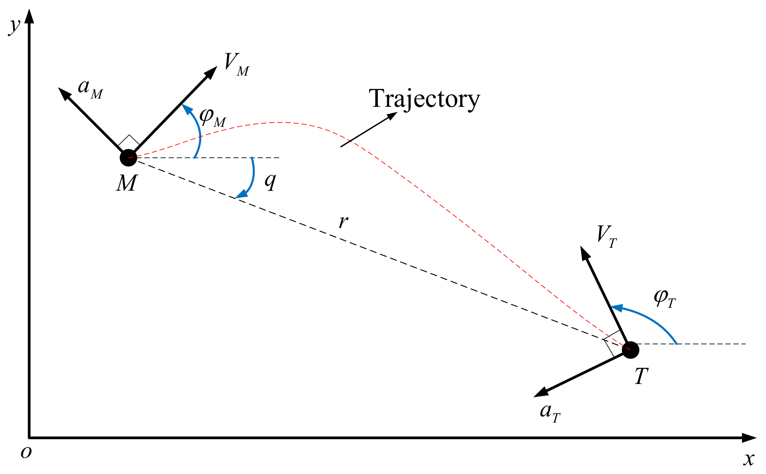
In this section, the proposed fractional-order control method is used as a guidance law for the interception of a missile with a target under an impact angle constraint. The planar missile–target engagement is shown in Figure 1. In the inertial coordinate system, the kinematic equations of the missile and target are expressed as follows [37,38]:

$$\left\{\begin{array}{c}{\dot{x}}_m=V_{m}cos\left({\phi }_m\right)\hfill \\ {\dot{y}}_m=V_{m}sin\left({\phi }_m\right)\hfill \\ {\dot{x}}_t=V_{t}cos\left({\phi }_t\right)\hfill \\ {\dot{y}}_t=V_{t}sin\left({\phi }_t\right)\hfill \\ {\dot{\phi }}_m=a_m/V_m\hfill \\ {\dot{\phi }}_t=a_t/V_t,\hfill \end{array}\right.$$

(62)

where r and $\dot{r}$ are the relative distance to the missile and the relative velocity of the target, respectively; ${\phi }_t$ denotes the aspect angle of the target; ${\phi }_m$ is the heading angle of the missile; and $V_m$ and $V_t$ are the velocities of the missile and target, respectively. We assume that $V_m$ and $V_t$ are constants. $a_m$ and $a_t$ denote the accelerations of the missile and target, respectively.

The kinematic equations of the missile and target in the rotating coordinate system are

$$\begin{array}{cc}\hfill \dot{r}& =V_{t}cos({\phi }_t-q)-V_{m}cos({\phi }_m-q),\hfill \end{array}$$

(63)

$$\begin{array}{cc}\hfill r\dot{q}& =V_{t}sin({\phi }_t-q)-V_{m}sin({\phi }_m-q),\hfill \end{array}$$

(64)

$$\begin{array}{cc}\hfill {\dot{\phi }}_t& =a_t/V_t,\hfill \end{array}$$

(65)

$$\begin{array}{cc}\hfill {\dot{\phi }}_m& =a_m/V_m,\hfill \end{array}$$

(66)

where q is the line of sight (LOS) angle and $\dot{q}$ is the LOS angular rate of the missile.

By differentiating Equation (64) with respect to time t and using Equations (63), (65), and (66), we obtain

$$\ddot{q}=-\frac{2\dot{r}}{r}\dot{q}-\frac{cos\left(q-{\phi }_m\right)}{r}{a}_m+\frac{cos\left(q-{\phi }_t\right)}{r}{a}_t.$$

(67)

In this study, required data such as q, $\dot{q}$, r, $\dot{r}$, and ${\varphi }_m$ were available. Let $q_d$ be the desired terminal LOS angle which is prespecified with a constant value. Let $q_e$ be the LOS angle error, that is, $q_e=q-q_d$. Define $x_1=q_e=q-q_d$ and $x_2=\dot{q}$. The missile acceleration $a_m$ can be regarded as a control variable, that is, $u=a_m$. Substituting these values into Equation (67) yields

$$\begin{array}{cc}\hfill {\dot{x}}_1& =x_2,\hfill \end{array}$$

(68)

$$\begin{array}{cc}\hfill {\dot{x}}_2& =-\frac{2\dot{r}}{r}{x}_2-\frac{cos(q-{\varphi }_m)}{r}u+\frac{cos(q-{\varphi }_t)}{r}{a}_t.\hfill \end{array}$$

(69)

Hence, Equations (68) and (69) can be expressed in the form of the nonlinear system (24) by writing the parameters as follows:

$$g=-\frac{2\dot{r}}{r}{x}_2,b=-\frac{cos\left(q-{\phi }_m\right)}{r},d=\frac{cos\left(q-{\phi }_t\right)}{r}{a}_t.$$

To verify the validity of the proposed guidance law, simulations were performed with three different target accelerations, which were as follows [39]:

Case 1:$a_T=7 \mathrm{g}cos(\pi t/4)\mathrm{m}/{\mathrm{s}}^2$.

Case 2:$a_T=7 \mathrm{g}\mathrm{m}/{\mathrm{s}}^2$ for $t<5\mathrm{s}$ and $a_T=-7 \mathrm{g}\mathrm{m}/{\mathrm{s}}^2$ for $t\ge 5\mathrm{s}$.

Case 3:$a_T=7 \mathrm{g}\mathrm{m}/{\mathrm{s}}^2$.

In the following subsection, the effectiveness of the proposed fractional-order sliding mode guidance law (61) is verified through a series of simulations. First, simulations with different fractional orders in the three cases are presented to illustrate the influence of the fractional order on the guidance results. Simulations with $\alpha =0$ are given specifically for comparison with the fractional-order method. Subsequently, a comparison of the proposed guidance law and the fractional guidance law in Ref. [15] exhibits the advantages of the proposed guidance law. Finally, simulations are performed with different desired terminal LOS angles to demonstrate the performance of the proposed method in satisfying the impact angle constraints.

3.1. Simulation Results with Different Fractional Orders

In this subsection, the simulations with the proposed guidance law (61) under different fractional orders are described. The parameters of the proposed guidance law were as follows: $a_1=0.5$, $a_2=0.5$, $a_3=2/3$, ${\rho }_1=1.1$, ${\rho }_2=2$, ${\rho }_3=6$, $\sigma =1.1$, and $\delta =0.002$. Additional constants and initial values are listed in

Table 1. Some constants and initial conditions for the missile and the target in the simulations with differential fractional orders.

Parameter	Data	Parameter	Data
$x_m\left(0\right)$	0 m	$x_t\left(0\right)$	2500$\sqrt{3}$ m
$y_m\left(0\right)$	0 m	$y_t\left(0\right)$	2500 m
$V_m$	600 m/s	$V_t$	300 m/s
${\varphi }_m\left(0\right)$	60${}^{\circ }$	${\varphi }_t\left(0\right)$	0${}^{\circ }$

. The impact angle constraint was 20${}^{\circ }$. The maximum acceleration of the missile was set to 40 $\mathrm{g}$, where $\mathrm{g}=9.8 \mathrm{m}/{\mathrm{s}}^2$ was the acceleration owing to gravity.

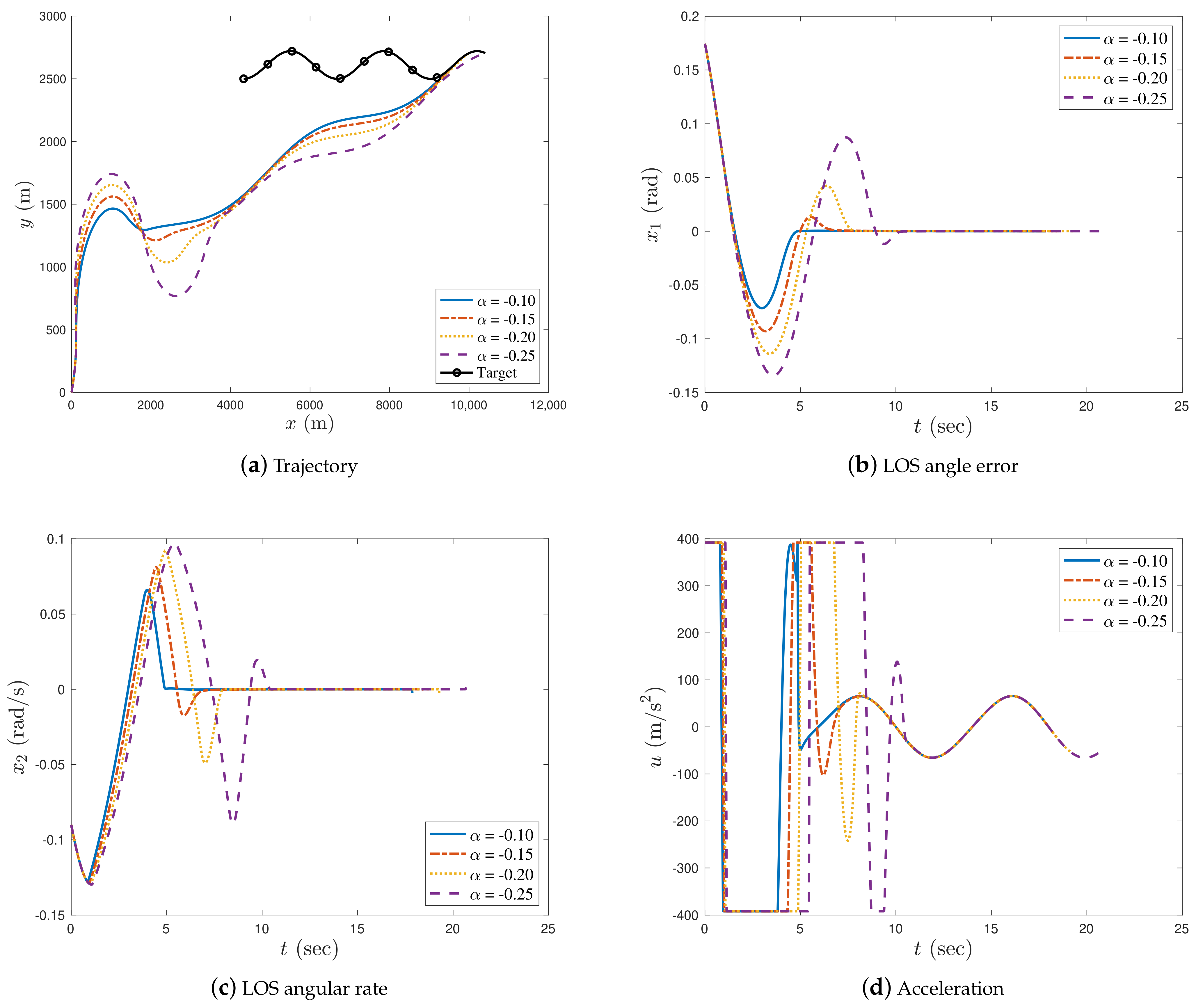
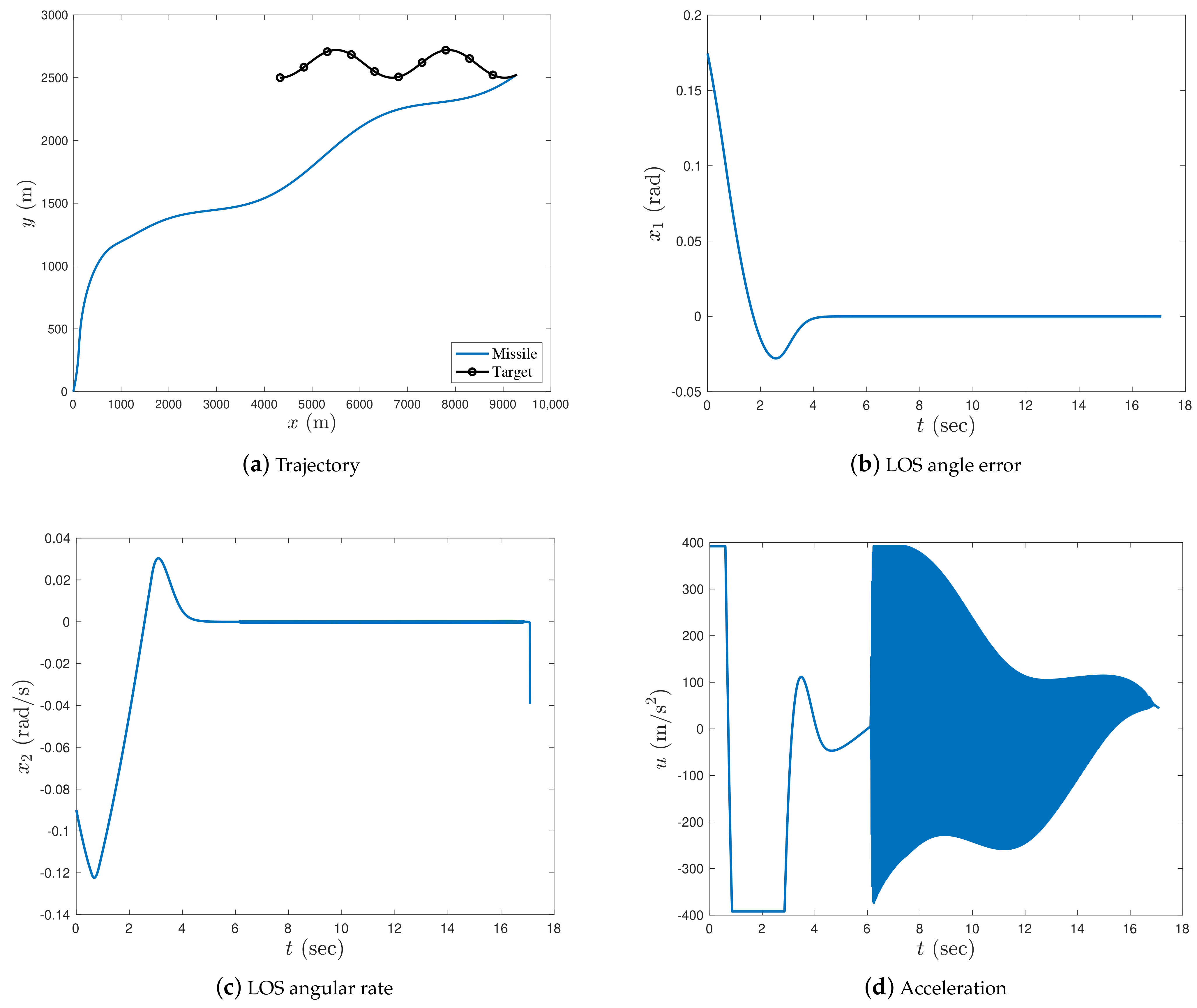
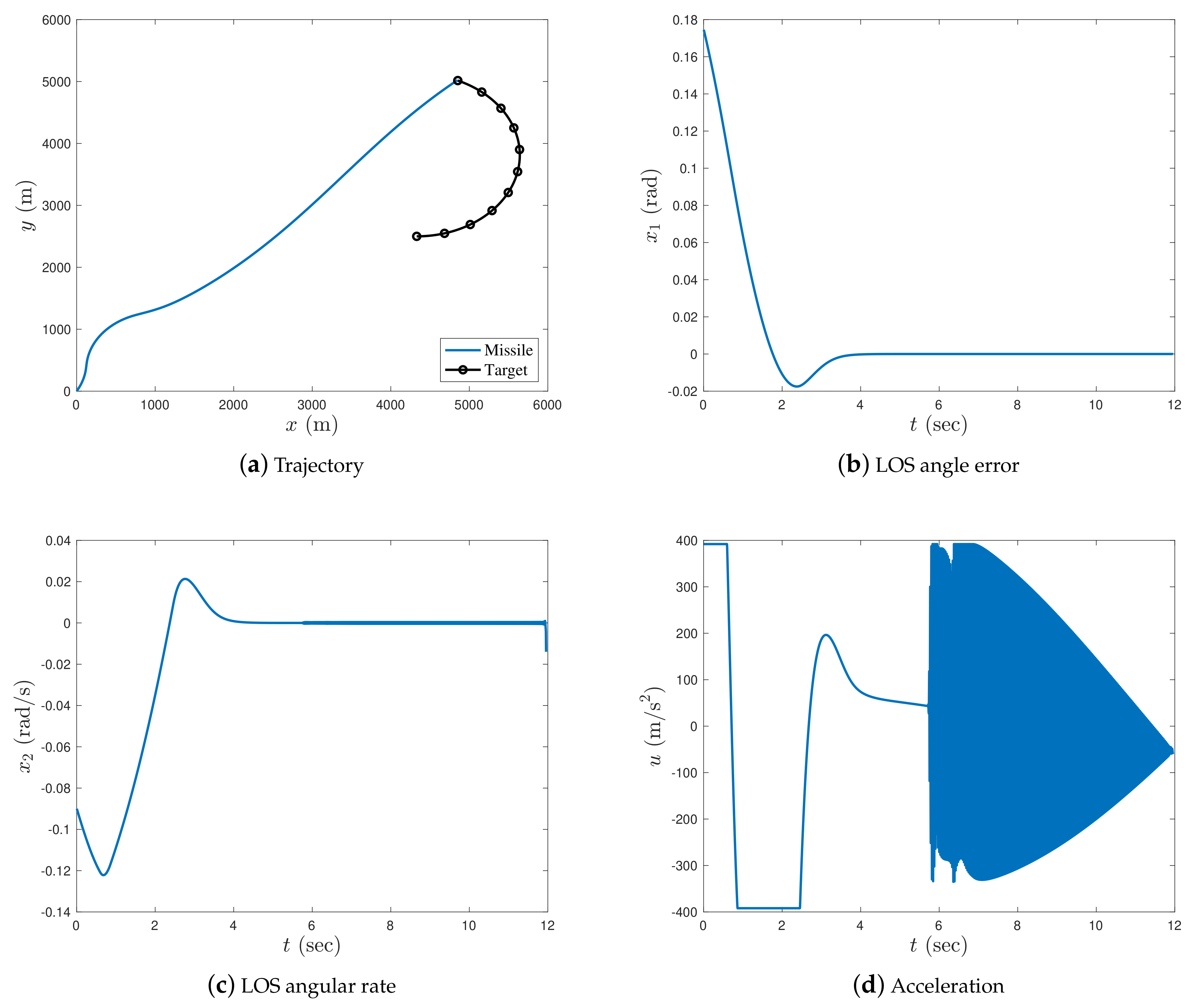
Figure 2 and Figure 3 show the simulation results with the fractional differential ($\alpha >0$) and fractional integral ($\alpha <0$) guidance laws, respectively, in case 1. Figure 4 shows the simulation results with the integer ($\alpha =0$) guidance law for case 1. Interception times, miss distances and LOS angle errors of the proposed guidance law under all chosen fractional orders in case 1 are shown in

Table 2. Interception times, miss distances, and LOS angle errors of the proposed guidance laws under different fractional orders in case 1.

Fractional Order	Interception Time (s)	Miss Distance (m)	LOS Angle Error (rad)
−0.25	18.426	0.016	6.671 × 10${}^{-5}$
−0.20	18.426	0.013	4.090 × 10${}^{-5}$
−0.15	18.426	0.013	2.293 × 10${}^{-5}$
−0.10	17.866	0.012	3.180 × 10${}^{-6}$
0	16.870	0.010	1.680 × 10${}^{-6}$
0.1	16.521	0.012	1.000 × 10${}^{-4}$
0.3	16.111	0.013	2.700 × 10${}^{-3}$
0.6	16.111	0.014	2.650 × 10${}^{-2}$
0.8	16.111	0.079	6.400 × 10${}^{-2}$

. Figure 5, Figure 6 and Figure 7 show the simulation results with fractional differential, fractional integral, and integer-order guidance laws, respectively, in case 2. Interception times, miss distances and LOS angle errors of the proposed guidance law under all selected fractional orders in case 2 are shown in

Table 3. Interception times, miss distances, and LOS angle errors of the proposed guidance laws under different fractional orders in case 2.

Fractional Order	Interception Time (s)	Miss Distance (m)	LOS Angle Error (rad)
−0.25	15.957	0.021	9.300 × 10${}^{-6}$
−0.20	15.957	0.018	2.503 × 10${}^{-6}$
−0.15	15.957	0.016	7.836 × 10${}^{-7}$
−0.10	15.798	0.005	1.895 × 10${}^{-7}$
0	15.474	0.002	1.094 × 10${}^{-7}$
0.1	15.328	0.037	1.000 × 10${}^{-4}$
0.3	15.169	0.081	1.438 × 10${}^{-4}$
0.6	15.169	0.019	2.900 × 10${}^{-3}$
0.8	15.169	0.029	2.740 × 10${}^{-2}$

, Figure 8 and Figure 9 show the simulation results with $\alpha >0$ and $\alpha <0$ in case 3, and Figure 10 depicts the simulation results with the integer-order guidance law in case 3. Interception times, miss distances, and the LOS angle errors of the proposed guidance law under all selected fractional orders in case 3 are shown in

Table 4. Interception times, miss distances, and LOS angle errors of the proposed guidance laws under different fractional orders in case 3.

Fractional Order	Interception Time (s)	Miss Distance (m)	LOS Angle Error (rad)
−0.25	12.626	0.046	6.793 × 10${}^{-6}$
−0.20	12.386	0.020	2.349 × 10${}^{-6}$
−0.15	12.227	0.017	7.813 × 10${}^{-7}$
−0.10	12.113	0.015	1.167 × 10${}^{-7}$
0	11.889	0.010	1.065 × 10${}^{-7}$
0.1	11.792	0.012	2.165 × 10${}^{-4}$
0.3	11.709	0.018	4.000 × 10${}^{-3}$
0.6	11.740	0.035	3.190 × 10${}^{-2}$
0.8	11.788	0.058	6.190 × 10${}^{-2}$

.

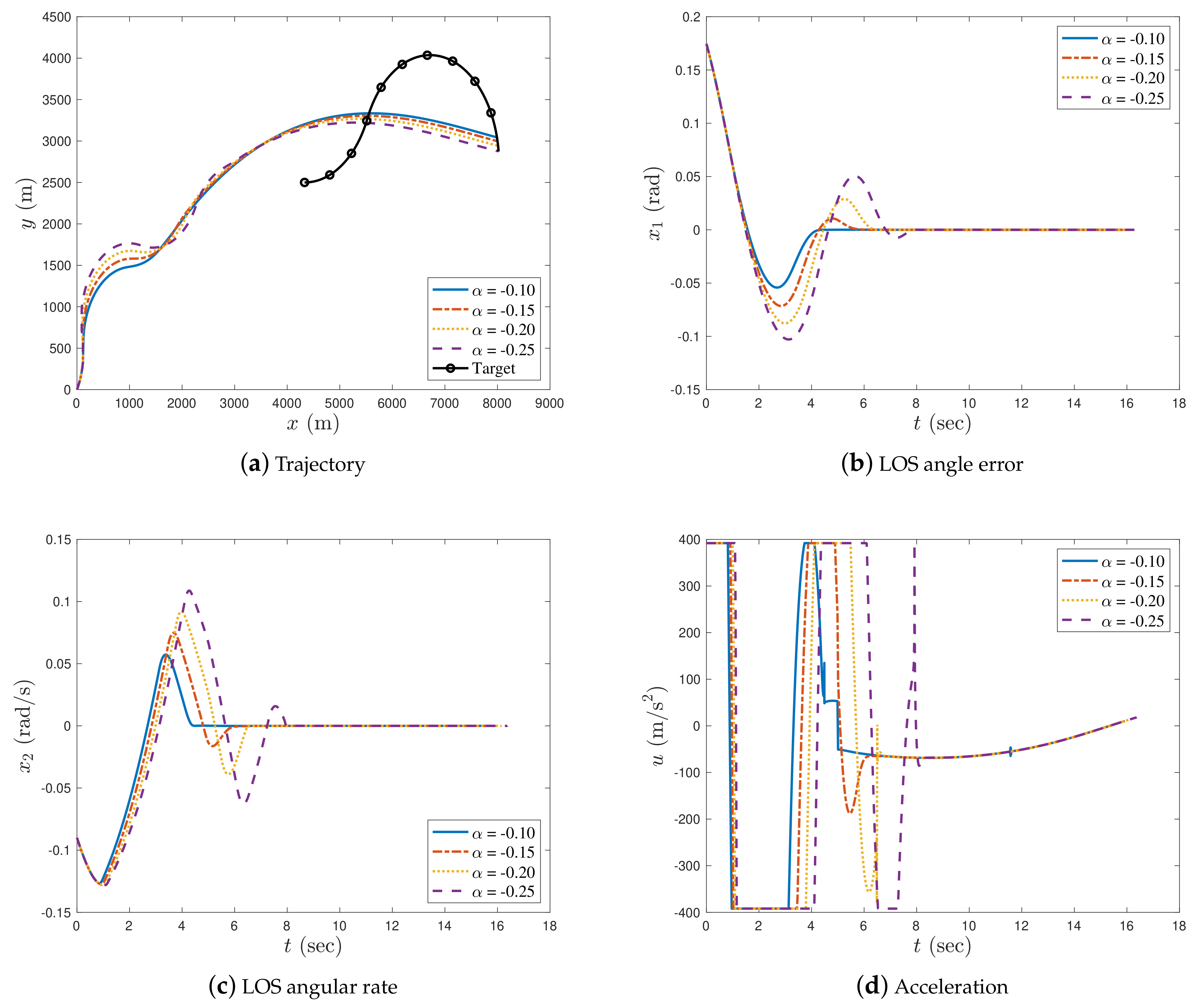
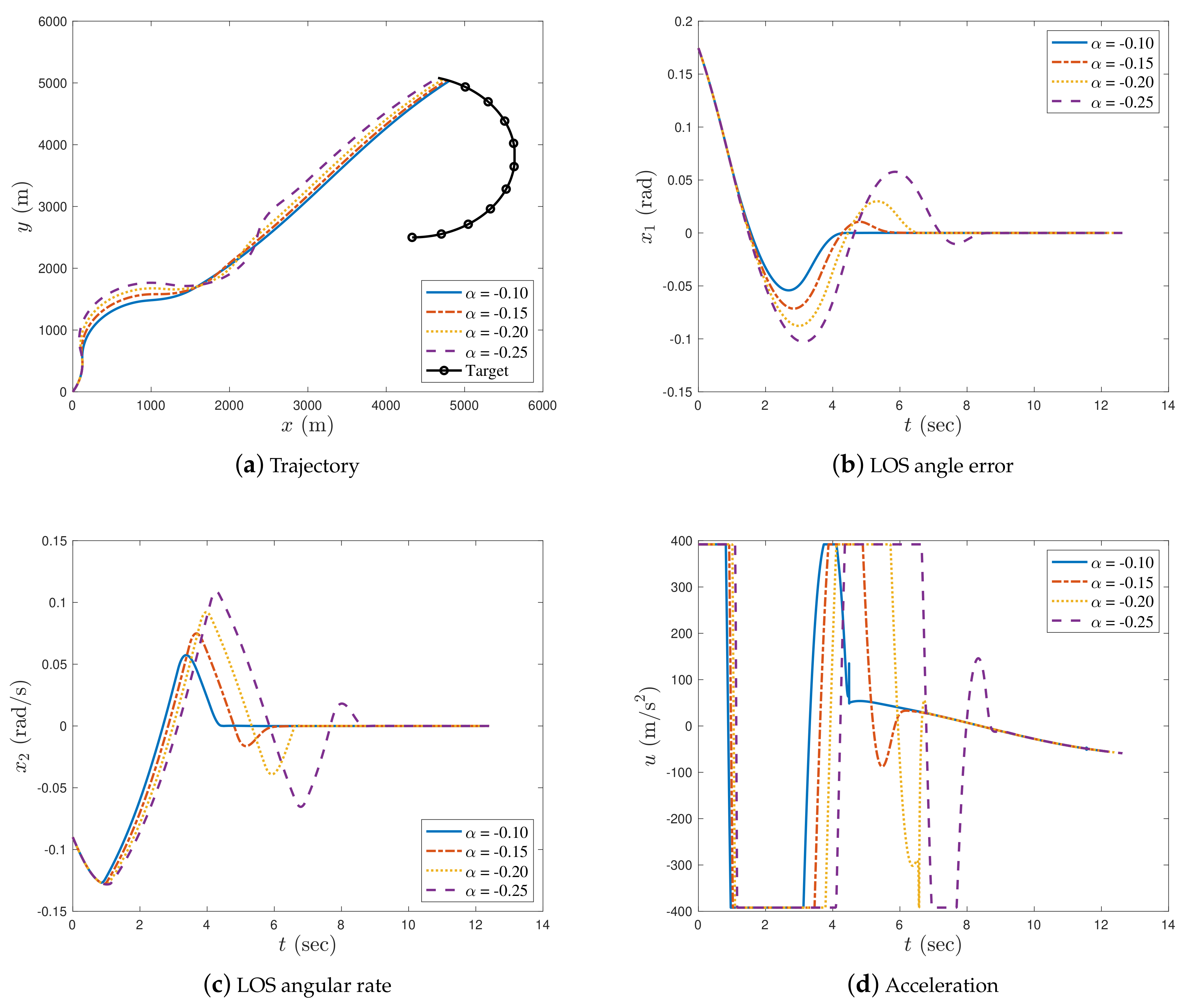
In case 1, as illustrated in Figure 2a, Figure 3a, and Figure 4a, the missile successfully intercepted the manoeuvring target under all given fractional orders. As can be seen in Figure 2b, when $\alpha >0$, the LOS angle error increased with an increase in α; therefore, the LOS angle error was asymptotically stable and the impact angle constraint of the missile could not be satisfied when α was relatively large. Thus, we set α sufficiently small to ensure the convergence of the LOS angle error during the interception process. When $\alpha <0$, the LOS angle error asymptotically converged to zero, and the smaller the value of α, the larger the oscillation of the LOS angle error (see Figure 3b). In Figure 4b, the LOS angle error converges to zero in finite time when $\alpha =0$. From Figure 2c, Figure 3c, and Figure 4c, it can be observed that the LOS angular rate of the missile converges to zero for all values of α. In Figure 2c and Figure 3c, the LOS angular rate is asymptotically stable, whereas that in Figure 4c is finite-time stable. In addition, it was observed that the closer the order of α was to zero (either to the right or left), the faster the convergence speed of the missile’s LOS angular rate.

It can be noted from Table 2 that the interception times taken by the proposed guidance law with $\alpha >0$ were similar, while the interception time was longer with the decrease in fractional order when $\alpha <0$. It can also be observed that the miss distance and the LOS angle error were smaller when the fractional order of the proposed guidance law approached zero.

In Figure 2d and Figure 3d, the acceleration of the missile is smooth and steady for both the fractional differential and fractional integral guidance laws. However, as illustrated in Figure 4d, the acceleration trajectory of the missile with the integer-order guidance law chattered after approximately 7 s. This is because the proposed guidance law contains a singular term when $\alpha =0$. Figure 2d and Figure 3d show that the fractional-order differential and integral guidance laws were effective in eliminating the chattering caused by singular terms.

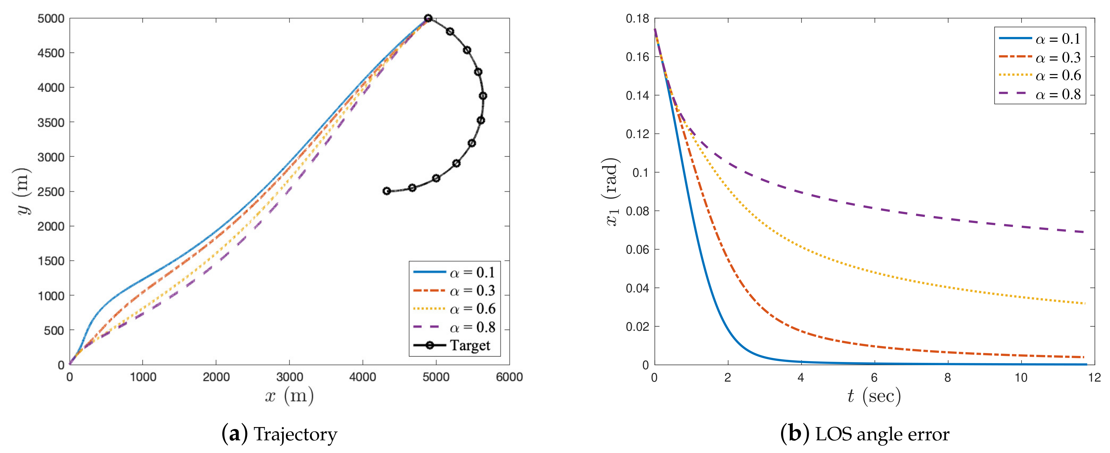
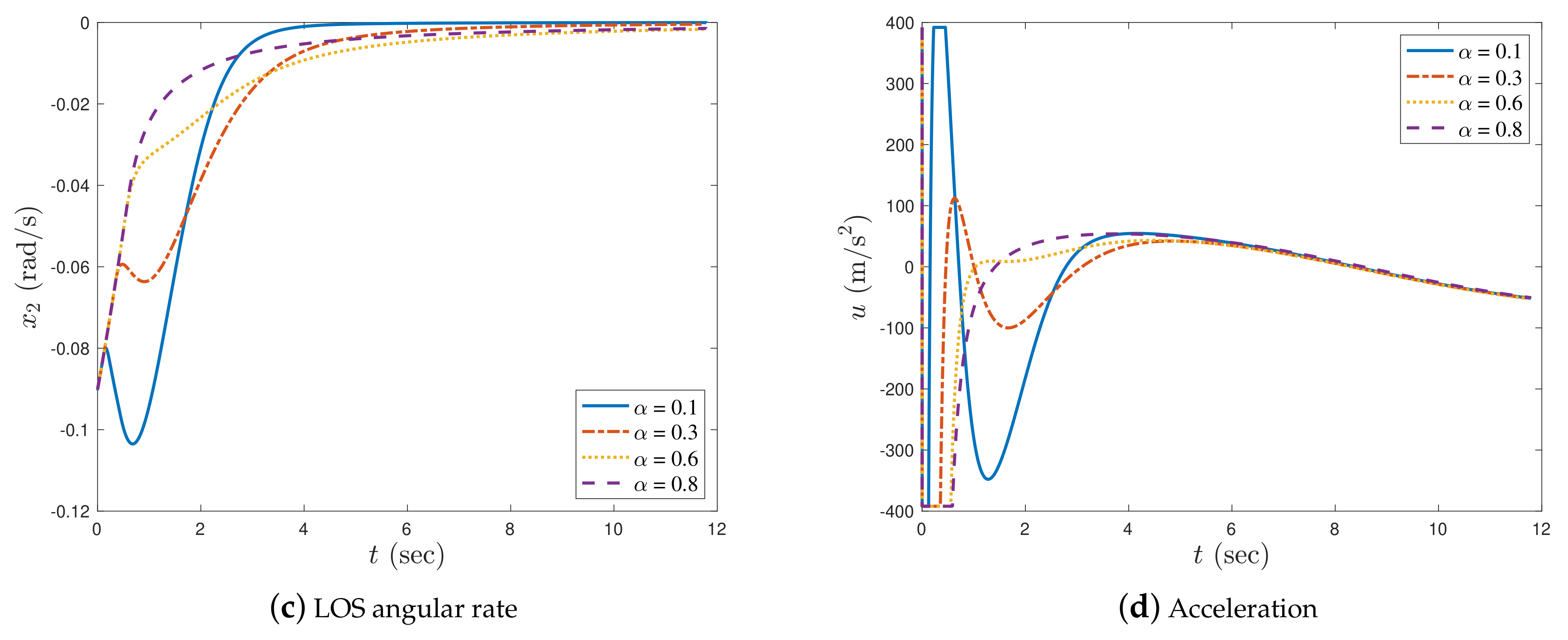
In case 2, Figure 5, Figure 6 and Figure 7 show the simulation results under $\alpha >0$, $\alpha <0$, and $\alpha =0$, respectively. As shown in Figure 5a, Figure 6a, and Figure 7a, the missile achieved an accurate interception of the manoeuvring target for all different fractional orders. The impact time decreased when the fractional order approached zero (either from the left or right). From Figure 5b, Figure 6b, and Figure 7b, it can be seen that the missile’s LOS angle error converged in the neighbourhood of zero when the fractional order was close to zero: the convergence time was shorter with smaller fractional orders. When α was far from zero, the LOS angle error did not converge to zero during the interception process; therefore, the impact angle constraint was not satisfied. In Figure 5c, Figure 6c, and Figure 7c, it can be seen that the missile’s LOS angular rate converged to zero during the interception process.

It can be noted from Table 3 that the interception times taken by the proposed guidance law with $\alpha >0$ were similar, while the interception time was longer with the decrease in fractional order when $\alpha <0$. It can also be observed that the miss distance and the LOS angle error were smaller when the fractional order of the proposed guidance law approached zero.

In Figure 5d and Figure 6d, as in case 1, the acceleration of the missile is smooth and steady for both $\alpha >0$ and $\alpha <0$; however, the acceleration trajectory of the missile for $\alpha =0$ also chattered after approximately 7 s (see Figure 7d) due to the proposed guidance law containing a singular term when $\alpha =0$. Figure 5d and Figure 6d show that the fractional-order differential and integral guidance laws were effective in eliminating the chattering caused by the singular terms. In Figure 6d, the acceleration of the missile with $\alpha =-0.1$ had a small chatter at 12 s. Compared to the missile acceleration when $\alpha =0$ in Figure 7d, the chattering is so small that it can be ignored. Thus, it can be concluded that the proposed fractional-order method is effective for eliminating chattering.

The simulation results for case 3 are shown in Figure 8, Figure 9 and Figure 10 and Table 4, from which it can be seen that the results were similar to those in cases 1 and 2; therefore, discussions on this case are omitted.

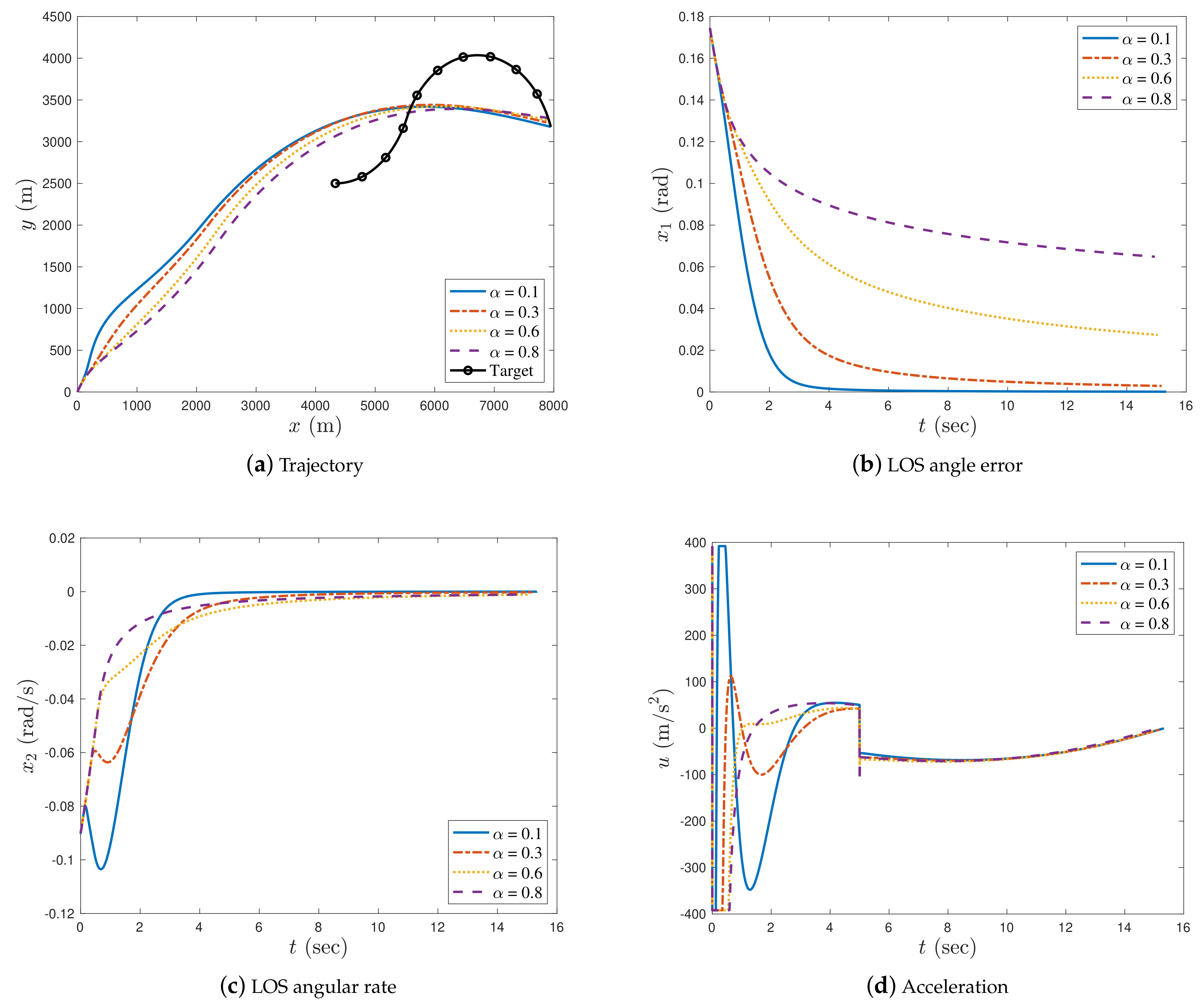
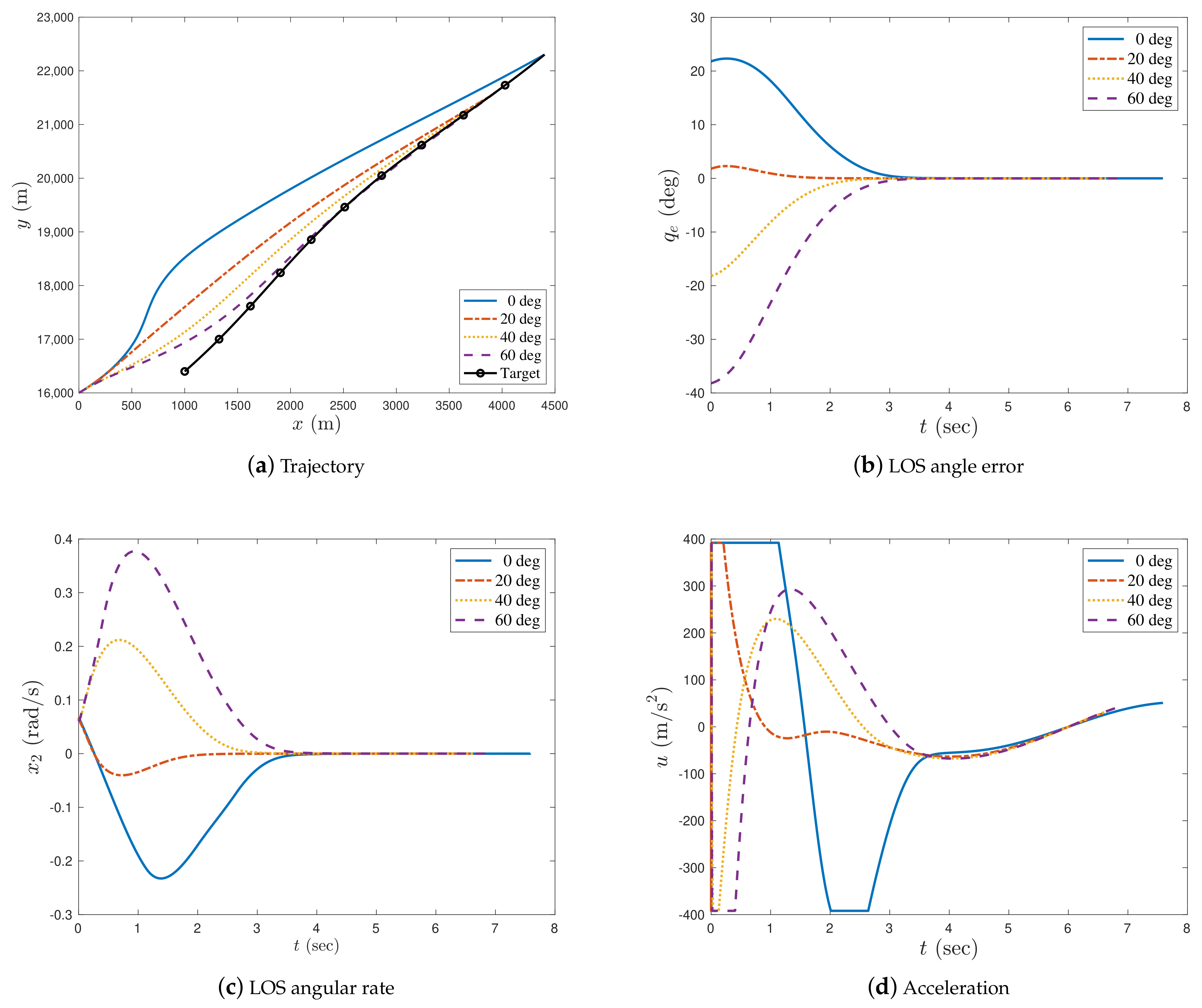
3.2. Simulations with Different Impact Angle Constraints

In this subsection, simulations with different desired terminal LOS angles but the same initial flight path angles as those of the previous subsection are described. These simulations were carried out to verify the proposed fractional-order guidance law with different impact angle constraints. The initial conditions of the missile and target are listed in

Table 5. Some constants and initial conditions for the missile and the target in the simulations with different terminal LOS angles.

Parameter	Data	Parameter	Data
$x_m\left(0\right)$	0 m	$x_t\left(0\right)$	1000 m
$y_m\left(0\right)$	16,000 m	$y_t\left(0\right)$	16,400 m
$V_m$	$1032.7$ m/s	$V_t$	900 m/s
${\varphi }_m\left(0\right)$	50${}^{\circ }$	${\varphi }_t\left(0\right)$	60${}^{\circ }$

. The desired terminal LOS angles were 0${}^{\circ }$, 20${}^{\circ }$, 40${}^{\circ }$, and 60${}^{\circ }$. The target acceleration was chosen as $a_t=7\mathrm{g}cos(\pi t/4)\mathrm{m}/{\mathrm{s}}^2$. The fractional order was set to $\alpha =0.01$. Using the proposed guidance law, the trajectories of the missile and target, the missile LOS angle error, LOS angular rate, and acceleration were as shown in Figure 11.

From Figure 11a, we can observe that the missile successfully intercepted the manoeuvring target at different impact angles. Figure 11b,c show that when $q_d=0^{\circ },{20}^{\circ },{40}^{\circ }$, or ${60}^{\circ }$, the LOS angle errors and LOS angular rates were asymptotically stable. From Figure 11d we can observe that the accelerations of the missile were within reasonable bounds, and there was no chattering during the interception process with different terminal LOS angles. Therefore, the fractional guidance law is very effective in eliminating chattering. The only disadvantage is that when using fractional derivative or integral guidance laws, the LOS angle error and LOS angular rate converge to zero asymptotically rather than in finite time. However, the value of α near zero can be adjusted continuously such that the LOS angle error and LOS angular rate can achieve satisfactory convergence.

3.3. Simulation for Comparison with Different Method

In this subsection, simulations for comparison between the guidance law proposed in this study and the guidance law in Ref. [15] are presented.

The fractional-order sliding surface proposed by Sheng et al. [15] is expressed as

$$s=x_2+c_1{x}_1+c_2{D}^{\alpha }\left(x_1+x_2\right),$$

(70)

where $c_1,c_2>0$ and α is non-zero. The corresponding fractional sliding mode-based guidance law is

$$u=-\frac{1}{b}\left[g+c_1{x}_2+c_2{D}_t^{1+\alpha }(x_1+x_2)+P\mathrm{sgn}\left(s\right)\right],$$

(71)

where P denotes a positive constant.

It is simple to prove that the sliding surface $s\left(t\right)$ converges to zero in finite time. Thus, there exists $t_1$ such that for all $t\ge t_1$, the sliding surface satisfies $s\left(t\right)\equiv 0$. Therefore, Equation (70) can be represented as:

$${\dot{x}}_1=-c_1{x}_1-c_2{D}^{\alpha }(x_1+x_2).$$

(72)

Without loss of generalisation, we assume $\alpha >0$ to obtain

$$\frac{\mathrm{d}}{\mathrm{d}t}{x}_1=-c_1{x}_1-c_2\frac{\mathrm{d}}{\mathrm{d}t}\left[J^{1-\alpha }(x_1+x_2)\right].$$

(73)

Integrating both sides of Equation (73) from $t_0$ to t yields:

$$x_1\left(t\right)=-c_1{\int }_{t_0}^t{x}_1\left(\tau \right)\mathrm{d}\tau -c_2{J}^{1-\alpha }(x_1+x_2)\left(t\right)+C,$$

(74)

where C is a constant. Taking the fractional derivative of order $(1-\alpha )$ in the Caputo sense on both sides of Equation (74) yields

$$\begin{array}{cc}\hfill {}_{t_0}^{\mathrm{C}}{D}_t^{1-\alpha }{x}_1\left(t\right)& =-c_1{}_{t_0}^{\mathrm{C}}{D}_t^{1-\alpha }{J}^1{x}_1\left(t\right)-c_2(x_1+x_2)\hfill \\ \hfill & =-c_1{J}^{\alpha }{D}^1{J}^1{x}_1\left(t\right)-c_2(x_1+x_2)\hfill \\ \hfill & =-c_1{J}^{\alpha }{x}_1\left(t\right)-c_2{x}_1-c_2{x}_2.\hfill \end{array}$$

(75)

We cannot explicitly determine the convergence of $x_1$. In Ref. [15], the authors set $c_2$ to be extremely small ($c_2={10}^{-5}$) so that the fractional-order term in Equation (70) can be regarded as a small perturbation. Thus, only the stability of the system ${\dot{x}}_1=-c_1{x}_1$ must be examined. It is easy to see that the zero solution of system ${\dot{x}}_1=-c_1{x}_1$ is exponentially stable, and systems with small perturbations ${\dot{x}}_1=-c_1{x}_1+d$ are also stable.

In the simulations, the parameters of the proposed guidance law were $a_1=0.5$, $a_2=0.5$, $a_3=2/3$, ${\rho }_1=1.1$, ${\rho }_2=2$, ${\rho }_3=6$, $\sigma =1.1$, and $\sigma =0.002$, and the parameters of the guidance law in Ref. [15] were $c_1=1/2$, $c_2=0.1$, and $P=0.3$. The terminal LOS angle was $q_d={20}^{\circ }$. The target acceleration was chosen as $a_t=7\mathrm{g}cos(\pi t/4)\mathrm{m}/{\mathrm{s}}^2$. 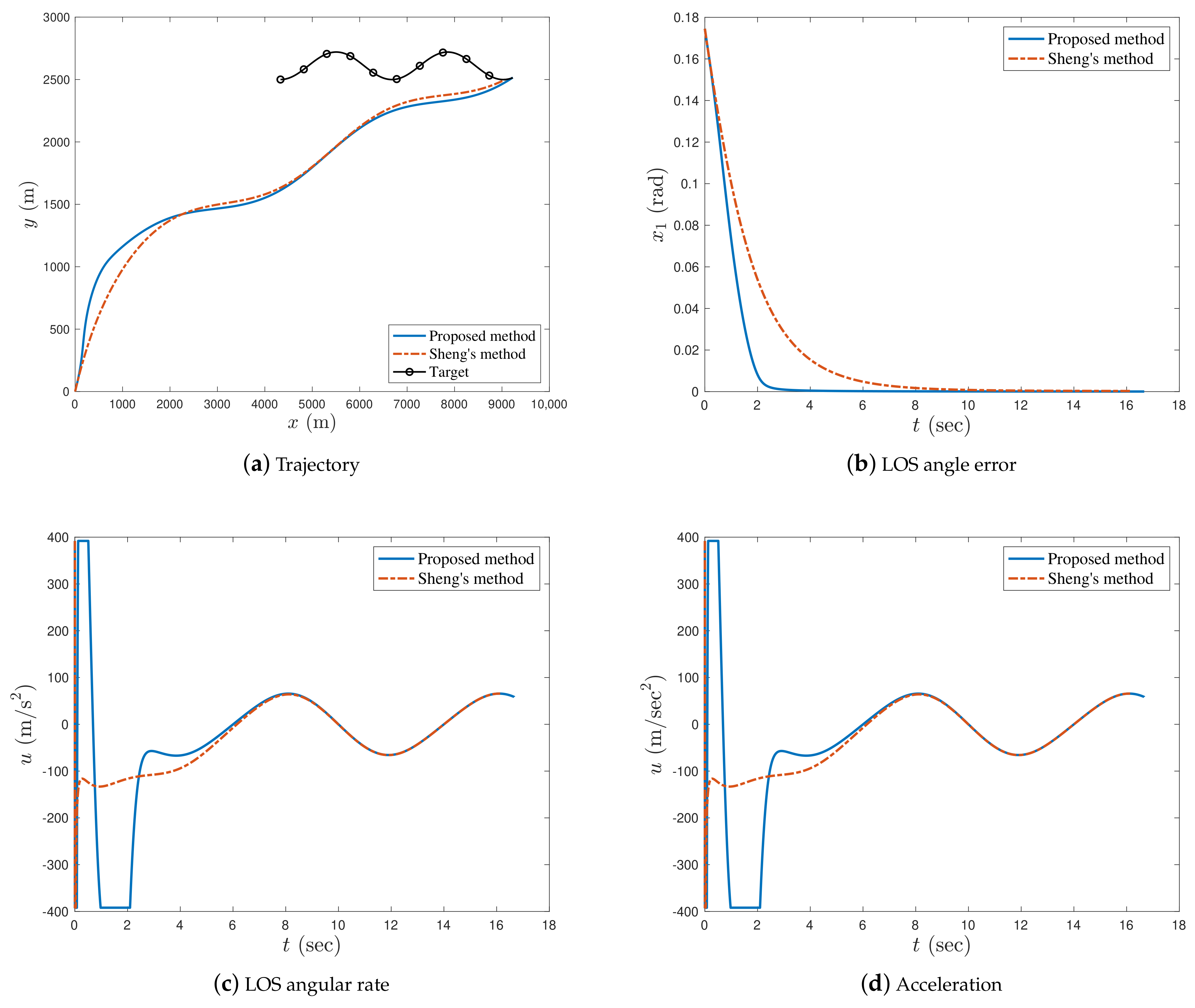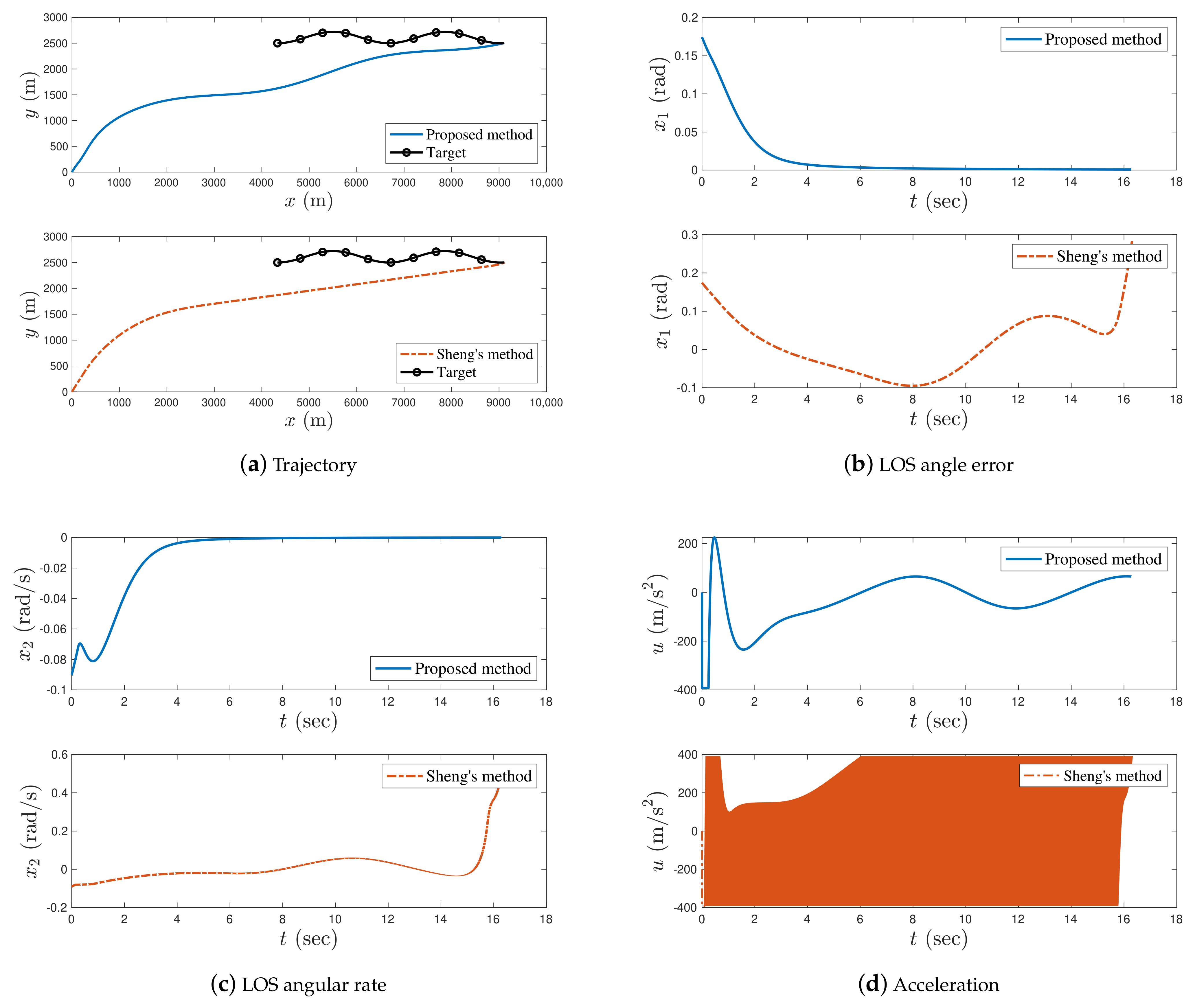The initial conditions and additional constants are listed in Table 5. To investigate the efficiency of the proposed method, simulations were performed with $\alpha =0.007$ and $\alpha =0.3$ separately, and the results are shown in Figure 12 and Figure 13. The interception times, the miss distance, and the LOS angle errors are shown in

Table 6. Interception times, miss distances, and LOS angle errors of two guidance laws with $\alpha =0.07$.

Guidance Law	Interception Time (s)	Miss Distance (m)	LOS Angle Error (rad)
Sheng’s method	16.668	0.224	3.328 × 10${}^{-4}$
Proposed method	16.133	0.043	2.879 × 10${}^{-5}$

and

Table 7. Interception times, miss distances, and LOS angle errors of two guidance laws with $\alpha =0.3$.

Guidance Law	Interception Time (s)	Miss Distance (m)	LOS Angle Error (rad)
Sheng’s method	16.304	0.278	0.283
Proposed method	16.278	0.200	7.893 × 10${}^{-4}$

.

When $\alpha =0.07$, the proposed fractional-order guidance law and the fractional-order guidance law from Ref. [15] successfully intercepted a target (see Figure 12a). The convergence speed of the LOS angle error and LOS angular rate with the proposed guidance law were faster than those with the guidance law from Ref. [15]. As shown in Figure 12d, the accelerations of the missiles with the proposed guidance law and guidance law in Ref. [15] were all within a reasonable scope, but there was acceleration saturation when using the proposed method to achieve faster convergence.

From Table 6, the missile distance and the LOS angle error of the proposed guidance law were smaller than those of Sheng’s method. Thus, the guidance precision of the proposed guidance law was significantly superior to that of Sheng’s method.

When $\alpha =0.3$, Figure 13a,c show that the LOS angle error and LOS angular rate with the proposed guidance law were asymptotically stable during the interception process, whereas the LOS angle error and LOS angular rate with the guidance law from Ref. [15] were unstable. It can be observed in Figure 13d that the acceleration of the missile with the proposed guidance law was within a reasonable scope without any chattering, whereas the acceleration of the missile with the guidance law in Ref. [15] demonstrated high-frequency chattering in the acceleration bound. The simulation results indicated that the proposed guidance law had better robustness and a larger stability region than the guidance law in Ref. [15].

From Table 7, the missile distance of the proposed guidance law was smaller than that of Sheng’s method. It can be observed that the LOS angle error of Sheng’s method cannot ensure the terminal LOS angle constraint, while the LOS angle error of the proposed method was within a reasonable range. Thus, the guidance precision of the proposed guidance law is significantly superior to that of Sheng’s method.

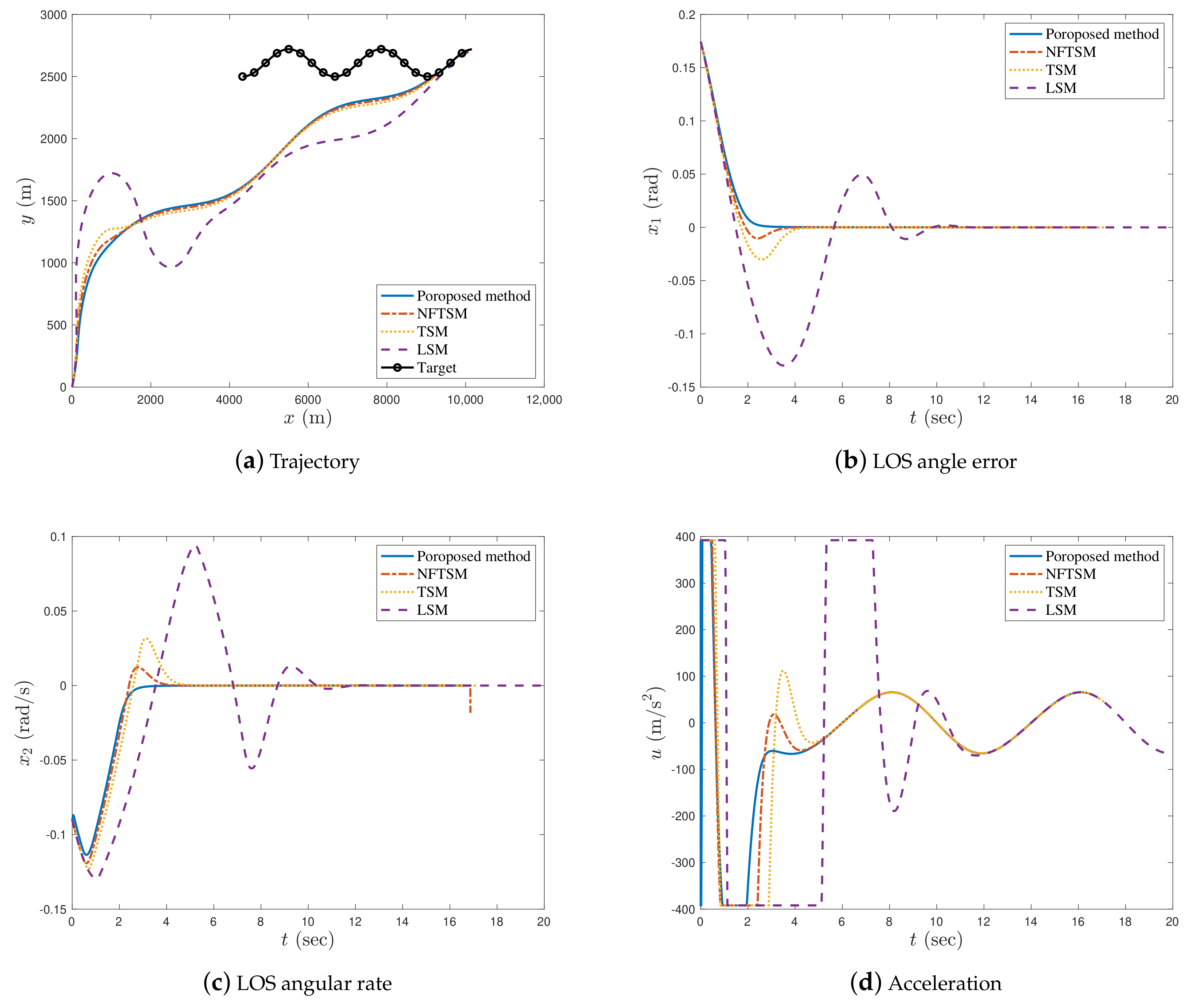
The next set of simulations for the guidance laws based on the integer-order linear sliding mode (LSM) [39], terminal sliding mode (TSM) [39], and nonsingular fast terminal sliding mode (NFTSM) [39] are shown for the comparison with the presented guidance law in this paper. All parameters of the LSM, TSM, and NFTSM guidance laws are the same as those chosen in the presented guidance law. The initial conditions of the missile and the target, the terminal LOS angle, and the target acceleration are the same as those of the previous simulation in this subsection. The fractional order of the proposed guidance law is set to 0.03. The trajectories of the missile and the target, the LOS angle, the LOS angular rate, and the missile acceleration for the four guidance laws are shown in Figure 14.

As shown in Figure 14a, it can be seen that the proposed fractional-order guidance law and the other three guidance laws based on integer-order sliding mode successfully intercepted a target. The convergence speed of the LOS angle error and LOS angular rate with the proposed guidance law were faster than those with the guidance laws based on integer-order sliding mode. As shown in Figure 14d, the accelerations of the missiles with the proposed guidance law and guidance laws based on integer sliding mode were all within a reasonable scope, but there was acceleration saturation when using the proposed method to achieve faster convergence.

From

Table 8. Interception times, miss distances, and LOS angle errors of different guidance laws.

Guidance Law	Interception Time (s)	Miss Distance (m)	LOS Angle Error (rad)
Proposed method	16.687	0.034	2.336 × 10${}^{-5}$
NFTSM	16.870	0.149	1.680 × 10${}^{-6}$
TSM	17.126	0.048	1.550 × 10${}^{-6}$
LSM	19.857	0.073	7.190 × 10${}^{-6}$

, it is clear that the interception time taken by the proposed guidance law and the NFTSM guidance law is similar. However, the LSM guidance law has a longer interception time than the other guidance laws. The miss distance of the proposed guidance law is smaller than the other guidance laws. However, the LOS angle error generated by the proposed guidance law is bigger than that of the other integer-order guidance laws. This is because the proposed guidance law can only ensure asymptotic convergence rather than the finite-time convergence.

4. Conclusions

In this study, a useful fractional-order stability theorem was established, which can be utilized as a fractional-order Lyapunov direct method. Subsequently, a novel fractional-order sliding surface was proposed, and a fractional-order sliding mode-based control law for a class of integer-order nonlinear systems was designed. The advantage of the method in this study is that it allows for the use of FO-SMC for a class of integer-order nonlinear systems, rather than fractional systems, which makes the method possible in practical applications. Furthermore, the stability property of the controlled system was proven by the proposed Lyapunov theorem, which simplified the proof process. The only disadvantage is that with the FO-SMC law, the nonlinear system can only guarantee asymptotic stability. However, this disadvantage can be overcome by adjusting the fractional order using trial and error. By using the proposed method in an example of the missile–target interception problem with impact angle constraints, it was shown that the proposed method can guarantee convergence of the LOS angle and LOS angular rate to zero, thus demonstrating the effectiveness of the method.

References

1. Bagley, R.L.; Torvik, P.J. On the fractional calculus model of viscoelastic behavior. J. Rheol. 1986, 30, 133–155. [Google Scholar] [CrossRef]
2. Freed, A.; Diethelm, K. Fractional calculus in biomechanics: A 3D viscoelastic model using regularized fractional derivative kernels with application to the human calcaneal fat pad. Biomech. Model. Mechanobiol. 2006, 5, 203–215. [Google Scholar] [CrossRef] [PubMed]
3. Scalas, E.; Gorenflo, R.; Mainardi, F. Fractional calculus and continuous-time finance. Phys. A Stat. Mech. Appl. 2000, 284, 376–384. [Google Scholar] [CrossRef] [Green Version]
4. David, S.; Fischer, C.; Machado, J.T. Fractional electronic circuit simulation of a nonlinear macroeconomic model. AEU Int. J. Electron. Commun. 2018, 84, 210–220. [Google Scholar] [CrossRef]
5. Pan, B.; Fareed, U.; Qing, W.; Tian, S. A novel fractional order PID navigation guidance law by finite time stability approach. ISA Trans. 2019, 94, 80–92. [Google Scholar] [CrossRef] [PubMed]
6. Zamani, M.; Karimighartemani, M.; Sadati, N.; Parniani, M. Design of a fractional order PID controller for an AVR using particle swarm optimization. Control Eng. Pract. 2009, 17, 1380–1387. [Google Scholar] [CrossRef]
7. Padula, F.; Visioli, A. Advances in Robust Fractional Control; Springer: New York, NY, USA, 2015. [Google Scholar]
8. Podlubny, I. Fractional-order systems and fractional-order controllers. Inst. Exp. Phys. Slovak Acad. Sci. Kosice 1994, 12, 1–18. [Google Scholar]
9. Monje, C.A.; Vinagre, B.M.; Feliu, V.; Chen, Y. Tuning and auto-tuning of fractional order controllers for industry applications. Control Eng. Pract. 2008, 16, 798–812. [Google Scholar] [CrossRef] [Green Version]
10. Zheng, M.; Li, L.; Peng, H.; Xiao, J.; Yang, Y.; Zhao, H. Finite-time projective synchronization of memristor-based delay fractional-order neural networks. Nonlinear Dyn. 2017, 89, 2641–2655. [Google Scholar] [CrossRef]
11. Pourmahmood Aghababa, M. Robust Finite-Time Stabilization of Fractional-Order Chaotic Systems based on Fractional Lyapunov Stability Theory. J. Comput. Nonlinear Dyn. 2012, 7, 021010. [Google Scholar] [CrossRef]
12. Ding, Z.; Zeng, Z.; Wang, L. Robust finite-time stabilization of fractional-order neural networks with discontinuous and continuous activation functions under uncertainty. IEEE Trans. Neural Netw. Learn. Syst. 2017, 29, 1477–1490. [Google Scholar] [CrossRef] [PubMed]
13. Aghababa, M.P. A Lyapunov-based control scheme for robust stabilization of fractional chaotic systems. Nonlinear Dyn. 2014, 78, 2129–2140. [Google Scholar] [CrossRef]
14. Delavari, H.; Ghaderi, R.; Ranjbar, A.; Momani, S. Fuzzy fractional order sliding mode controller for nonlinear systems. Commun. Nonlinear Sci. Numer. Simul. 2010, 15, 963–978. [Google Scholar] [CrossRef]
15. Sheng, Y.; Zhang, Z.; Xia, L. Fractional-order sliding mode control based guidance law with impact angle constraint. Nonlinear Dyn. 2021, 106, 425–444. [Google Scholar] [CrossRef]
16. Yin, C.; Chen, Y.; Zhong, S.M. Fractional-order sliding mode based extremum seeking control of a class of nonlinear systems. Automatica 2014, 50, 3173–3181. [Google Scholar] [CrossRef]
17. Ullah, N.; Shaoping, W.; Khattak, M.I.; Shafi, M. Fractional order adaptive fuzzy sliding mode controller for a position servo system subjected to aerodynamic loading and nonlinearities. Aerosp. Sci. Technol. 2015, 43, 381–387. [Google Scholar] [CrossRef]
18. Wang, J.; Shao, C.; Chen, Y.Q. Fractional order sliding mode control via disturbance observer for a class of fractional order systems with mismatched disturbance. Mechatronics 2018, 53, 8–19. [Google Scholar] [CrossRef]
19. Hua, C.; Chen, J.; Guan, X. Fractional-order sliding mode control of uncertain QUAVs with time-varying state constraints. Nonlinear Dyn. 2019, 95, 1347–1360. [Google Scholar] [CrossRef]
20. Wang, J.; Zhu, P.; He, B.; Deng, G.; Zhang, C.; Huang, X. An adaptive neural sliding mode control with ESO for uncertain nonlinear systems. Int. J. Control Autom. Syst. 2021, 19, 687–697. [Google Scholar] [CrossRef]
21. Zhang, M.; Zhang, Y.; Ouyang, H.; Ma, C.; Cheng, X. Adaptive integral sliding mode control with payload sway reduction for 4-DOF tower crane systems. Nonlinear Dyn. 2020, 99, 2727–2741. [Google Scholar] [CrossRef]
22. Zhang, J.; Ren, Z.; Deng, C.; Wen, B. Adaptive fuzzy global sliding mode control for trajectory tracking of quadrotor UAVs. Nonlinear Dyn. 2019, 97, 609–627. [Google Scholar] [CrossRef]
23. Roy, S.; Baldi, S.; Fridman, L.M. On adaptive sliding mode control without a priori bounded uncertainty. Automatica 2020, 111, 108650. [Google Scholar] [CrossRef]
24. Shtessel, Y.; Edwards, C.; Fridman, L.; Levant, A. Sliding Mode Control and Observation; Springer: New York, NY, USA, 2014; Volume 10. [Google Scholar]
25. Machado, J.T. The effect of fractional order in variable structure control. Comput. Math. Appl. 2012, 64, 3340–3350. [Google Scholar] [CrossRef] [Green Version]
26. Podlubny, I. Fractional Differential Equations: An Introduction to Fractional Derivatives, Fractional Differential Equations, to Methods of Their Solution and Some of Their Applications; Elsevier: New York, NY, USA, 1998; Volume 198. [Google Scholar]
27. Kilbas, A.A.; Srivastava, H.M.; Trujillo, J.J. Theory and Applications of Fractional Differential Equations; Elsevier: New York, NY, USA, 2006; Volume 204. [Google Scholar]
28. Diethelm, K. The Analysis of Fractional Differential Equations: An Application-Oriented Exposition Using Differential Operators of Caputo Type; Springer Science & Business Media: Berlin, Germany, 2010. [Google Scholar]
29. Li, C.; Deng, W. Remarks on fractional derivatives. Appl. Math. Comput. 2007, 187, 777–784. [Google Scholar] [CrossRef]
30. Li, Y.; Chen, Y.; Podlubny, I. Stability of fractional-order nonlinear dynamic systems: Lyapunov direct method and generalized Mittag–Leffler stability. Comput. Math. Appl. 2010, 59, 1810–1821. [Google Scholar] [CrossRef] [Green Version]
31. Li, Y.; Chen, Y.; Podlubny, I. Mittag–Leffler stability of fractional order nonlinear dynamic systems. Automatica 2009, 45, 1965–1969. [Google Scholar] [CrossRef]
32. Duarte-Mermoud, M.A.; Aguila-Camacho, N.; Gallegos, J.A.; Castro-Linares, R. Using general quadratic Lyapunov functions to prove Lyapunov uniform stability for fractional order systems. Commun. Nonlinear Sci. Numer. Simul. 2015, 22, 650–659. [Google Scholar] [CrossRef]
33. Song, J.; Song, S. Three-dimensional guidance law based on adaptive integral sliding mode control. Chin. J. Aeronaut. 2016, 29, 202–214. [Google Scholar] [CrossRef] [Green Version]
34. Shen, J.; Lam, J. Non-existence of finite-time stable equilibria in fractional-order nonlinear systems. Automatica 2014, 50, 547–551. [Google Scholar] [CrossRef]
35. Aguila-Camacho, N.; Duarte-Mermoud, M.A.; Gallegos, J.A. Lyapunov functions for fractional order systems. Commun. Nonlinear Sci. Numer. Simul. 2014, 19, 2951–2957. [Google Scholar] [CrossRef]
36. Yu, S.; Yu, X.; Shirinzadeh, B.; Man, Z. Continuous finite-time control for robotic manipulators with terminal sliding mode. Automatica 2005, 41, 1957–1964. [Google Scholar] [CrossRef]
37. Hu, Q.; Han, T.; Xin, M. Sliding-Mode Impact Time Guidance Law Design for Various Target Motions. J. Guid. Control Dyn. 2019, 42, 136–148. [Google Scholar] [CrossRef]
38. Qu, P.; Shao, C.; Di, Z. Finite Time Convergence Guidance Law Accounting for Missile Autopilot. J. Dyn. Syst. Meas. Control 2015, 137, 051014. [Google Scholar] [CrossRef]
39. Song, J.; Song, S.; Zhou, H. Adaptive nonsingular fast terminal sliding mode guidance law with impact angle constraints. Int. J. Control Autom. Syst. 2016, 14, 99–114. [Google Scholar] [CrossRef]
Figure 1. Planar missile–target engagement.
Aerospace 09 00616 g001
Figure 2. Simulation results with α = 0.1 , 0.3 , 0.6 , 0.8 in case 1.
Aerospace 09 00616 g002
Figure 3. Simulation results with α = 0.25 , 0.20 , 0.15 , 0.10 in case 1.
Aerospace 09 00616 g003
Figure 4. Simulation results with α = 0 in case 1.
Aerospace 09 00616 g004
Figure 5. Simulation results with α = 0.1 , 0.3 , 0.6 , 0.8 in case 2.
Aerospace 09 00616 g005
Figure 6. Simulation results with α = 0.25 , 0.20 , 0.15 , 0.10 in case 2.
Aerospace 09 00616 g006
Figure 7. Simulation results with α = 0 in case 2.
Aerospace 09 00616 g007
Figure 8. Simulation results with α = 0.1 , 0.3 , 0.6 , 0.8 in case 3.
Aerospace 09 00616 g008aAerospace 09 00616 g008b
Figure 9. Simulation results with α = 0.25 , 0.20 , 0.15 , 0.10 in case 3.
Aerospace 09 00616 g009
Figure 10. Simulation results with α = 0 in case 3.
Aerospace 09 00616 g010
Figure 11. Simulation results at q d = 0 , 5 , 30 , 60 deg with the target acceleration a t = 7 g cos ( π / 4 ) .
Aerospace 09 00616 g011
Figure 12. Comparison of the proposed method and the method in Ref. [15] with α = 0.07 .
Aerospace 09 00616 g012
Figure 13. Comparison of the proposed method and the method in Ref. [15] with α = 0.07 .
Aerospace 09 00616 g013
Figure 14. Comparison of the proposed method and the LSM, TSM, and NFTSM guidance laws.
Aerospace 09 00616 g014