Data Driven Models for the Design of Rocket Injector Elements

Abstract

Improving the predictive capabilities of reduced-order models for the design of injector and chamber elements of rocket engines could greatly improve the quality of early rocket chamber designs. In the present work, we propose an innovative methodology that uses high-fidelity numerical simulations of turbulent reactive flows and artificial intelligence for the generation of surrogate models. The surrogate models that were generated and analyzed are deep learning networks trained on a dataset of 100 large eddy simulations of a single-shear coaxial injector chamber. The design of experiments was created considering three design parameters: chamber diameter, recess length, and oxidizer–fuel ratio. The paper presents the methodology developed for training and optimizing the data-driven models. Fully connected neural networks (FCNNs) and U-Nets were utilized as surrogate-modeling technology. Eventually, the surrogate models for the global quantity, average, and root mean square fields were used in order to analyze the impact of the length of the post’s recess on the performances obtained and the behavior of the flow.

1. Introduction

Recent years have seen a wave of renewed interest in space activities from the public. In contrast to that of the early days of space exploration, where developments were primarily undertaken by governmental institutions, this new interest is marked by the involvement of private actors and investors. Some reports indicate that the space economy will triple within a decade to attain a projected market value of $1.4 trillion USD [1]. The new opportunities linked to space activities have in turn pushed launch services providers into a fierce competition with the aim of reducing development, manufacturing, and operation costs. The sector, traditionally dominated by six space-faring nations, has seen the appearance of more than one hundred micro-launcher projects targeting the smallsat demand from the commercial market [2].

The preliminary design of a launch vehicle system involves multiple subsystems in which several engineering disciplines work together. Subjects such as acoustics, aerodynamics, heat-transfer, control, structures, and trajectory come into play in a strong and mostly non-linear coupling. This forces the preliminary design to be an iterative process, which needs adequate predictive models for each of the intervening subsystems. The choice of model comes as a compromise between accuracy and evaluation cost. For instance, existing analytical and semi-empirical models have a small evaluation cost but are penalized in accuracy. In contrast, high-fidelity numerical simulations may provide accurate representations for a large computing cost.

The rocket engine remains a crucial component where semi-empirical correlations continue to be used, to the great detriment of accuracy, thereby leading to over-engineering, increased reliance in testing, and eventually higher costs. This is due to the complex phenomena taking place in the liquid rocket engine (LRE) combustion chamber. The multiscale nature of combustion and turbulence makes intractable the use of high-fidelity numerical simulations in the preliminary design of the engine, which are reserved for detailed engineering. Therefore, it is common practice in the rocket design process to use low-order models, often based on semi-empirical correlations of experimental data, to circumvent the conundrum of expensive numerical models [3]

An alternative is to use surrogate models, also referred to as metamodels, which are built up on the basis of data obtained from simulations and/or experiments and aim to provide fast approximations of target functions and constraints at a new design point [4,5,6]. This is typically carried out at a cost which is orders of magnitude below the cost of a new computational experiment. Due to their potential for industry applications, several methodologies and techniques to build surrogate models have been documented in the literature.

Historically, the multiple ways to build surrogate models have been split into three major groups [5,7]: multifidelity models, reduced order models (ROMs), and data-fit models. The first ones are obtained by downgrading high-fidelity models to a lower fidelity. Simpler techniques, such as coarser grids, reduced accuracy order, less restrictive tolerances, and simplified physics, are used to this end. Finally, corrections are performed on the low-fidelity model based on the data provided from the high-fidelity samples.

The projection-based model reduction techniques are of paramount importance for building surrogate models and are at the core of ROMs. The projection bases are obtained via compression techniques applied on data drawn from high-fidelity samples. Among the most commonly cited are spectral methods such as snapshot-based proper orthogonal decomposition (POD), principal component analysis (PCA), and singular value decomposition (SVD); or greedy algorithms. Even though the aforementioned techniques imply the projection into a linear subspace [8,9], there also exist non-linear dimensionality reduction methods, known as manifold learning [10], which are intended to address the shortcomings of linear procedures. Deep Learning autoencoders are one example, allowing one to learn coordinates on a curved manifold and hence providing excellent compression capabilities [11]. These autoenconders are made of an encoder which maps a high-dimensional state $\mathit{x}$ to the latent state $\mathit{z}$ [12,13,14,15]. The reverse operation which returns the estimate $\widehat{\mathit{x}}$ is carried out by the decoder. Other non-linear dimensionality reduction methods rely on the hypothesis that the data are present on some low-dimensional, nonlinear manifold, such as a Grassmanian or a diffusion manifold [10].

Once a low-dimensional manifold is rendered from a compression technique, different approaches may be adopted. For instance, projection-based ROMs work by projecting the governing physical equations into the constructed reduced manifold. Projected equations are thus solved in the reduced subspace, and solutions in the physical coordinate system are recovered a posteriori. The efficacy of these models has been reported across several studies, even in aerospace propulsion applications [16,17,18,19]. A major pitfall of projection-based ROMs relies on the fact that they are highly intrusive, as they require the reformulation of associated PDEs in the low-dimensional manifold. Therefore, they require the re-implementation of existing codes, which increases cost to stakeholders and may not even be possible due to intellectual property barriers. Additionally, projection-based ROMs present several issues for highly non-linear problems, as they struggle with accuracy incrementing the order of the projected manifold and hence harming the speed increase they yield [9].

Another strategy lies in the use of data-fit methods in the low-dimensional manifold or latent state. In such fashion, purely data-driven non-intrusive ROMs are obtained. Several examples of developments on this area are found in the literature, i.e., [7,13,14,15,20,21]. Some have already been applied in the emulation of injectors flows. For instance, Wang et al. [8] utilized a common kernel-smoothed POD and Kriging to emulate with promising accuracy the flow dynamics in a simple swirl injector and mixing and combustion in a gas-centered liquid-swirl coaxial injector. Mondal et al. [22] combined DL autoencoders for effective dimensionality reduction in combination with DL neural networks for the flow-field reconstruction of automotive injectors. Milan et al. [23] elaborated a database of LES of automotive injectors to study the accuracy of snapshot-based POD and DL autoencoders in representing the flow in a reduced low-dimensional space.

The data-fit methods include polynomial chaos expansions [10], response surface methods [24,25], Gaussian processes (also known as Kriging), and radial basis functions. These methods work purely on data drawn from the high-fidelity samples, making them attractive for situations where projection-based ROMs are too complicated to implement. Their main conundrum is that they suffer from the curse of dimensionality when dealing with high-dimensional data, which hinders their applicability with light datasets.

Another collection of methods for surrogate modeling has gained traction based on the exclusive use of deep neural networks (DNN). These methods have long ago caught the attention of the fluid mechanics community for their ability to perform in regression problems [26]. Note that in the realm of deep learning (DL), surrogate models may be physics-informed or purely data-driven. The former is not addressed in the reminder of this work, although the reader may refer to [27] for greater insight. The latter is the reference avenue taken in the present work due to its inherent non-intrusiveness and recent developments within the fluid mechanics field.

Farimani et al. [28] used conditional generative adversarial networks (cGAN) to build data-driven models of steady-state heat conduction and incompressible fluid flows with mean average error (MAE) < 1%. Guo et al. [29] used convolutional neural networks (CNNs) to build generalized surrogates to predict external 2D-laminar flows from the lattice Boltzmann method (LBM) CFD simulations. Their analysis included testing the method in different geometrical shapes and encoding architectures with speedups of up to 12,000 when using GPU-accelerated CNN compared to a traditional LBM solver in a single-core CPU. White et al. [9] approached the issue of developing deep-learning surrogate models from tiny datasets through their ClusterNetwork with promising results based on CFD laboratory-scale numerical experiments. However, their applicability to high-dimensional, industry-related design optimization has not yet been explored. Zhang et al. [30] tested various CNN architectures to predict the lift coefficient in a variety of airfoils, with AeroCNN-II being the first of its kind to investigate 2D aerodynamic problems involving diverse flow conditions and sectional shapes. Thuerey et al. [31] studied the accuracy of deep-learning models for the inference of the flow around airfoils on Cartesian grids while using a modernized U-Net architecture. They report predicting the pressure and velocity distribution with an error of less than 3% in unforeseen geometries. Furthermore, Kim et al. [32] presented a novel supervised deep-learning generative model, Deep Fluids, which is capable of producing realistic time-advancing parametric fluid simulations. Their method provides plausible interpolation in between with large speed-ups allowing, applications in games and virtual environments. However, issues associated with the sparsity of the training dataset are detected, highlighting the large data requirements of such methods. Krügener et al. [33] used a combination of fully connected neural networks (FCNN) and a variant of the aforementioned U-Net from Thuerey et al. [31] as surrogate models to predict sets of key-performance-indicators (KPIs), wall heat flux, and the temperature 2D-field on a single-element, shear-coaxial injector rocket combustor. The models were trained on RANS data generated offline. Zapata Usandivaras et al. [34] followed through by studying the behavior, performance, and applicability of these models.

It is thus clear that neural networks in fluid mechanics are already an established field of research [26,35]. The present work aimed to contribute to this field by studying the response of DL-based surrogate models of a GOx/methane, single-shear coaxial injector derived from large eddy simulations (LES). Models were obtained for scalar quantities of interest (QoIs) and also two-dimensional (2D) field maps. There were no specific novelties regarding the deep learning techniques utilized, and algorithms available of the shelf were used in this work. However, the novelty of this work relies on their application to the specific case of a shear-coaxial injector with high-fidelity numerical simulations, and their use in the interpretation of the relevant physical phenomena. While this widens the utility of such surrogate models for rocket engines (albeit the several axes of improvement remain to be studied), the large cost of 3D reactive LES brings new challenges, since surrogate models should be constructed from a reduced training database.

In the following, a short review on the influence of recessing the inner post of a coaxial injector is reported. Then, the methodology developed in the present work to obtain the surrogate models is described. Finally, the results of the models used to study the influence of the GOx post’s recess on the overall response of the injector are presented.

2. On Coaxial Injectors and Recess

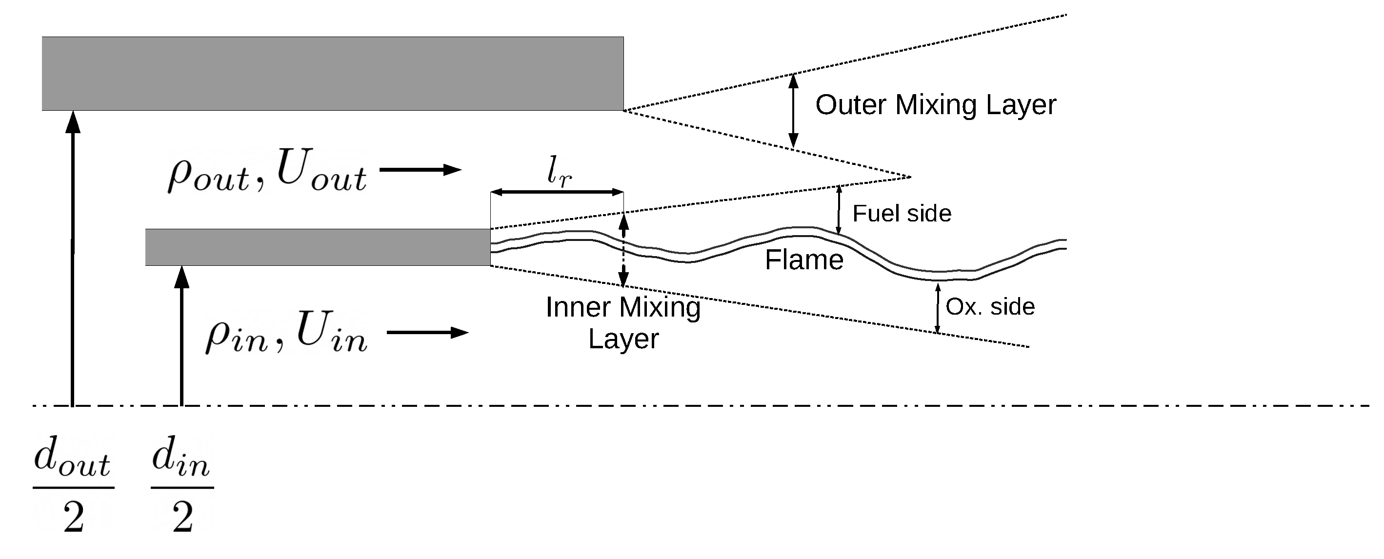
Shear-coaxial injectors are a recurrent design choice for liquid rocket engines. Cases such as the Vulcain II engine and SSME (Space Shuttle Main Engine) [36] are well-known examples. In this type of injector, one propellant (typically the oxidizer) flows through a central tube, and the other (normally the fuel) through a concentric annulus. As both fluids are injected with different axial speeds, an inner-shear layer is formed once both fluids meet. An additional outer-layer is formed between the annular flow and the external environment of the jet. A schematic of the jet structure is shown in Figure 1, where $\rho$ is the density and U the axial velocity component. For convenience, a flame sheet has been superimposed which helps identify an oxidizer side (when the central flow equates to the oxidizer stream) and a fuel side (when the annular flow equates to the fuel stream).

The good mixing qualities of coaxial injectors for liquid propellants have been attributed to the destabilizing aerodynamic forces which act on the central fluid which trigger the breakup of the liquid jet [36]. However, it must be noted that the mechanisms which influence the mixing of the propellants are dependent on the propellant phases and their relative velocities. In such cases where both fluids are in super-critical conditions or gaseous, i.e., in a single phase, the turbulent mixing constitutes the driving mechanism.

For all fluids involved, a velocity ratio ($VR$) larger than unity is desired;

$$VR=\frac{U_{out}}{U_{in}},$$

(1)

where $out$ and $in$ subscripts refer to the inner and outer flows in the coaxial injector. In such cases, the near field of the coaxial jet is characterized by the appearance of hydrodynamic instability which grows, forming three-dimensional vortices, convected downstream by the mean flow. A direct consequence of this instability is thus the formation of interface corrugations which increase the contact area between both streams [37]. This plays a primary role in the overall mixing and entrainment, and consequently heat-release due to increased wrinkling of the resulting diffusion flame. Furthermore, in these highly turbulent flows, the influence of molecular transport is only limited then to the smallest scales of motion and plays no direct role in the mixing rate [38].

Several attempts have been made to enhance the performance of shear-coaxial injectors, either via inducing a swirling motion on the annular flow to induce the development of a transverse instability, or by recessing the central oxidizer post. In the latter case, a pre-reaction and mixing region inside the injection channel is used. Several studies have observed that by recessing the oxidizer post, the two-stream mixing is enhanced, hence leading to faster flame expansion, shortened flame-length, and greater combustion efficiency. Silvestri et al. [39] carried out experiments on a single-element, shear-coaxial, $\mathrm{GOx}/{\mathrm{CH}}_4$ rocket combustor with optical access at varying mixture ratios ($O/F$) and recess lengths ($l_r$). ${\mathrm{OH}}^{*}$ emission images showed for recessed configurations a conical flame shape in the near injection zone, linked to faster expansion, and a displacement upstream of the flame emission zone. In all cases, a larger recess was linked to greater injector pressure loss, in both fuel and oxidizer streams. Additionally, analysis of the wall heat flux and combustion efficiency showed an increase in both for recessed injectors.

Lux and Haidn [40] performed experiments on a $\mathrm{LOx}/{\mathrm{CH}}_4$ single-element combustor for different values of LOx post’s recess length at sub-, near-, and supercritical conditions. ${\mathrm{OH}}^{*}$ emission images show, similarly to [39], when increasing recess, that the emission intensity starts at a higher level shortly behind the methane injection nut, meaning a higher axial gradient of the flame envelope. In all operating conditions, dependency of jet diameter on the momentum flux ratio (J) was reported:

$$J=\frac{{\left(\rho U^2\right)}_{out}}{{\left(\rho U^2\right)}_{in}}.$$

(2)

Combustion roughness was observed to decrease; however, strong hydrodynamic instabilities were observed on the surface of the LOx jet.

Kendrick et al. [41] performed similar studies on a single-element, shear-coaxial $\mathrm{LOx}/{\mathrm{H}}_2$ rocket combustor. Overall, similar flame behavior was observed. The enhanced mixing and earlier break-up of the central LOx core was attributed to the development of the flame inside the injector in the recessed configuration, which caused a premature expansion of the gases and consequently accelerated the gaseous ${\mathrm{H}}_2$ flow, increasing the effective momentum–flux ratio. Finally, Juniper and Candel [42] studied the stability of two-dimensional wake-like ducted compound flow. They demonstrated that recessing the central tube of a coaxial injector leads to self-sustained wake-like instabilities of the central stream.

3. Materials and Methods

In this work, data-driven surrogate models were derived from a dataset of ∼100 large eddy simulations (LES) carried out with the code AVBP [43]. The models target a given scalar QoI—the flame-length or characteristic velocity ($c^{*}$), and 2D field time-averaged maps, such as the average temperature (T), oxygen mass fraction ($Y_{O_2}$), and mixture-fraction field maps. In addition, thanks to the transient nature of LES, root-mean-square (RMS) 2D maps of the velocity-u ($u_{RMS}$) component were also predicted.

The simulated case corresponds to a single-element, $\mathrm{GOx}/{\mathrm{CH}}_4$ shear-coaxial injector and a partial section of the combustion chamber. Three design parameters were considered during the design of experiments (DOE): two geometrical, namely, the recess length ($l_r$) and the chamber radius ($d_c$), and one operating-point parameter, the mixture ratio ($O/F$).

3.1. Coaxial Injector LES Configuration

The compressible and reactive Navier–Stokes (NS) CFD solver AVBP was used. The equations solved were the Favre-averaged three-dimensional NS filtered equations [44]. The base configuration of the injector hereby described was inspired by the experimentally tested single-element combustion chamber at the Tehcnische Universtität München (TUM). For more details on this, the reader may refer to [45,46,47]. Specifically, the geometry was simplified by considering a circular cross-section chamber having in the base configuration, the same cross-section area as the reference experimental case. A representative 2D longitudinal cut is depicted in Figure 2a, where the fuel and oxidizer injection and outlets are identified. A 30° wedge cut is considered, with lateral periodic boundary conditions, as shown in Figure 2b. Only the first third of the chamber length is considered. The combustion chamber and injection channel lengths were set thus to $l_c=96.67$ mm and $l_{inj}=40$ mm, respectively. To prevent numerical issues at the axis location, the wedge tip was removed at a height $g_{\alpha }=0.25$ mm, and the resulting patch redefined as a slip surface. The tip height is $d_t=0.5$ mm, the oxidizer–injector’s radius is $d_{ox}=2.0$ mm, and the fuel injector’s height is $d_f=0.5$ mm.

Homogeneous mass fluxes of gaseous oxygen (${\dot{m}}_{ox}$) and methane (${\dot{m}}_f$) at 278 and 269 K, respectively, are imposed at the inlets. Total mass flow is not a parameter that is varied in the dataset, and it is fixed to a reference (the chosen value corresponds to the tests in [47]) value of $0.062\mathrm{kg}·{\mathrm{s}}^{-1}$. A constant pressure of $P_{out}=20$ bar was set at the outlet. All inlets and outlet have Navier–Stokes characteristic boundary conditions (NSCBC) [48] imposed to handle the exiting acoustics waves from the modeled domain. In the specific case of inlets, a non-reflective inlet (NRI) [49] was chosen. No turbulence injection was considered as a first approach.

Injection channel walls and the injection plane, sketched with dark lines in Figure 2a, are treated as adiabatic slip walls to further decrease the computational complexity. The chamber wall, shown as “WALL TOP” in Figure 2a (gray line) and Figure 2b, is treated as a conducting, $1$ mm thick copper surface (the thermal conductivity of copper is taken as ${\kappa }_{\mathrm{Cu}}=401.0\frac{\mathrm{W}}{{\mathrm{m}}^2\mathrm{K}}$). A homogeneous and constant external temperature $T_s=350$ K was applied on the dry-surface side. A thermally coupled wall-law [50] was chosen as wall model to reduce the cost per sample. The pertinence of the choice of wall-model and its accuracy is out of the scope of this project and will be addressed in future studies.

The numerical schemes used are the Lax-Wendroff scheme (LW) [51] for the convective terms and a 4th-order finite-element scheme for the diffusive terms ($\mathrm{FE}4\Delta$). The limit CFL number was set to $0.7$, whereas to prevent spurious oscillations originating from the numerical schemes, a $2\mathrm{nd}$-order artificial viscosity (AV) between 0.1 and 0.15 and $4\mathrm{th}$-order AV of 0.01 were applied locally in zones of high gradients. A sigma ($\sigma$) model [52] is used for closure of the subgrid-scale stresses.

The reacting oxy-methane mixture is treated as a perfect gas with a global chemistry scheme optimized to capture the proper heat-release rate to a pressure similar to the operating one ($P_c\approx 18.5$ bar). The scheme is composed of six species, namely, ${\mathrm{O}}_2$, ${\mathrm{CH}}_4$, CO, ${\mathrm{H}}_2\mathrm{O}$, ${\mathrm{CO}}_2$, and ${\mathrm{H}}_2$; and four chemical reactions:

$$\begin{array}{c}{\mathrm{C}\mathrm{H}}_4+\frac{1}{2}{\mathrm{O}}_2\to \mathrm{C}\mathrm{O}+2{\mathrm{H}}_2\hfill \\ {\mathrm{C}\mathrm{H}}_4+{\mathrm{H}}_2\mathrm{O}\to \mathrm{C}\mathrm{O}+3{\mathrm{H}}_2\hfill \\ {\mathrm{H}}_2+\frac{1}{2}{\mathrm{O}}_2\rightleftharpoons {\mathrm{H}}_2\mathrm{O}\hfill \\ \mathrm{C}\mathrm{O}+{\mathrm{H}}_2\mathrm{O}\rightleftharpoons {\mathrm{C}\mathrm{O}}_2+{\mathrm{H}}_2\hfill \end{array}$$

(3)

An infinitely fast chemistry approximation is not considered, as it is known that for oxy-methane combustion in rocket-engine conditions, chemical timescales approximate that of the turbulent flow at high strain rates [53]. Furthermore, it may also occur that the widely used flamelet approximations are not valid, as the Damköhler number $Da={\tau }_t/{\tau }_c$ is not sufficiently high to decouple the turbulent mixing from chemistry, and instead unsteady effects may appear. The turbulence–combustion interaction (TCI) model is based on turbulent diffusion, which drives the turbulent chemical rates in diffusion flames. For greater insights on this matter, the reader may refer to [47]. To prevent issues associated with stiff chemistry at the expected high strain rates, similar exponential chemistry integration to that of [53] was implemented. In all cases, a fully tetrahedral mesh was used with a resolution at the flame anchoring of at least five points in the tip height. More detail about the mesh sizes obtained in the dataset is shown in Section 3.3. Finally, all cases were run for $2$ ms, which corresponds to approximately four convective times of the flow in the reference case. An example of a longitudinal cut of the instantaneous temperature field is shown in Figure 2c.

3.2. Design of Experiments

The LES configuration of a shear-coaxial injector detailed in Section 3.1 served as the departing point for the data-generation stage. The recess length ($l_r$), combustion-chamber radius ($d_c$), and mixture ratio ($O/F$) were selected as parameters for the design space exploration. As illustrated in the literature and detailed in Section 2, we identified the recess length as a parameter of interest due to its reported strong influence on the flame expansion. To compliment this parameter, the chamber-radius was included to further explore the effects on early flame-expansion. The mixture ratio was selected as a proxy variable to J, given $J\propto {(O/F)}^{-1}$. To define the design-subspace $\mathbb{D}\subset {\mathbb{R}}^3$, different criteria were considered based on each variable.

The recess length was established as $l_r\in [0,15]$ mm. The limit value of $15$ mm corresponds to the extreme value used by Silvestri et al. [39] in their $\mathrm{GOx}/{\mathrm{CH}}_4$ experiments of a recessed single-element shear-coaxial injector. The combustion chamber radius was fixed to $d_c\in [6.7,13.41]$ mm, to keep a confinement ratio $c=A_c/A_{out}$ in the range $[5,20]$, where $A_c$ is the chamber’s cross-section area and $A_{out}$ the injector’s outlet area. Indeed, $c=5.09$ corresponds to the confinement ratio of the reference TUM test-bench, for which was observed strong jet confinement. On the other hand, c greater than 20 is expected to have a less significant impact on the flame behavior. For reference, Schumaker and Driscoll [54] carried out experimental studies on the mixing dynamics of non-reacting coaxial jets with large velocity ratios. They reported that confinement of the jet for the confinement ratios they explored $c=A_c/A_{out}\in [34,74]$ caused less than $3\%$ change in the measured data of stoichiometric mixing lengths.

Finally, the mixture ratio limits were derived from two constraints: First, a minimum velocity ratio $VR\ge V{R}_{inf}=1$, which is linked to a desired flow regime in flush mounted injectors configurations and is typical for rocket-engines. In such regime, a faster annular stream destabilizes the central flow, as explained in [37]. Second, a maximum momentum flux ratio was fixed ($J_{sup}$). Combining the definitions of $VR$ and J, it yields:

$$\left(\frac{A_{ox}}{A_f}\right)\frac{1}{\sqrt{{\rho }_r{J}_{sup}}}\le O/F\le \frac{1}{V{R}_{inf}{\rho }_r}\left(\frac{A_{ox}}{A_f}\right),$$

(4)

where $A_{ox}/A_f$ is the oxidizer to fuel wet-area ratio and ${\rho }_r={\rho }_f/{\rho }_{ox}$ the fuel-to-oxidizer density ratio. For the current value of the area ratio, one obtains, $O/F\le 2.94$ which locates the mixture in a rich regime. To prevent us from simulating very rich mixtures, as these would depart significantly from nominal operating conditions in LREs, the $J_{sup}$ was limited to 5.0. Hence, $O/F\in [2.6,2.94]$. Note that in real-life applications, J may reach values of up to 20.0 [55]. The design of experiments parameters are summarized in

Table 1. Parameter range, reference values, and sampling mode for the three parameters of the design of experiments.

Parameter	Symbol	Range	Reference	Sampling Mode
Recess-length	$l_r$	0–15 mm	0 mm	Linear
Chamber radius	$d_c$	6.7–13.41 mm	6.77 mm	Linear
Mixture-fraction	$O/F$	2.6–2.94	2.62	Linear

.

Having defined the design space, two Latin-hypercube sampling (LHS) samples [56] using the enhanced stochastic evolutionary algorithm (ESE) [57] were obtained via the Surrogate Modelling Toolbox (SMT) [4]. The first one (DS1) consisted of 100 samples, which was intended to cover the training and validation samples once we evaluated their corresponding design points through AVBP, and the second (DS2) of 20 samples, which is to serve as a test dataset for the future data-driven surrogate models.

3.3. Overview of the Coaxial Injectors LES Database

The joint plots for the shear-coaxial injectors LES database are shown in Figure 3. Each point has been labeled in accordance to the dataset it belongs to or “Crash”, which indicates the associated LES simulation did not achieve the target $2$ ms of run-time. Figure 3a shows crashes are evenly distributed in the $l_r-O/F$ plane. However, Figure 3b,c show an accumulation of failed simulations towards higher values of $d_c$. The $d_c$ colored histogram confirms a greater tendency to crash for higher levels of $d_c$. Note that a lower density of samples is thus available in this region of the design-space.

The analysis of the crashed samples indicated that failure location was almost always in an “OUTLET” node. The visualization of the transient flow prior to crashing in some of the samples with higher $d_c$ showed a vortex exiting the domain and generating a local negative pressure gradient at the outlet. This negative pressure gradient would lead to inflow at the “OUTLET” boundary, thus leading to crashing. It is suspected that for these simulations, the NSCBC relaxation coefficient imposed at the outlet boundary condition significantly conditioned the flow at the outlet.

A total of 96 samples, of the planned 120, were thus available between DS1 and DS2 for the elaboration of surrogate models. The average CPU cost per sample was $1488.86$ CPU hours running on 128 cores using AMD Epyc processors at 2.6 GHz. A scatter plot of the CPU hours consumed vs. the number of tetrahedral cells in the mesh on the complete database is shown in Figure 3d. A correlation can be observed between both quantities, which can be linked to the $d_c$, as it has a predominant influence on the mesh volume, and thus the total number of cells.

4. Results: Training the Surrogate Models

In the following paragraphs, the steps leading to the development of data-driven scalar QoIs surrogate models and 2D field quantities are detailed. The approach taken is similar to the one detailed by Krügener et al. [33]. The database of LES simulations of single-element shear-coaxial injectors presented in Section 3.3 served as foundation for the models hereby presented.

4.1. Global Quantities Models

The scalar quantities of interest we considered are the characteristic velocity of the combustion products at the outlet ($c_{les}^{*}$), the integral wall heat flux ($\dot{Q}$) exiting the domain through the chamber wall, and the flame length ($L_{fl}$). Their definitions are given in (Equations (5)–(7)):

$$c_{les}^{*}=\sqrt{{\left(\frac{{\overline{\gamma }}_{out}+1}{2}\right)}^{\left(\frac{{\overline{\gamma }}_{out}+1}{{\overline{\gamma }}_{out}-1}\right)}\frac{{\overline{R}}_{m,out}{\overline{T}}_{0,out}}{{\overline{\gamma }}_{out}}},$$

(5)

$$\dot{Q}={\int }_{A_{WT}}\overrightarrow{q}·\widehat{n}dS,$$

(6)

$$L_{fl}\equiv \underset{x}{\arg }\frac{1}{A\left(x\right)}{\int }_{A\left(x\right)}HR\left(\mathit{x}\right)dS=hr\left(x\right)=0,$$

(7)

where ${\overline{\gamma }}_{out}$, ${\overline{T}}_{0,out}$, and ${\overline{R}}_{m,out}$ are the mean specific-heat ratio, stagnation temperature, and gas constant of the mixture at the outlet; $\overrightarrow{q}$ and $A_{WT}$ are the wall heat flux and top-wall surface area; and $A\left(x\right)$ and $HR\left(\mathit{x}\right)$ are the chamber domain’s cross-sectional area at axial coordinate x and the heat-release field, respectively. The origin frame locates the coordinate $x=0$ in the injection plane. Note that, following the definition from Equation (7) it may occur that for the simulated chamber length $l_c<L_{fl}$, rendering this definition inapplicable. This was observed in several samples of the dataset. However, $hr\left(x\right)$ for $x>l_c/2$ was seen to be a monotonically decreasing smooth function, and therefore, a flame-length proxy, ${\tilde{L}}_{fl}$, was introduced following the definition of $L_{fl}$ and patching $hr\left(x\right)$ with a linear extrapolation for $x>l_c$.

To enable the dataset at hand to be most representative of LREs conditions and prevent non-converged LES simulations or close-to-crash simulations from contaminating the sample, two additional filters were implemented. First, those simulations with negative pressure losses at the injectors $\Delta P_{fuel},\Delta P_{ox}<0$ were removed, where

$$\begin{array}{c}\Delta P_{fuel}={\overline{P}}_{in,fuel}-{\overline{P}}_c,\\ \Delta P_{ox}={\overline{P}}_{in,ox}-{\overline{P}}_c.\end{array}$$

(8)

with ${\overline{P}}_{in,fuel}$, ${\overline{P}}_{in,ox}$, and ${\overline{P}}_c$ being the mean fuel inlet, oxidizer inlet and chamber pressures, respectively. Second, each k QoI extracted from the dataset was normalized following its respective mean (${\mu }^k$) and standard deviation (${\sigma }^k$). Hence, any record i verifying the following condition:

$$z_i^k=\frac{(y_i^k-{\mu }^k)}{{\sigma }^k}>3.0,$$

(9)

was removed from the dataset to alienate extreme outliers. For clarity, ${\mu }^k=1/N_s{\sum }_{i=1}^{N_s}{y}_i^k$ is the mean and ${\sigma }^k=\sqrt{{\sum }_{i=1}^{N_s}{(y_i^k-{\mu }^k)}^2/N_s}$ is the standard deviation, where $N_s$ represents the dataset’s size. Hence, we were left with 74 for training and validation from DS1, and 16 for testing from DS2. Finally, prior to learning, a normalization step for both inputs and outputs of the networks was conducted such that the resulting mapped spaces were well within the $\mathcal{O}\left(1\right)$ order of magnitude. Thus, if the sought map to be provided by the surrogate model is $F:\mathit{x}\in {\mathbb{D}}_x\mapsto y\in {\mathbb{D}}_y$, with ${\mathbb{D}}_x\subset {\mathbb{R}}^3,{\mathbb{D}}_y\subset \mathbb{R}$ the input and output subspaces, respectively, then the map constructed by the neural network shall be $F^{*}:\mathit{u}\in {\mathbb{D}}_u\mapsto q\in {\mathbb{D}}_q$, such that for all $\mathit{x}={(x_1,x_2,x_3)}^T\in {\mathbb{D}}_x$ exists:

$$\mathit{u}={(u_1,u_2,u_3)}^T\mathrm{with}{\left[\mathit{u}\right]}_i=\frac{(x_i-{\mu }_{x_i})}{{\sigma }_{x_i}}$$

(10)

where ${\mu }_{x_i}$ and ${\sigma }_{x_i}$* are, defined as the mean and standard deviation of each of the DOE axis ($l_r$, $d_c$ and $O/F$), which are calculated on the basis of the DS1 samples. A similar definition is used for q, such that $q=(y-{\mu }_y)/{\sigma }_y$, where ${\mu }_y$ and ${\sigma }_y$ are the mean and standard deviation for the y magnitude also determined by the samples of DS1. Note that training a neural network on a normalized quantity renders the loss function agnostic of the QoI span. This simplifies the a posteriori selection of hyperparameter ranges, such as regularization, that may be added to the loss function. In addition, it simplifies the comparison of the loss functions between the different quantities.

The surrogate models derived for each of these quantities consisted of FCNNs with rectified linear unit (ReLU) activation functions. Due to the small sizes of the datasets involved, only shallow networks were considered in this approach. Different multilayer percpetron (MLP) architectures were tested for each of the outputs involved, which have been summarized in

Table 2. Summary of surveyed MLPs architecture for each of the global quantities presented.

Output	${\mathit{k}}_{\mathit{h}}$	${\mathit{k}}_{\mathit{w}}$	LR 1	Batch 2	Weight Decay	Dropout
$c_{les}^{*}$	[1, 2, 3]	[2, 3, 4, 5, 6, 7, 8]	0.012	10	0.0001	0.01
${\tilde{L}}_{fl}$	[1, 2, 3]	[2, 3, 4, 5, 6, 7, 8]	0.012	10	0.0001	0.01
$\dot{Q}$	[1, 2, 3]	[2, 3, 4, 5, 6, 7, 8]	0.012	10	0.0001	0.01

¹ LR: initial learning rate. ² Batch: batch size used during training.

. In it, $k_h$ constitutes the number of hidden layers. It is worth noticing that a constant hidden-layer width ($k_w$) was chosen for the architecture search. The first (input) layer always consisted of three neurons corresponding to each of the axes of the design space. The last layer (output) was left to a single output. As overfitting counter measures, a weight decay regularization type and dropout were used. However, due to the low number of samples at hand, a hyperparameter search emphasizing network size was performed first. In this work, no other regularization techniques, such as $L1$-regularization, were considered, in spite of its potential as an overfitting counter measure.

A grid search was performed best on all the possible pairs ($k_h$, $k_w$) for the best-performing design. The performance metric hereby considered corresponds to the average 4-fold relative error in the test dataset (${\overline{E}}_{r,test}$). Training was performed for each combination over a maximum of 200 epochs. The loss function considered was a conventional mean squared error (MSE) loss. During learning, an Adam optimizer was utilized, and the entire process was conducted by means of the PyTorch library [58] and wandb platform [59].

The predictive performance of each network over its corresponding magnitude k was assessed via the average relative error over the test dataset ${\overline{E}}_{r,test}^k$:

$${\overline{E}}_{r,test}^k=\frac{1}{N_{s,test}}\sum _{i=1}^{N_{s,test}}\frac{|y_i^k-{\widehat{y}}_i^k|}{|y_i^k|},$$

(11)

where $y_i^k$ and ${\widehat{y}}_i^k$ correspond to the true value and prediction, respectively, and $N_{s,test}=\left|DS2\right|$ is the cardinality of the test dataset (DS2). Moreover, due to the relatively small dataset, 4-fold cross validation was executed for every configuration. Note that for the magnitudes treated, $c_{les}^{*}$, ${\tilde{L}}_{fl}$, and $\dot{Q}$ are not in the vicinity of 0 ($0\notin {\mathbb{D}}_y$), which enabled the use of a relative error. In Section 4.4, another metric is introduced to circumvent this issue. The best-performing architectures for each magnitude are identified in

Table 3. List of the best-performing network for each of the presented quantities; and their corresponding architectures, number of trainable parameters, average relative errors, and equivalent Kriging model performance.

Output	Architecture	Trainable Parameters	${\overline{\mathit{E}}}_{\mathit{r},\mathit{train}}$	${\overline{\mathit{E}}}_{\mathit{r},\mathit{val}}$	${\overline{\mathit{E}}}_{\mathit{r},\mathit{test}}$	${\overline{\mathit{E}}}_{\mathit{KRG},\mathit{test}}$
$c_{les}^{*}$	[3, 7, 7, 1]	92	0.47%	0.85%	0.86%	0.73%
${\tilde{L}}_{fl}$	[3, 2, 1]	11	4.47%	5.46%	3.17%	4.13%
$\dot{Q}$	[3, 2, 1]	11	2.97%	3.43%	2.63%	3.4%

alongside their 4-fold cross validation relative errors. The corresponding performance of another mainstream surrogate modeling technology, i.e., a Gaussian process (also known as Kriging), is also shown for benchmarking purposes. (GP results were obtained via the SMT package [4] implementation of Kriging (KRG in the documentation). A linear model was utilized for the deterministic term in the interpolating Kriging model, whereas a well-known squared exponential (Gaussian) function was chosen as the correlation function. The Kriging hyperparameters’ optimization was handled by means of a Cobyla optimizer.)

The figures of merit shown in Table 3 indicate some dispersion among the different magnitudes studied. The best performance was attained for $c_{les}^{*}$ of ${\overline{E}}_{r,test}=0.86\%$ and the worst for ${\tilde{L}}_{fl}$ of 3.17%. It is important to remark that for each of these magnitudes, an additional hyperparameter optimization for the winning architectures, involving the initial learning-rate, batch size, weight decay, learning rate decay, and dropout was conducted. However, no consistent improvement in results was observed from this process, and thus, the results were not included.

4.2. Global Quantities’ Error Distribution

In Section 3.2, it is mentioned that the original 120 simulations targeted in the DOE for both DS1 and DS2 were not possible due to the sudden “crashes” in some LES simulations. The distribution of the crashes is inhomogeneous; a greater density was observed for $d_c>1\times {10}^{-2}$ m, as shown in Figure 3b,c. Due to the reduced amount of samples in this specific region of the design space, it is a priori unknown if the surrogates ’prediction capabilities was preserved or locally affected, as no information about the samples distribution in the design space was embedded into the surrogates. Figure 4a–c correspond to scatter plots of the relative error for the each of the DS2 samples (test datasets) with respect to their $d_c$ coordinates, computed for $c_{les}^{*}$, ${\widehat{L}}_{fl}$ and $\dot{Q}$. The best-performing MLPs are detailed in Table 3, for the four iterations of the described cross validation.

In spite of having only few samples in DS2 within the $d_c>1\times {10}^{-2}$ m region (only 4), there appears to be no conclusive evidence on the increase in $E_r$ for all the quantities involved. Indeed, in all three predicted quantities, at least one sample had significantly higher error than the average for all four iterations, although no trend can be observed. (Samples in Figure 4 are identified by their unique $d_c$ coordinates. Variations along the abscise correspond to the results given by the different folds.) Nevertheless, note that in Figure 3c, these samples are concentrated in the $l_r\le 1\times {10}^{-2}$ m region, leaving a lack of test samples for $l_r\ge 1\times {10}^{-2}$ m, where coincidentally most of the crashes were observed. The validity of the surrogates in this corner of the design space therefore remains an open subject of study.

4.3. Navigating the Design Space

A straightforward application of the surrogate models pointed out in Table 3 consists of utilizing one to generate charts for navigating the surveyed design space. These provide qualitative insights on the responses of the QoIs to a given design parameter. Figure 5a–f present the evolution of $c_{les}^{*}$, $\dot{Q}$, and ${\tilde{L}}_{fl}$ in terms of the recess length $l_r$ and the chamber radius $d_c$ for specific mixture ratios $O/F$, as predicted by the associated surrogate models.

Similarly to the experimental observations from [39], the DL-based surrogates show an increase in the characteristic velocity $c_{les}^{*}$ at higher levels of recess in moderate to highly confined flames. Both $l_r$ and $d_c$ have a strong influence on this global quantity, as seen from Figure 5a,b. Curiously, an increment in recess impacts negatively $c_{les}^{*}$ for less confined flames. At a value of $O/F=2.77$, Figure 5b shows a larger plateau for $c_{les}^{*}$. This comes as a result of the higher temperature of gases at the outlet when moving closer to global stoichiometry. As for the total wall heat flux $\dot{Q}$, Figure 5c,d show a strong dependence with the recess length, in particular, for confined flames in which a higher $l_r$ significantly increases $\dot{Q}$ even though the wet area reduces due to a decreasing $d_c$. These tendencies recovered are in accordance to what can be observed experimentally.

Finally, the estimated flame length surrogates prediction, as shown in Figure 5e,f, exhibits a similar topology for both $O/F=2.64$ and 2.77; the former has an accentuated response with respect to the latter. Increasing the recess length does have a tendency to provide shorter flames. Likewise, a less confined flame decreases the flame length. Both phenomena may potentially be linked to a faster expansion of the hot gases in the vicinity of the injection plane, albeit with different underlying mechanisms causing the faster expansion. Note that in spite of observing variation in $L_{fl}$ for the design-space explored, it still remains within $\Delta L_{fl}<15\%{\mu }_{L_{fl}}$ for the figures displayed, comparable to the average relative error for this magnitude presented in Table 3 of $\sim 3\%$.

4.4. Field Quantities Models

In addition to the global quantities models, a series of two-dimensional (2D) field quantities surrogate models was developed. Having access to the 2D fields enriches the analysis of design-space exploration stemming from global quantities charts, as it provides a powerful tool for the physical interpretation of the underlying phenomena. The concerned quantities were: the time-averaged temperature field ($\overline{T}$), the time-averaged oxygen mass fraction field (${\overline{Y}}_{O_2}$), the mixture-fraction field ($\overline{\Xi }$), the time-averaged u-velocity field ($\overline{u}$), and the root-mean-squared u-velocity field ($u_{RMS}$). The $u_{RMS}$ field was computed from the LES time-average solution of the velocity field, and its moment by:

$$u_{RMS}=\sqrt{\overline{u^2}-{\overline{u}}^2}.$$

(12)

The data consisted of the same simulations belonging to DS1 and DS2 presented in Section 3.2. The output of the models was a $128\times 256=\mathrm{32,768}$ cells field. The larger number of cells was allotted to the longitudinal (x) axis of the injector. For such reason, on each sample from DS1 and DS2, the concerned three-dimensional LES solution fields were interpolated to a $128\times 256$ grid lying on the $z=0$ plane. To account for the fact that areas in the aforementioned rectangular grid would be outside the wet perimeter of the injector’s domain, another 2D grid, from now on denoted as mask, $\mathit{M}$, was introduced following the definition:

$${\left[{\mathit{M}}^i\right]}_{pq}\in {\mathbb{R}}^{128\times 256}=\{\begin{array}{c}1\mathrm{if}(x_q,y_p)\in {\Omega }_i\hfill \\ 0\mathrm{if}(x_q,y_p)\notin {\Omega }_i.\hfill \end{array}$$

(13)

where i is the samples’ index in the dataset, ${\Omega }_i$ the volume associated with it, and $(x_q,y_p)$ the corresponding geometrical coordinates of the $pq$ grid element in the interpolating grid. Note that ${\mathit{M}}^i$ encodes geometrical information about the injector and hence the location of the relative i sample in the design-space.

The problem of interest is then to construct a map $H^k:\mathit{x}\in {\mathbb{D}}_{\mathit{x}}\mapsto {\mathit{y}}^k\in {\mathbb{D}}_{{\mathit{y}}^k}$ where ${\mathbb{D}}_{\mathit{x}}\subset {\mathbb{R}}^3$, ${\mathbb{D}}_{{\mathit{y}}^k}\subset {\mathbb{R}}^{128\times 256}$, and k is an index introduced for convenience to denote one of the field quantities mentioned. The subspace ${\mathbb{D}}_{\mathit{x}}$ is the input space of the map where $\mathit{x}={(x_1,x_2,x_3)}^T$ nucleates the three design-space parameters $l_r$, $d_c$, and $O/F$. Similarly to what was explained in Section 4.1, a “normalized” map can be defined as $H^{*,k}:\mathit{u}\in {\mathbb{D}}_{\mathit{u}}\mapsto {\mathit{q}}^k\in {\mathbb{D}}_{{\mathit{q}}^k}$. On the one hand, $\mathit{u}$ follows the definition given in Equation (10), whereas on the other hand, ${\mathit{q}}^k$ is given by:

$$\{\begin{array}{c}{\left[{\mathit{q}}^k\right]}_{mn}=\frac{({\left[{\mathit{y}}^k\right]}_{mn}-{\mu }^k)}{{\sigma }^k}\hfill \\ {\mu }^k=\frac{1}{N_s{N}_w}{\displaystyle \sum _{m=1}^{N_y}}{\displaystyle \sum _{n=1}^{N_x}}{\displaystyle \sum _{i=1}^{N_s}}{\left[{\mathit{M}}^i\right]}_{mn}{\left[{\mathit{y}}_i^k\right]}_{mn}\hfill \\ {\sigma }^k={\left(\frac{{\sum }_{i=1}^{N_s}{\sum }_{m=1}^{N_y}{\sum }_{n=1}^{N_x}{\left[{\mathit{M}}^i\right]}_{mn}({\left[{\mathit{y}}_i^k\right]}_{mn}-{\mu }^k)}{N_s{N}_w}\right)}^{1/2}\hfill \end{array}$$

(14)

where $N_w={\sum }_{i=1}^{N_s}{\sum }_{m=1}^{N_y}{\sum }_{n=1}^{N_x}{\left[{\mathit{M}}^i\right]}_{mn}$, $N_x=256$, $N_y=128$ and $N_s=\left|\mathrm{DS}1\right|$. The filters applied over the global dataset described via Equations (8) and (9) were also applied for the field quantities for consistency.

The 2D regression task expressed by $H^{*,k}$ is tackled with a variant of the CNN, known as U-Net [60], including batch normalization that has up-sampling layers, and skip connections. CNNs have been extensively used on two-dimensional data, e.g., for image processing, though more recently for simulation tasks, as exemplified previously in Section 1. The present network architecture, shown in Figure 6, is similar to the one deployed by Krügener et al. [33] for their 2D temperature field model from RANS numerical data of LRE injectors. In this work, U-Nets were chosen as a consequence of the observations from Krüegener et al. [33], whose U-Net reported a slight better accuracy compared to a conventional CNN in the emulation of an LRE injector temperature field. This trend was accentuated when incorporating field gradient information into the training loss function. Note that these findings only pertain to a smooth 2D field, i.e., time-averaged temperature field, albeit it is unknown if they can be extended to more complex field topologies, such as that of $u_{RMS}$, presented in the next sections. Future works will concentrate on benchmarking the U-Net findings to other DL techniques, such as MPLs and GNNs. Finally, in similar fashion to the approach taken in [33], the proposed map $H^{*,k}$ was slightly modified to include the mask as input such that the final sought map is:

$$H^{†,k}:(\mathit{u},\mathit{M})\in {\mathbb{D}}_{\mathit{u}}\times {\mathbb{R}}^{128\times 256}\mapsto {\mathit{q}}^k,$$

(15)

with $\mathit{M}$ encoding information about the geometry, although to a coarse resolution determined by the interpolation grid. The components of $\mathit{u}=(u_1,u_2,$ and $u_3{)}^T$ are handed to the U-Net as homogeneous 2D grids of $128\times 256$ with constant values.

A Bayesian optimization of the U-Net hyperparameters was carried out for each FQ k with the aim of minimizing the 10-fold cross validation prediction error. The 10-fold cross validation was obtained after the splitting of the pairs $({\mathit{x}}_i,{\mathit{y}}_i^k)$ belonging to DS1, into training and validation sets, whereas those belonging to DS2 were reserved for testing. The prediction error was evaluated as the average grid-cell relative error over a set of $N_s$ samples:

$${\overline{E}}_r^k=\frac{1}{N_s{N}_w}\sum _{m=1}^{N_y}\sum _{n=1}^{N_x}\sum _{i=1}^{N_s}{\left[{\mathit{M}}^i\right]}_{mn}\frac{|{[{\mathit{y}}_i^k]}_{mn}-{[{\widehat{\mathit{y}}}_i^k]}_{mn}|}{|{\left[{\mathit{y}}_i^k\right]}_{mn}|},$$

(16)

for those FQs where $|{\left[{\mathit{y}}_i^k\right]}_{mn}|>0$, i.e., $\overline{T}$. For the cases in which this constraint is not feasible, due to the nature of the field being predicted, an average grid-cell normalized error is presented in the form:

$${\overline{E}}_n^k=\frac{1}{N_s{N}_w}\sum _{m=1}^{N_y}\sum _{n=1}^{N_x}\sum _{i=1}^{N_s}{\left[{\mathit{M}}^i\right]}_{mn}\frac{|{[{\mathit{y}}_i^k]}_{mn}-{[{\widehat{\mathit{y}}}_i^k]}_{mn}|}{|{\mu }^k|}$$

(17)

with ${\mu }^k$ following the definition given in Equation (14). In these definitions, ${\widehat{\mathit{y}}}_i^k$ is the k-data-driven model prediction for entry i of the dataset.

All the tested networks were made of 13 hidden layers with a total number of trainable parameters of 486,337. The hyperparameters’ optimization was carried in an a100 GPU by means of PyTorch and the wandb framework. An Adam optimizer was utilized during training in combination with a mixed loss function of the form

$$L={\alpha }_{\mathit{MSE}}\mathit{MSE}+{\alpha }_{\mathit{GDL}}\mathit{GDL}.$$

(18)

The loss L is a linear combination of two terms: first, a conventional MSE loss function, and second, a gradient difference Loss. The latter penalizes the learning process on the basis of the difference between the finite-difference gradients of the ground truth and predicted FQ calculated within the grid. The rigorous definition for GDL, adapted from Equation (24) of [33], is:

$$\begin{array}{c}\hfill \mathrm{GDL}(y^k,{\widehat{y}}^k)=\frac{1}{N_s}\sum _{i=1}^{N_s}\sum _{m=1}^{N_y}\sum _{n=1}^{N_x}{[{\mathit{M}}^i]}_{m,n}\left\{\right||({[{\mathit{y}}_i^k]}_{m,n}-{[{\mathit{y}}_i^k]}_{m-1,n})-({[{\widehat{\mathit{y}}}_i^k]}_{m,n}-{[{\widehat{\mathit{y}}}_i^k]}_{m-1,n}){\left|\right|}^2\\ \hfill +\left|\right|({[{\mathit{y}}_i^k]}_{m,n}-{[{\mathit{y}}_i^k]}_{m,n-1})-({[{\widehat{\mathit{y}}}_i^k]}_{m,n}-{[{\widehat{\mathit{y}}}_i^k]}_{m,n-1}){\left|\right|}^2\}.\end{array}$$

(19)

Note that following Equation (18), both weights ${\alpha }_{MSE}$ and ${\alpha }_{GDL}$ tune the relative importance of each term’s contribution to the loss, although their direct comparison is misleading, as MSE and GDL may well occupy different orders of magnitude.

The summary of the hyperparameters’ Bayesian optimization, the intervals used for the search, and corresponding quantization for each of the magnitudes involved are given in

Table 4. List of hyperparameters we varied, their preset intervals, and quantization for each of the field quantities models provided. The map style has also been included to identify category of map elaborated by the resulting surrogate model.

Description		$\overline{\mathit{T}}$	${\overline{\mathit{Y}}}_{{\mathit{O}}_2}$	$\overline{\mathit{\Xi }}$	$\overline{\mathit{u}}$	${\mathit{u}}_{\mathbf{RMS}}$
Map style		$H^{†,k}$	$H^{†,k}$	$H^{†,k}$	$H^{†,k}$	$H^{†,k}$
Batch size	Values	[4, 8]	[4, 8]	[4, 8]	[4, 8]	[4, 8]
Initial LR	Range	0.001–0.01	0.0001–0.001	0.0001–0.001	0.0001–0.01	0.001–0.01
Dropout	Range	0–0.02	0–0.02	0–0.02	0–0.02	0–0.02
	Quantization	0.005	0.005	0.005	0.005	0.005
LR Decay 1	Range	0.81–0.99	0.85–0.99	0.85–0.99	0.85–0.99	0.81–0.99
	Quantization	0.02	0.01	0.01	0.01	0.02
Weight Decay	Range	0–0.1	0–0.1	0–0.1	0–0.1	0–0.1
	Quantization	0.02	0.02	0.02	0.02	0.02
${\alpha }_{GDL}$	Range	50–80	0–20	0–100	0–100	50–100
	Quantization	10	2	10	10	10

¹ LR Decay: learning rate decay used by the Adam optimizer.

.

To complement the values presented in Table 4, it is worth saying that all the training sessions were conducted over a maximum of 500 epochs with a constant ${\alpha }_{MSE}=1$. Certain parameters shown in Table 4 had different ranges and quantization for different FQs. This was specially the case for ${\alpha }_{GDL}$. As noted previously, the split of the mixed loss function L between MSE and GDL was field-dependent, and therefore, the values of ${\alpha }_{GDL}$ were restricted in certain ranges to prevent saturation due to one loss component. These ranges were obtained through trial and error experiments.

The best-performing configurations obtained in terms of test dataset average relative error (or averaged normalized error) for each of the quantities, calculated from 10-fold cross validation, are displayed in

Table 5. Best-performing networks resulting from the Bayesian hyperparameters’ optimization. The parameters values and the networks performances over the test dataset (DS2) are explained.

Parameter	$\overline{\mathit{T}}$	${\overline{\mathit{Y}}}_{{\mathit{O}}_2}$	$\overline{\mathit{\Xi }}$	$\overline{\mathit{u}}$	${\mathit{u}}_{\mathit{RMS}}$
Batch size	4	4	4	4	8
Initial LR	0.0047	0.00096	0.00097	0.0015	0.00736
Dropout	0.01	0.015	0.01	0.015	0.005
LR Decay	0.98	0.96	0.97	0.97	0.96
Final Epochs 1	499	338	453	467	388
Weight Decay	0	0	0	0	0
${\alpha }_{GDL}$	70	10	30	80	90
% GDL Loss 2	87.5%	57.33%	79.67%	91.84%	93%
Performances
${\overline{E}}_{r,test}$	3.39%	-	-	-	-
${\overline{E}}_{n,test}$	2.86%	4.82%	3.84%	5.3%	9.22%

¹ Even though the maximum number of epochs was 500, the training process may have been stopped before, as convergence was reached. The convergence criteria used during training enforced a loss variation <10⁻⁹. ² % Train GDL Loss corresponds to the relative contribution of the a_GDLGDL term in Equation (18) to the total training loss L.

.

The results shown in Table 5 indicate acceptable global performances in terms of ${\overline{E}}_r$ and ${\overline{E}}_n$, in view of the datasets considered. The batch size in most cases was four, the exception being the $u_{RMS}$ network. The initial learning rate and learning rate decay were seen to be of great relevance in most of the hyperparameter searches conducted. The $\overline{Y_{O_2}}$ and $\overline{\Xi }$ magnitudes showed difficulty in learning for initially large learning rates, which were solved by decreasing them by an order of magnitude during the search. This is evidenced in the considerably lower learning rates for these fields exposed by Table 5. Furthermore, it is shown that the hyperparameters search converged in most cases to null weight decays and moderate to large dropout values. This points towards the fact that we were not experiencing a weight’s explosion, and the enabling mechanism to reduce overfitting was via dropout. Finally, even though the global metrics over the test dataset indicate reasonable accuracies of the 2D surrogates, visual inspection of the fields is necessary to determine the capacity of the U-Net for capturing the relevant structures and regions that make up the injector flow field. This is sine qua non to the interpretability requirement. In Section 5, three points from the design-space not included in the original datasets DS1 and DS2 are surveyed and presented with this aim.

4.5. Field Quantities’ Error Distribution

In similar fashion to what was discussed in Section 4.2, the question of the validity of the predictions from the best performing networks in the $d_c>1\times {10}^{-2}$ m region, where many crashes were evidenced in Section 3.2, is posed. Figure 7a–e are scatter plots of the corresponding error metric versus the $d_c$ coordinate for each sample of DS2 and fold of the 10-fold cross validation, for $\overline{T}$, ${\overline{Y}}_{O_2}$, $\overline{\Xi }$, $\overline{u}$, and $u_{RMS}$, respectively.

Figure 7a ($\overline{T}$) and Figure 7c ($\overline{\Xi }$) show no clear tendency that error increases for this specific region. Instead, it remains comparable to the rest of the samples, hinting that average variations in these fields on this region of the design space are not significant. Surprisingly, for both the ${\overline{Y}}_{O_2}$ and $\overline{u}$ fields the trend indicates that error diminishes with increasing $d_c$. Note that the field response is not homogeneous across the design space, and the U-Net may preserve accuracy over this region in spite of the low sample density during training. The $u_{RMS}$ does not show a clear trend; samples errors alternate around the mean with increasing $d_c$. This may be related to the dependency of the $u_{RMS}$ with other coordinates, such as the $l_r$. The value of error for high-$d_c$ samples may be misleading, as again, no samples in the DS2 dataset are in the $l_r>1\times {10}^{-2}$ m − $d_c>1\times {10}^{-2}$ m corner, as $u_{RMS}$ is highly dependent on $l_r$, which will be shown in the following sections.

5. Results: Surrogate Models’ Analysis and Use to Study the Impact of Recess

To gain further insights on the influence of recess in the development of the flame, three additional LES simulations were performed. The three design points were chosen for a moderately confined flame and $O/F=2.77$, with a varying recess to sample the ${\tilde{L}}_{fl}$ decay observed in Figure 5f when increasing this parameter. Their corresponding values in the design space are listed in

Table 6. Design points inspected during the recessed injector analysis. The values of the LES and MLPs’ prediction global quantities presented in Figure 5b,d,f are provided for completeness.

DP 1	$\mathit{O}/\mathit{F}$	${\mathit{l}}_{\mathit{r}}$ [mm]	${\mathit{d}}_{\mathit{c}}$ [mm]	${\mathit{c}}_{\mathbf{les}}^{*}$ [m/s]		${\widehat{\mathit{L}}}_{\mathbf{fl}}$ [mm]		$\dot{\mathit{Q}}$ [W]
				LES	FCNN	LES	FCNN	LES	FCNN
DP-A	2.77	0	7.5	1461.2	1475.7	117.6	121.8	2029.2	2350.7
DP-B	2.77	7.5	7.5	1516.6	1511.3	116.4	121.8	2621.2	2614.4
DP-C	2.77	14.0	7.5	1538.5	1519.9	112.7	114.9	2887.3	2886.5

¹ DP: Design Point denomination.

. Their calculated global quantities, as extracted from the LES, and those predicted by the surrogate models presented in Table 3, have been included in Figure 5b,d,f for reference. The setup utilized is identical to the one detailed in Section 3.1 and used in DS1 and DS2. Figure 8a–c show the average temperature field estimation from its corresponding U-Net. Additionally, the ${\overline{Y}}_{O_2}\in [0.1,0.8]$ and $\overline{\Xi }=Z_{st}=0.2$ iso-lines, as provided by the models described in Section 4.4, are shown on top.

5.1. Analysis of Average Fields

Figure 8a–c show evidence that the surrogate models are capable of generating realistic predictions of the concerned fields. For reference, the corresponding LES simulation fields, interpolated in the $256\times 128$ grid, are shown in Figure 9a–c. The homogeneous low-temperature in the injection channel is well-preserved, showing only minor fluctuations. Furthermore, the cold methane stream downstream of the injection plane is well resolved in all the evaluated design points.

As for the impact of recessing the oxidizer post, the surrogate model captures its effect well. This is primarily observed in the overall higher temperature of the recirculation zone, located just downstream of the injection plane ($0\mathrm{m}\le x\le 0.02\mathrm{m}$), which occurs when increasing $l_r$. The higher temperatures in the recirculation zone can be attributed to a faster flame expansion, a phenomenon observed experimentally via ${\mathrm{OH}}^{*}$ imaging by Silvestri et al. [39] and Lux et al. [40]. The presence of hotter gases in the recirculation region, and consequently in the top wall, explains partially the greater total wall heat-flux observed in Figure 5d when $l_r$ is incremented. More importantly, the U-Net was able to resolve the flame anchoring point for the studied points. This was not only verified from the topology of $\overline{T}$, but also from the relative locations of the ${\overline{Y}}_{O_2}$ and $\overline{\Xi }$ iso-lines. It is remarkable that in spite of having trained dedicated networks to a given field, with complete ignorance of each other, the obtained outcomes appear intertwined and enable a holistic interpretation. This is explained by the fact that the U-Net accurately represents the coherent underlying LES data.

The analysis of the iso-lines also provides insight on the effect of recess. Fist, note that ${\overline{Y}}_{O_2}$ does not intersect at the axis, but rather approaches it asymptotically due to the symmetry boundary condition imposed where the axis line has been removed. This was done to prevent numerical issues from arising, in spite of artificially affecting the local flow profile in its vicinity, the turbulence development, and hence, mixing. This asymptotic approach was also observed in the raw LES data, proving that it is not a spurious effect of the CNN. The iso-lines all seem to originate from the injector lip. However, in all the figures, a small iso-line portion of the ${\overline{Y}}_{O_2}$ field is close to the inlet of the methane injection channel. This is an inaccurate prediction of the network, as this section is composed of pure methane. The reason for this is yet unknown, although it is suspected that large homogeneous regions in the grid are troublesome for the current U-Net architecture, and thus numerical data are being leaked to this area. In addition, non-physical fluctuations are seen in these lines at the end of the chamber, in particular, near the outlet.

Visual inspection of Figure 8a,c shows displacement of the iso-lines upstream when $l_r$ increases. Both ${\overline{Y}}_{O_2}=0.1$ and ${\overline{Y}}_{O_2}=0.8$, and the $Z_{st}$ curve display greater concavity as the oxidizer post is recessed, hinting to faster oxygen consumption, and eventually a shorter flame.

On the one hand, the average temperature predictive error fields for DP-A and DP-C are shown in Figure 10a,b, respectively. The ${\overline{Y}}_{O_2}\in [0.1,0.8]$ and $\overline{\Xi }=Z_{st}=0.2$ iso-lines, both from the U-Net estimate and ground-truth LES, have been included. The former is designated by the dashed pattern and the latter by the dotted one. Note that the color scale has been saturated to (−250 K, 250 K), which corresponds to $\sim 7.5\%$ of the mixture’s adiabatic flame temperature. The error fields provide great insight on the surrogate performance. The most problematic area is that of the injector’s near-field, in particular, where the flame is located. It is suspected that, with the flame being a region of high temperature gradients, and consequently a thin structure, even small errors in its spatial placement and thickness by the U-Net constitute the causes of the large errors. These errors appear of opposite sign, and zero-in on the vicinity of the $Z_{st}$ lines. In the remaining area of the combustion chamber, the error decreases, although not to 0. The smallest error was obtained in the injection zone, where the temperature was the most homogeneous. Nonetheless, fictitious oscillations are clearly shown, which were also mentioned in previous paragraphs.

The iso-lines predicted by the CNNs show good agreement with those extracted from the LES average solution. The greatest mismatch can be observed in Figure 10a for the $Z_{st}$ line, where the U-Net shows greater concavity and hence a lower y coordinate towards the second half of the chamber.

5.2. $u_{RMS}$ Field Analysis

The advantage of doing LES over RANS lies on the fact that it provides information about the dynamic of the flow. This opens another avenue by which to analyze and interpret the effect of a parameter, such as $l_r$, on the injector flow field and combustion. To garner this capability from the LES database, in Section 4.4 a model for the $u_{RMS}$ quantity was introduced. This was constructed with a map of the type: $H^{†,k}:(\mathit{u},\mathit{M})\mapsto {\mathit{q}}^k$. The estimated $u_{RMS}$ fields given by this U-Net for the design points listed in Table 6 are given in Figure 11a–c, respectively. The $\overline{\Xi }=Z_{st}=0.2$ predicted isoline has been included to denote the approximate average location of the flame.

The $u_{RMS}$ surrogate model, for all the cases involved, shows a complex topology with concentrated intensity in the near field of the injectors, but then reduced for $x\ge 0.04$ m. The U-Net was able to reproduce the locations of the inner and outer shear-layers of the injectors. Note that in the base configuration of the injectors, detailed in Section 3.1, no turbulence injection is included in the GOx and ${\mathrm{CH}}_4$ channels. Hence, the starting point of the velocity fluctuations comes downstream of the injection lip, as a consequence of the presence of the flame and the development of a hydrodynamic instability, which develops at the inner-shear layer. This phenomenon, observed in the LES simulations, was recovered by the surrogate model.

Figure 11a–c elucidate the effects of recessing the oxidizer post over the velocity-u fluctuations. For reference, the corresponding LES simulation $u_{RMS}$ values, interpolated in the $256\times 128$ grid, are shown in Figure 12a–c. In spite of the low grid resolution used ($256\times 128$), it is clearly visible that the $u_{RMS}$ exhibits a strong response in the near field of the coaxial jet when augmenting $l_r$. When zooming in on the region $0\mathrm{mm}\le x\le 0.02$ m in Figure 11a, we can distinguish two structures on opposite sides of the stoichiometric line. A zoom is conveniently provided in Figure 13a, which shows an upper lobe growing from the upper shear layer until $x\sim 0.01$ m, and a lower lobe which spreads along the growth path of the hydrodynamic instability of the oxidizer side of the inner shear-layer. Due to their low intensity and the presence of a dissipative flame, these two structures do not commingle and have a limited impact on the flame considering mixing and wrinkling. When inspecting the plot of the error on the predictions of $u_{RMS}$ prediction on DP-A shown in Figure 14a, it is clear that larger errors are attained in the near field. In particular, the upper-lobe region shows a considerable underprediction, and the surrogate model does not recover the fluctuations of the fuel side of the inner layer, which should coalesce with those of the outer shear-layer, as noted by the authors in [61].

Figure 11b,c shows recessed cases and both a development of an inner shear-layer within the recess zone and a stronger start of the outer-shear layer. This is better observed in the close-up of the DP-C near-field given in Figure 13b. Note that, in recessed injectors, the ducted premature combustion of the propellants accelerates the flow, particularly the cold methane. This is better seen through the estimations of the $\overline{u}$ model, in Figure 15a,b, of DP-A and DP-C, respectively. The axial velocity increment in the vicinity of the injection plane for a vertical coordinate $y\sim 2.5$ mm is evident in the latter, which corresponds to the region where cold methane is injected. Due to the flow acceleration, velocity gradients expected in the outer-shear layer are considerably higher, triggering the generation of stronger vortices, and thus, velocity-u fluctuations. These vortices are convected downstream. Similarly to the flush-mounted configuration (DP-A), the inner-shear layer develops a hydrodynamic instability which slowly grows along the recess zone. Nonetheless, velocity-u fluctuations remain low, which may be explained due to the presence of the flame. Vortices on the fuel rich side of the inner-shear layer eventually meet those from the outer-shear layer close to the inflection point of the stoichiometric line, leading to a strong fluctuation volume. At this point, the commingled turbulent structures have a direct influence on the flame. Strong wrinkling, stretch, and displacement of the flame surface can be observed, which may suggest more intense combustion. In similar fashion, experiments carried out by Lux et al. [40] in a supercritical LOx/methane rocket combustor reported larger scattering of the flame emission zone when recessing the oxidizer post.

6. Conclusions

Competition in the launch services sector is projected to increase considerably in the coming years. There is a strong drive from different stakeholders to decrease development, manufacturing, and operation costs. High-fidelity simulations of rocket engine combustion have become a relevant tool in everyday engineering and are one of the key enabling technologies to continue driving costs down. Regardless, to this date and with contemporary computing architectures, there still are several challenges associated with their computational costs. Data-driven surrogate models provide a temporal alternative to circumvent these issues.

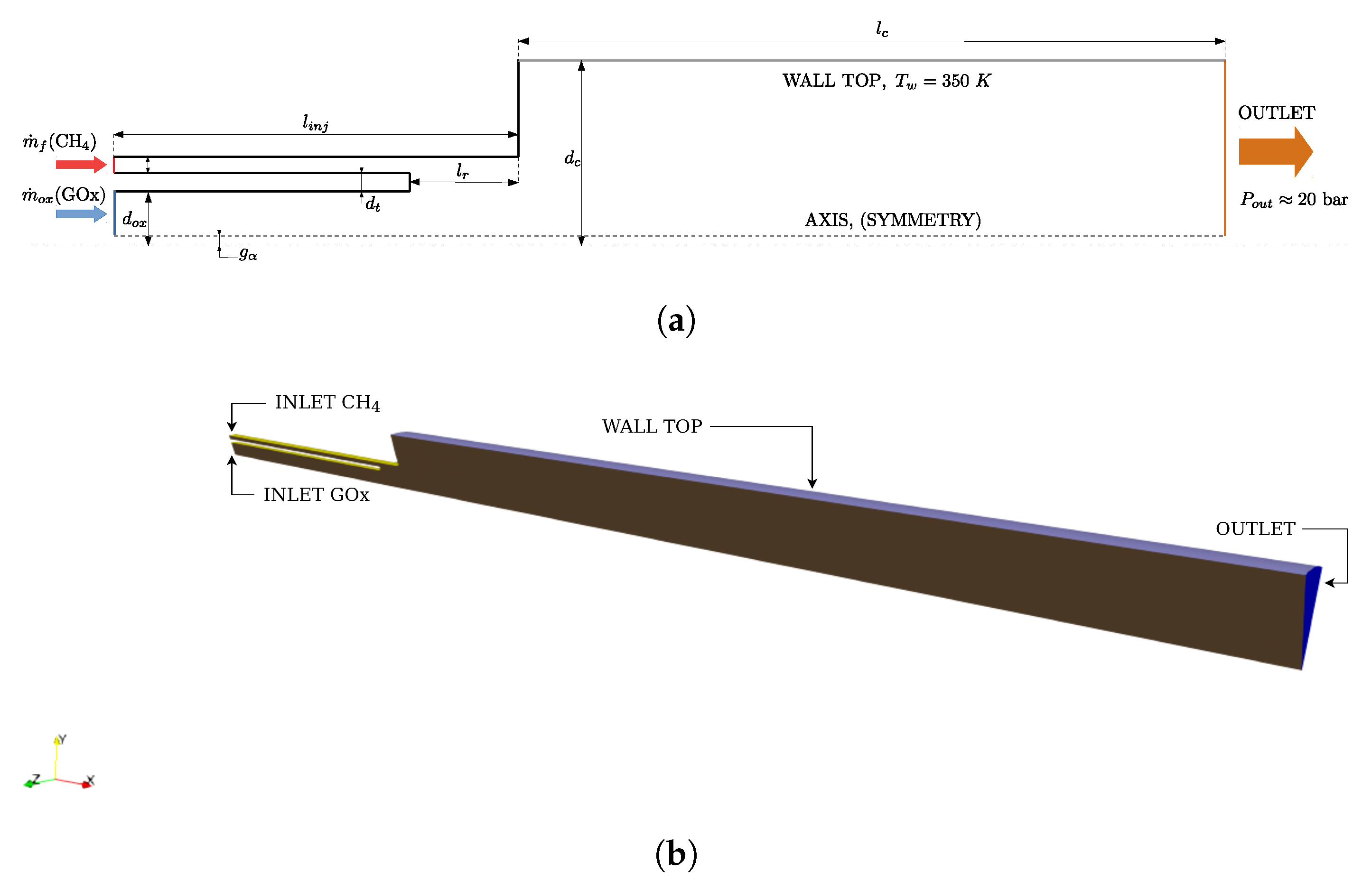
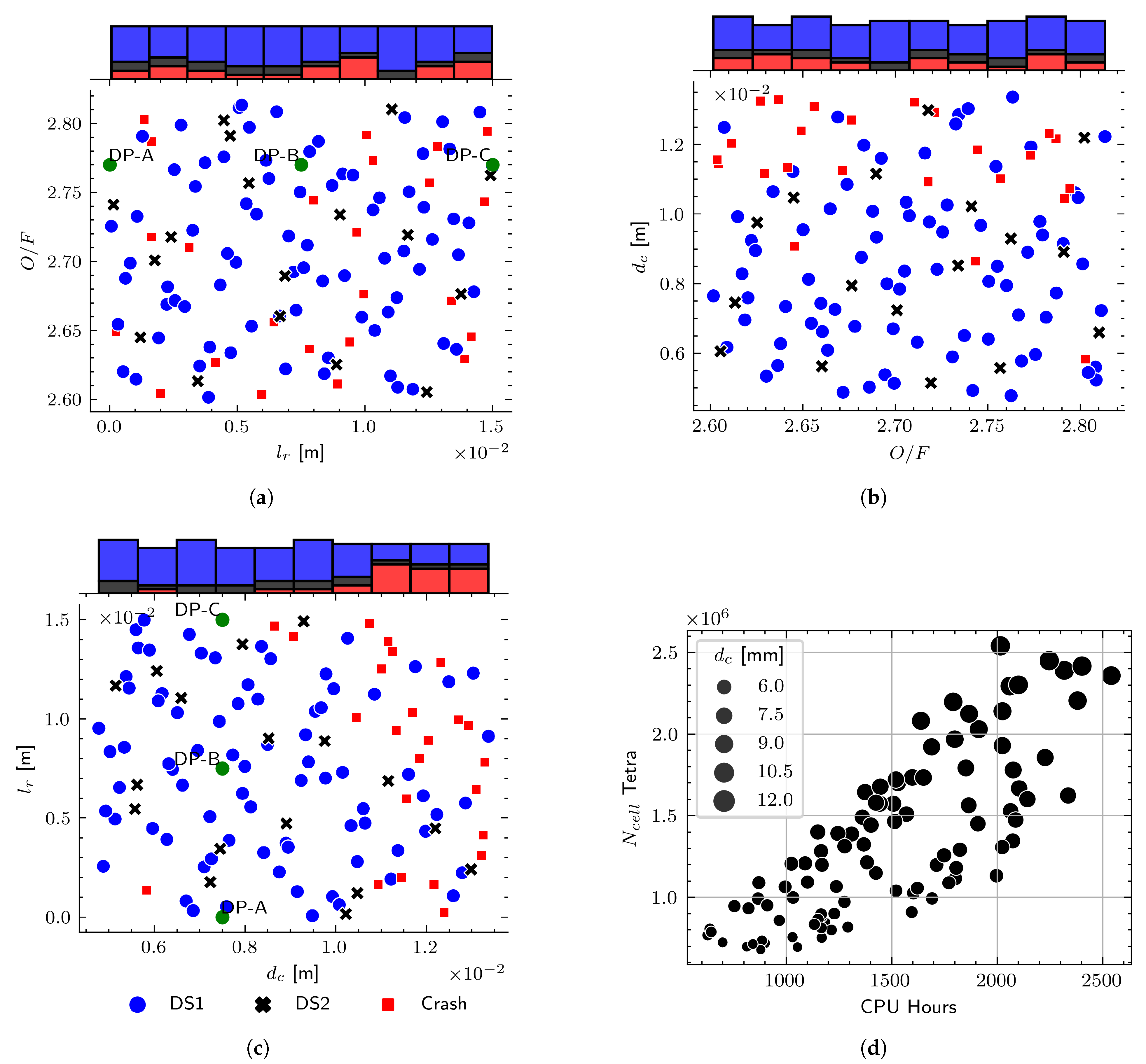
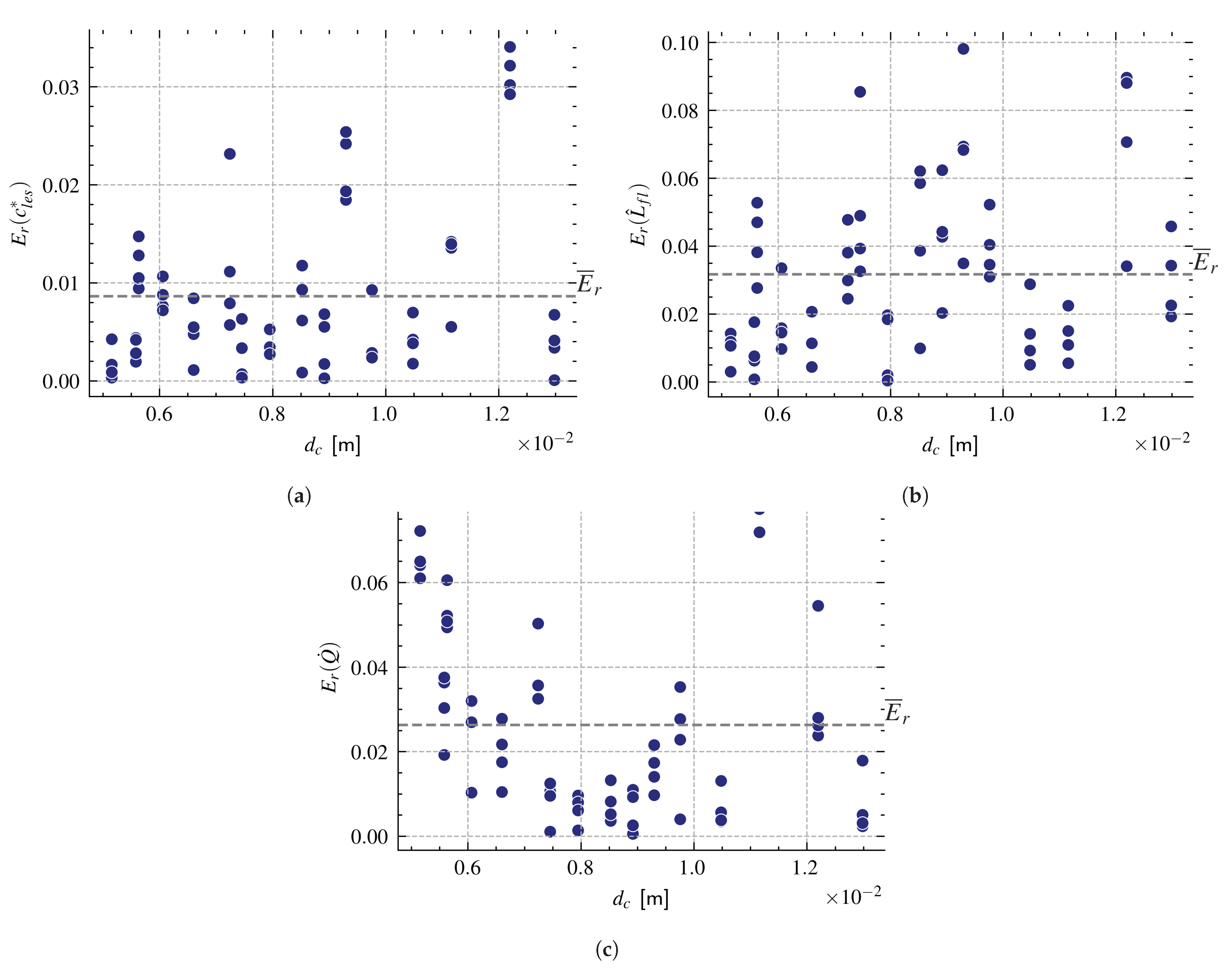
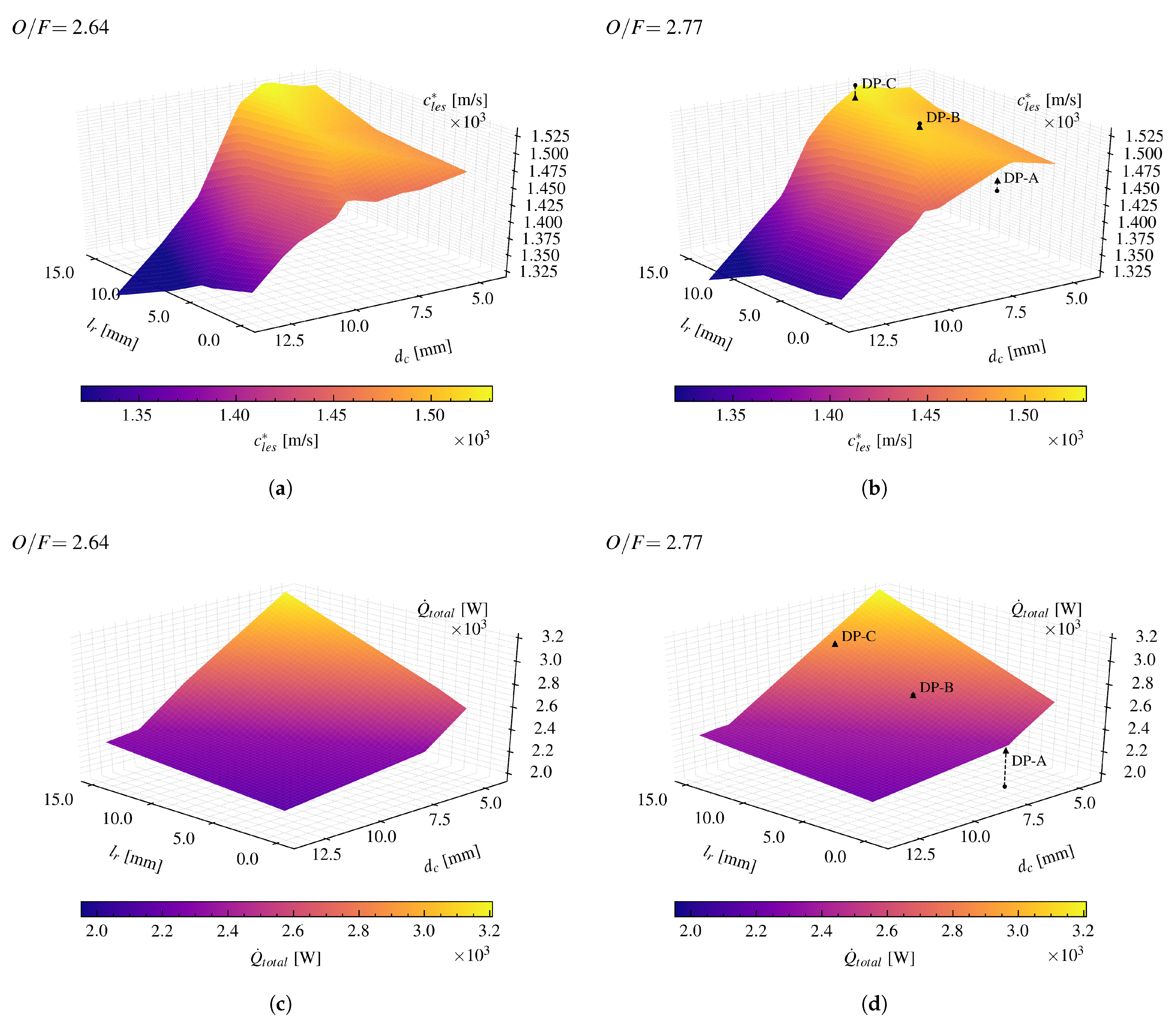
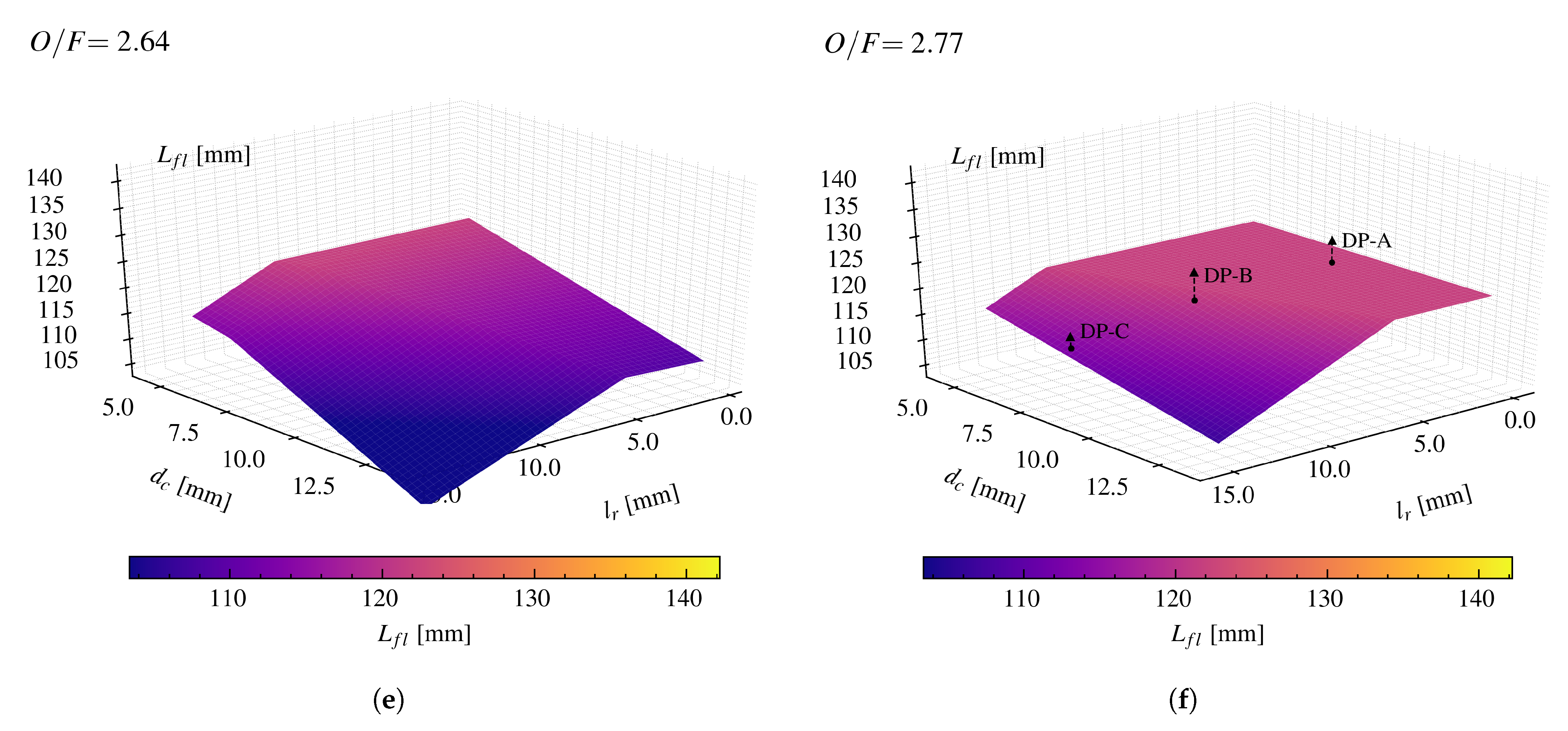
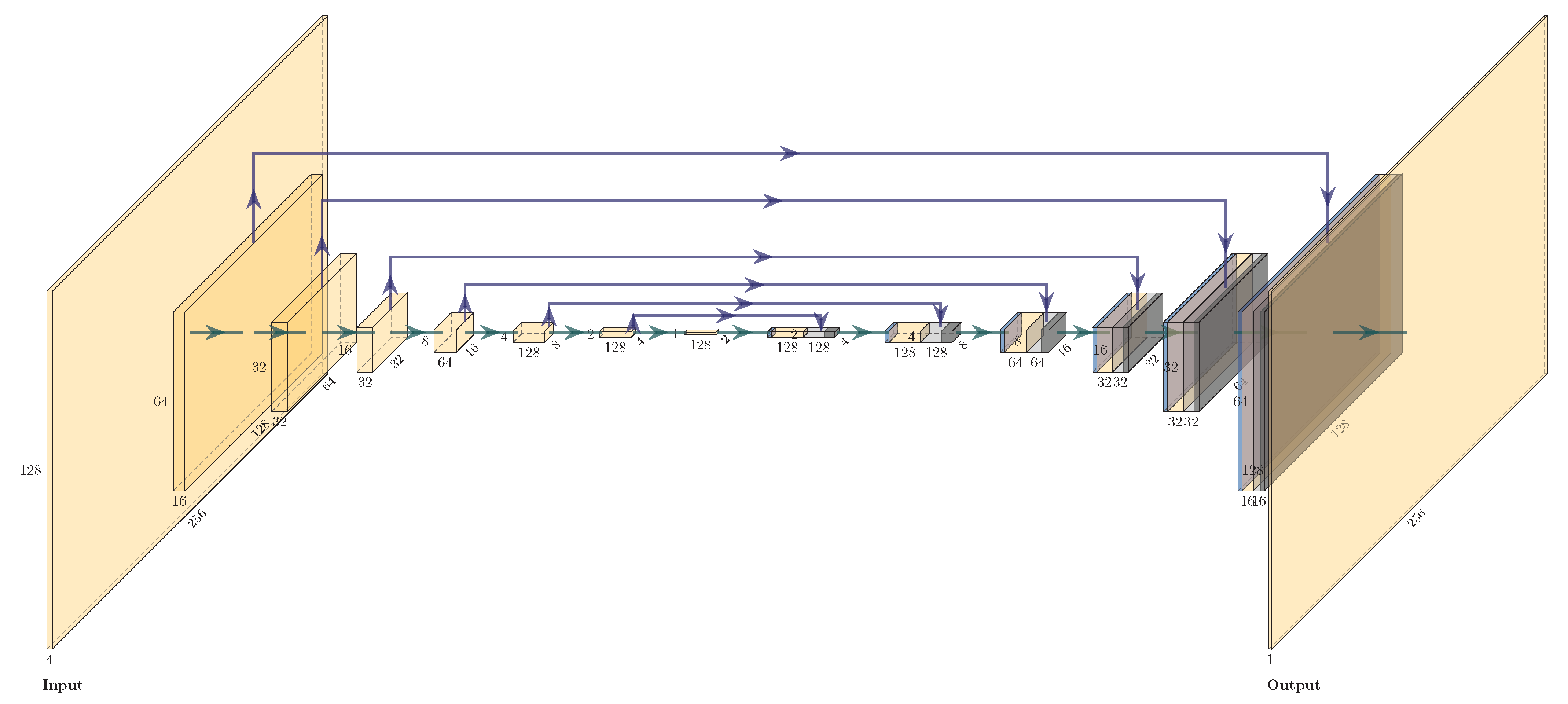
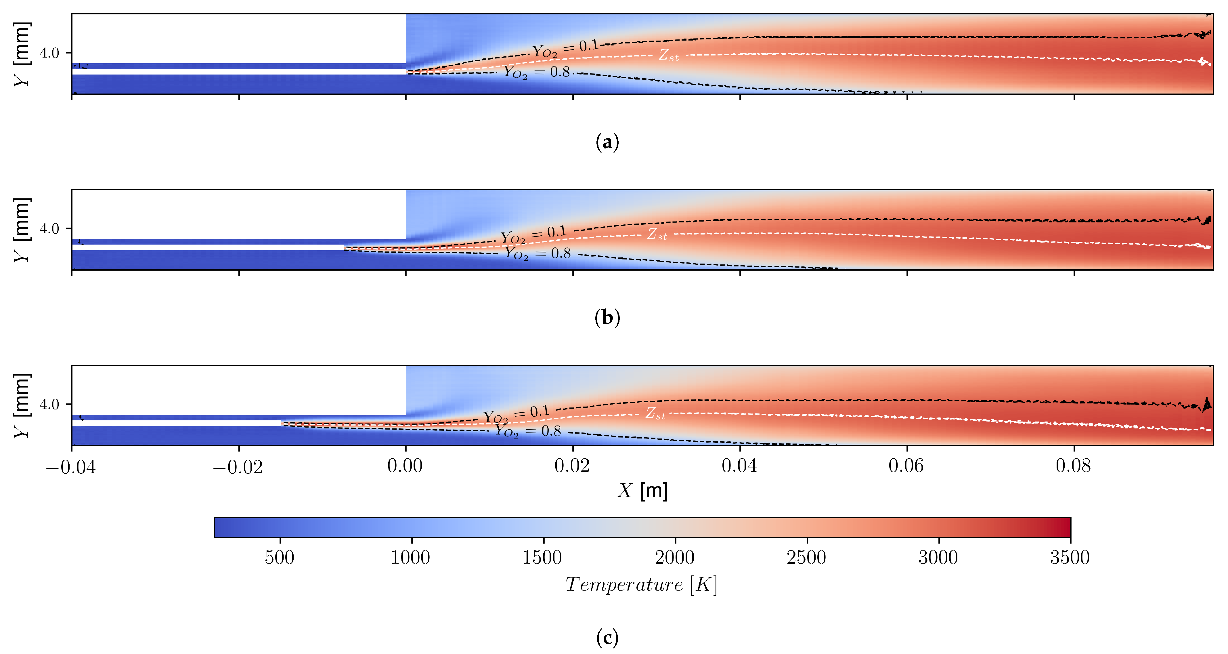
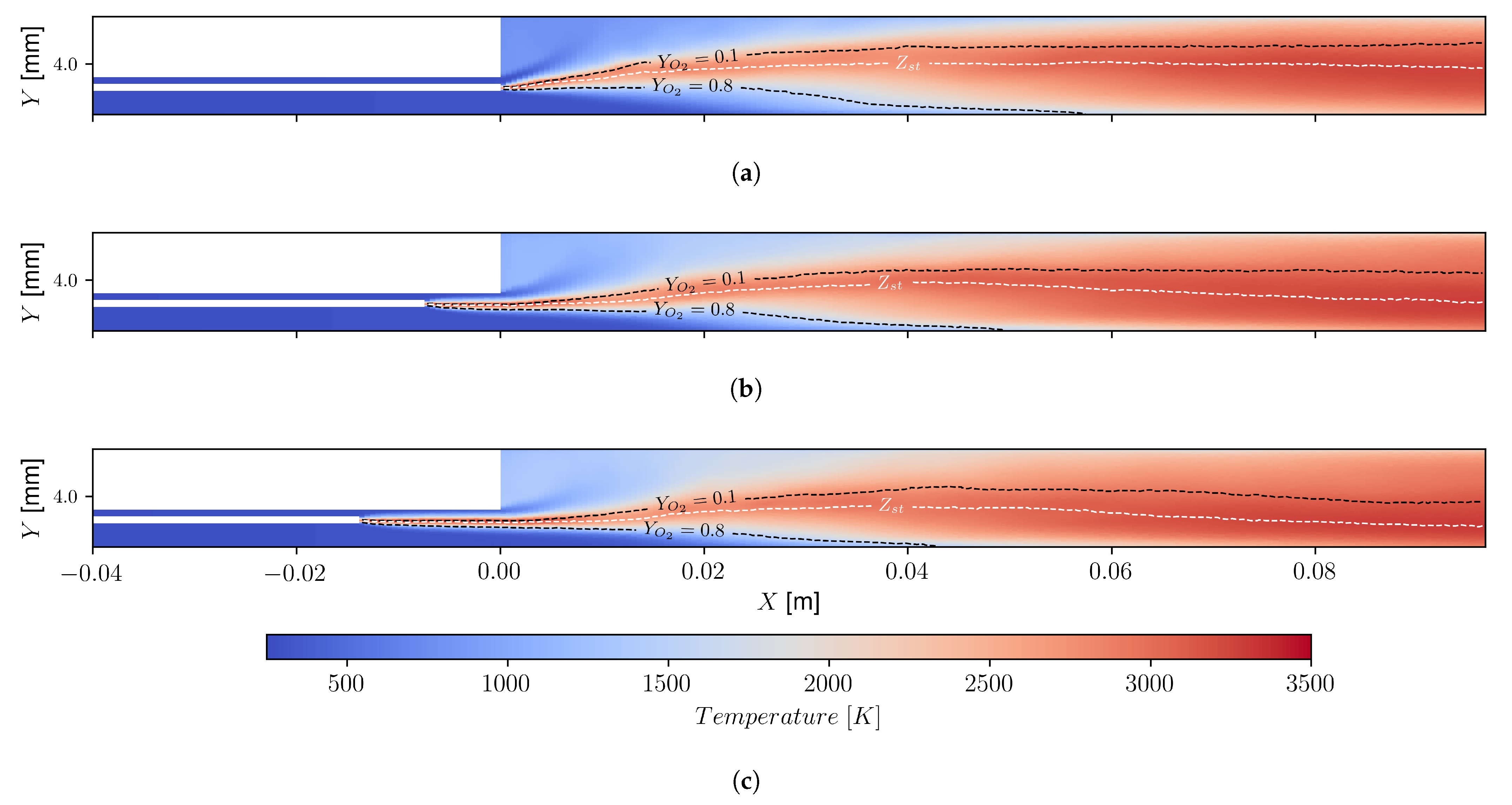
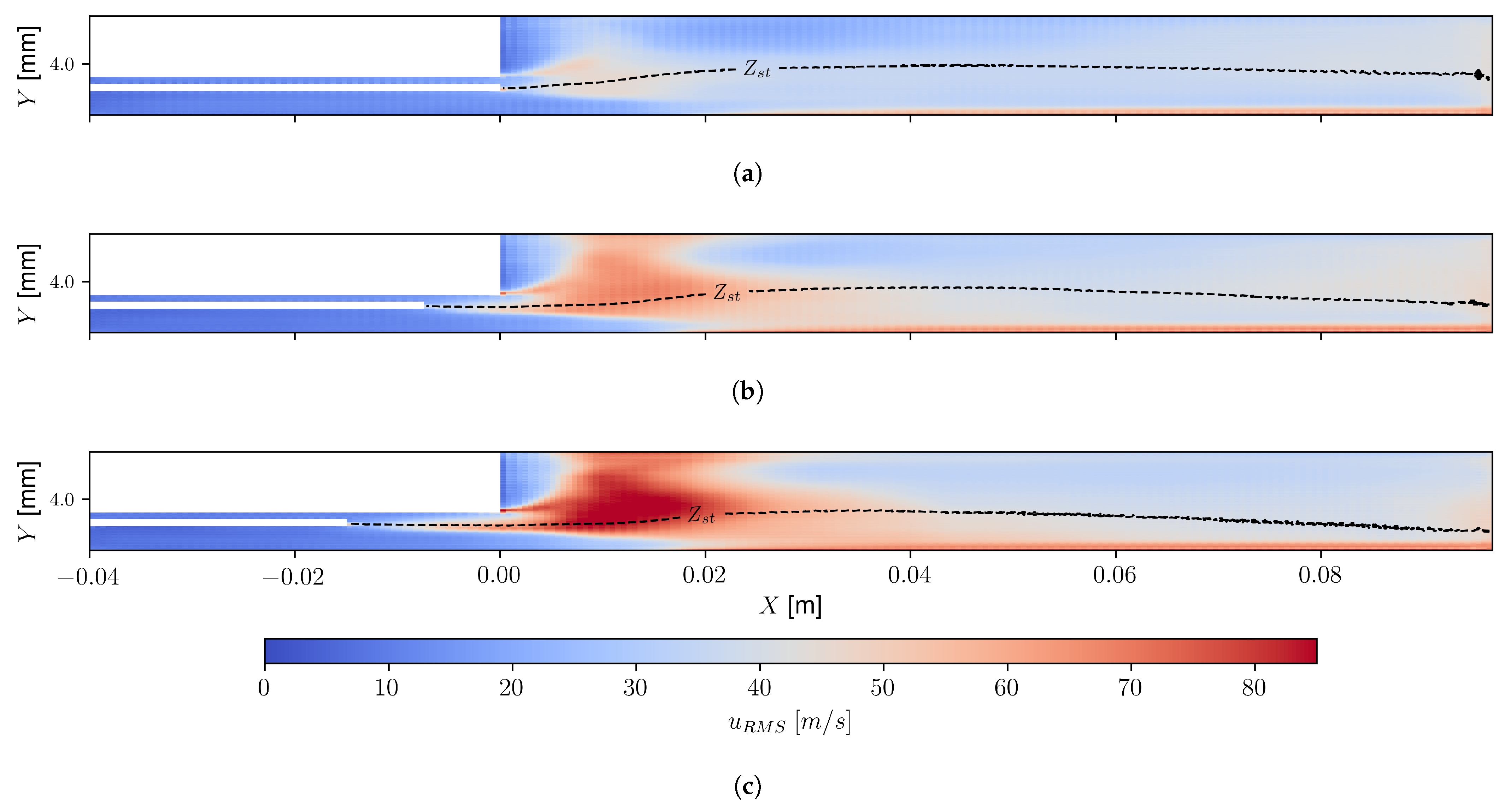
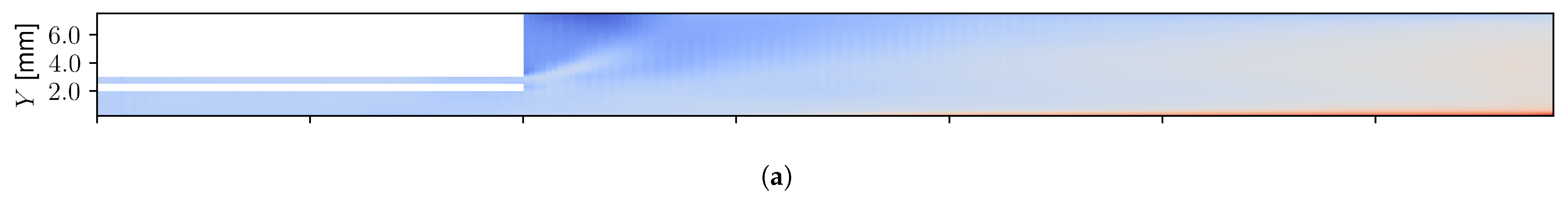
In the current work, the evolution of global quantities has been studied through the use of deep learning (DL)-based surrogate models. These quantities are the injectors’ characteristic velocity of the gases in the combustion chamber ($c_{les}^{*}$), the total wall heat-flux ($\dot{Q}$), and the approximate flame or combustion length (${\tilde{L}}_{fl}$). For such purposes, a database of $100$ LES simulations was built with AVBP by sampling a three-dimensional design-space. The axes considered were: the mixture ratio ($O/F$), the oxidizer post’s recess length ($l_r$), and the chamber radius ($d_c$). Furthermore, a methodology for deriving two-dimensional surrogate models of field quantities of interest has been put in place. The ultimate objective of these models is to provide interpretability to the behavior of the global quantities model over the design space. Surrogate models for the time-averaged temperature field ($\overline{T}$), velocity-u field ($\overline{u}$), oxygen mass fraction field (${\overline{Y}}_{O_2}$), mixture-fraction field ($\overline{\Xi }$), and velocity-u root mean-squared field ($u_{RMS}$) were obtained by means of U-Nets and isolated network hyperparameter optimization. The predictions given by these models give estimates of a longitudinal cut of the three-dimensional solution in a $256\times 128$ Cartesian grid. These networks have shown acceptable predictive performances in terms of the average test dataset’s relative and normalized errors.

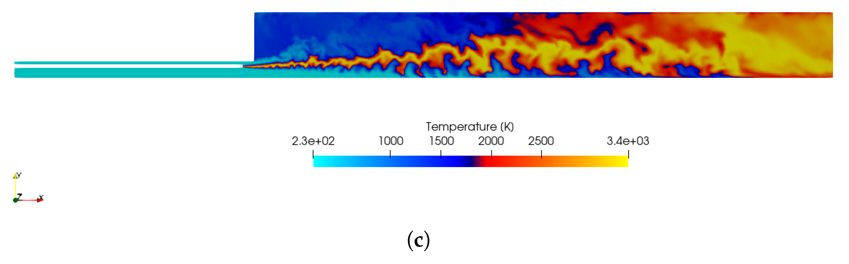
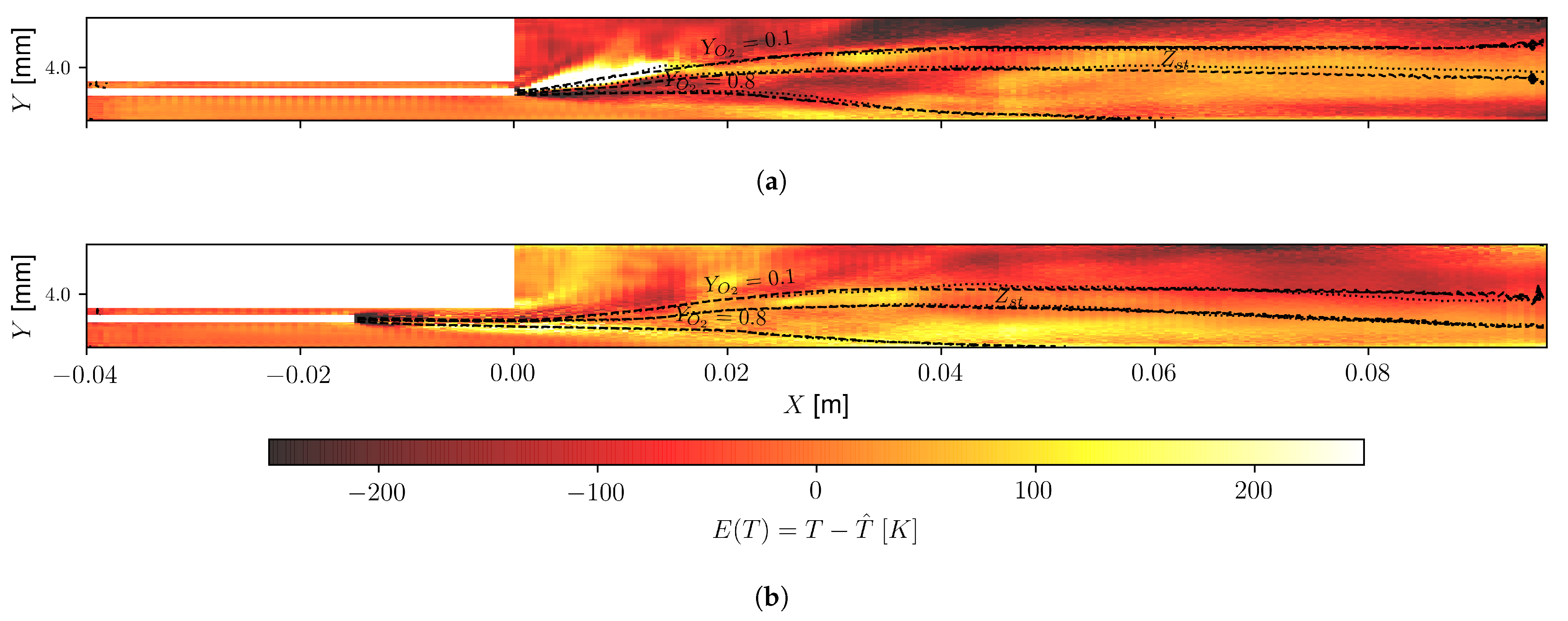
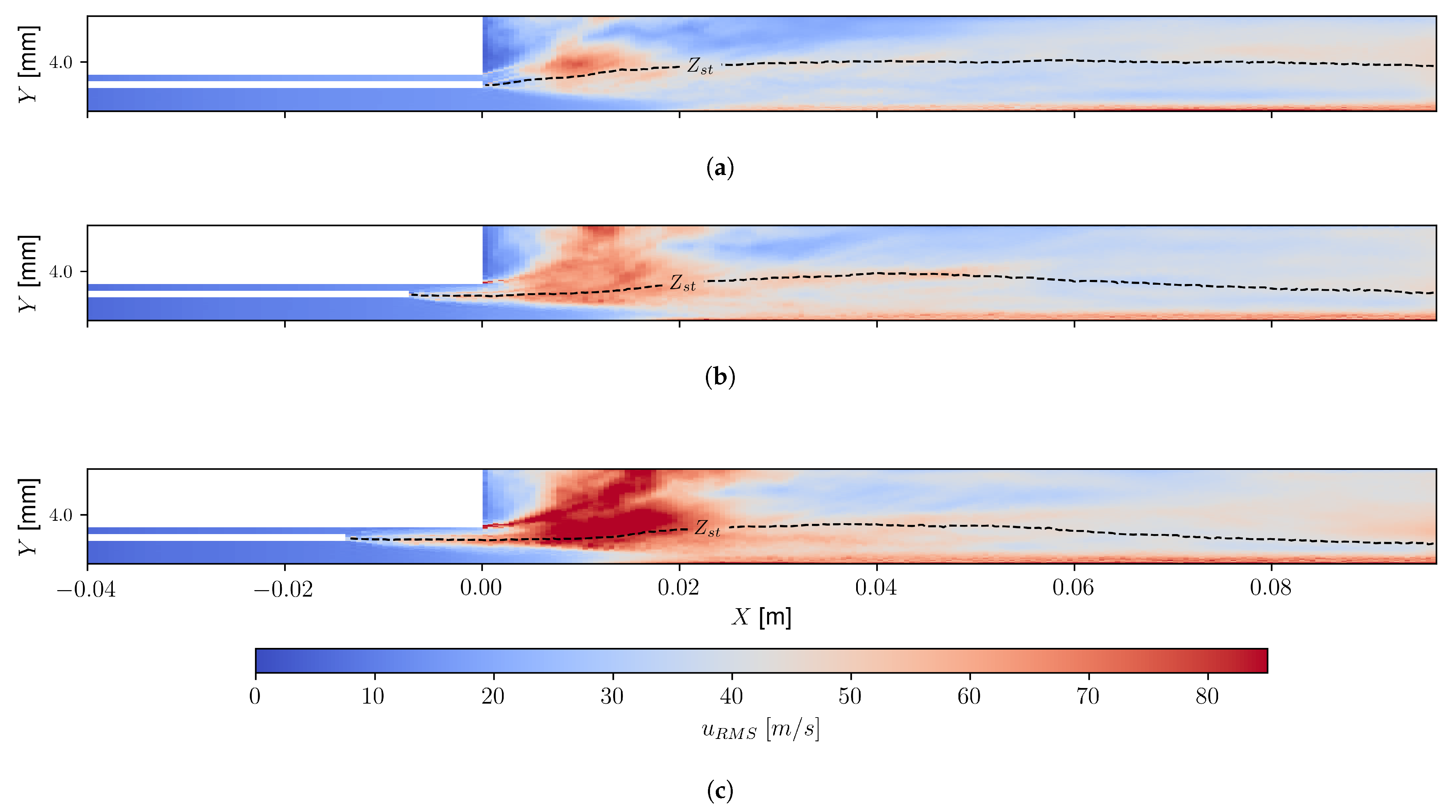
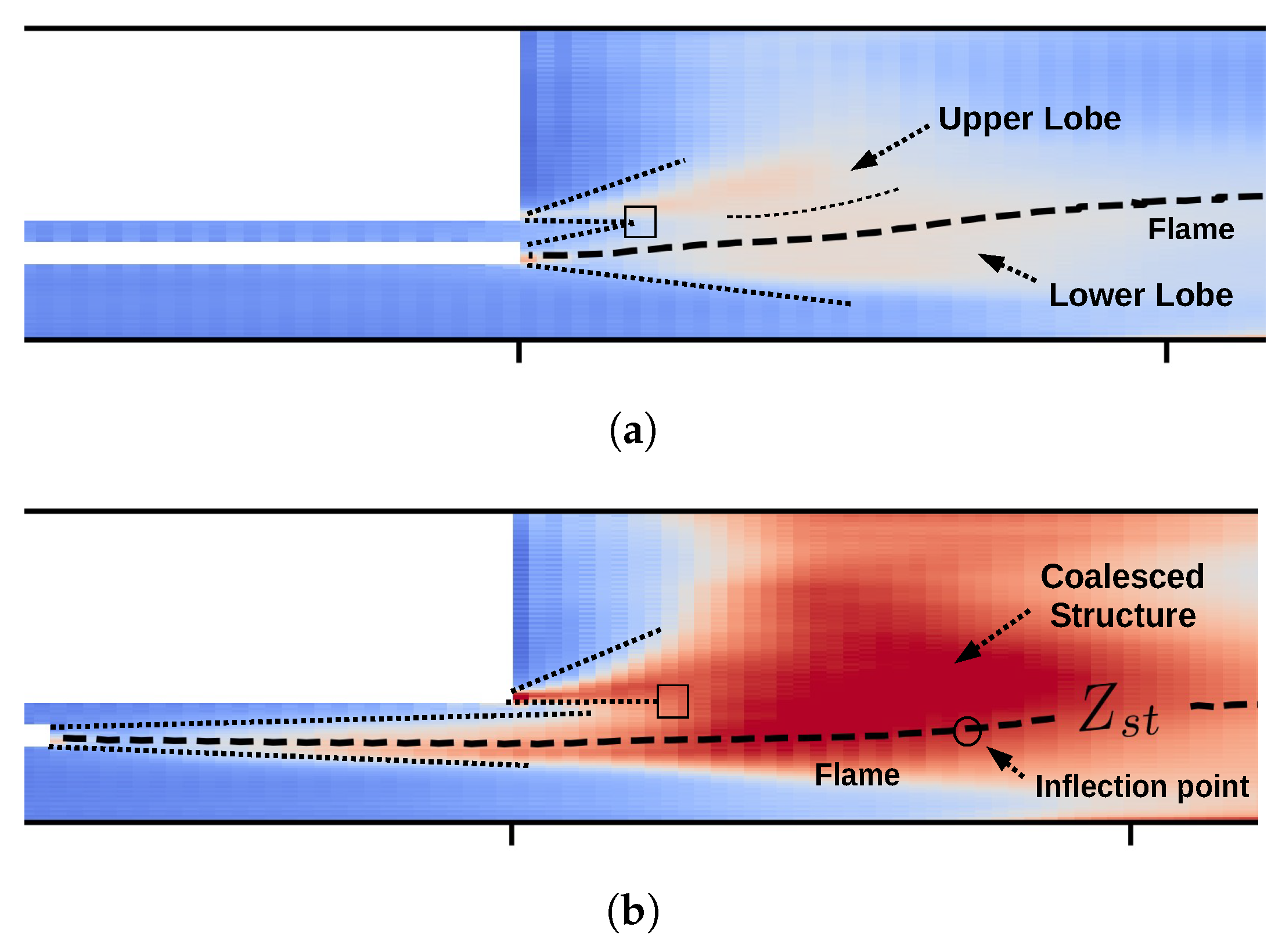
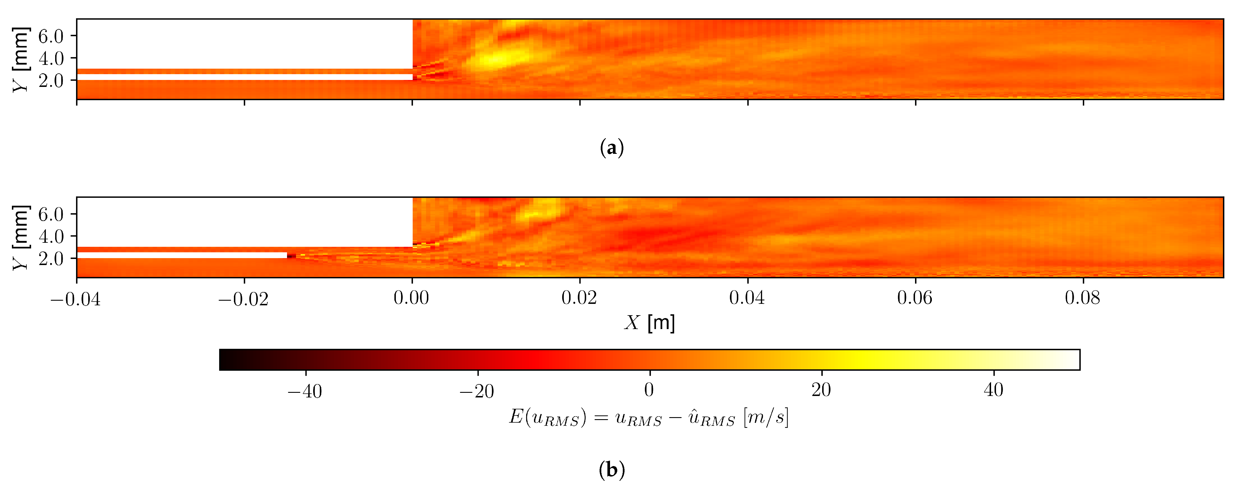
Special interest has been placed on the influences of the recess length on the considered quantities. Making use of the surrogate models to navigate the design space, we see that recessing the oxidizer post leads to an increase in $c_{les}^{*}$. It was observed from the analysis U-Nets’ outputs of different injector design points that higher temperatures are present in the recirculation zone, which is linked to a faster expansion of flame, a phenomenon that has been experimentally observed. Moreover, oxygen mass fraction iso-lines and the stoichiometric lines are displaced upstream with increasing values of recess, thereby hinting at a faster consumption rate. The topology of the error field shows good agreement for the temperature field, the oxygen mass fraction, and mixture fraction iso-lines. The larges differences can be observed in the vicinity of the stretched flame, where high gradients are also present. The analysis of the root mean squared (RMS) of velocity-u fluctuations shows a strong reaction to recess, with a clear increase in the fluctuations’ intensity in the vicinity of the flame sheet. The surrogate models resolve well most of the relevant structures of the $u_{RMS}$ field; however, detailed analysis of the error fields indicate that some are missing for the design points reviewed.

Finally, projected future works intend to continue the focus on the development of DL-based surrogate models to include the wall heat-flux profile and to improve the predictive performances of the field quantities models. Benchmarking against other DL-based data-driven techniques such as GNNs and MLPs is envisioned. The major conundrum lies in the elevated costs per sample for LES, which renders efforts to increase the fidelity or size of the database extremely expensive. Thus, subsequent efforts will be performed in order to increase the sampling efficacy.

References

1. Scheetz, M. Bank of America Expects the Space Industry to Triple to a $1.4 Trillion Market within a Decade. Available online: https://www.cnbc.com/2020/10/02/why-the-space-industry-may-triple-to-1point4-trillion-by-2030.html (accessed on 2 October 2020).
2. Scatteia, L. Main Trends and Challenges in the Space Sector. Available online: https://www.pwc.fr/fr/assets/files/pdf/2019/06/fr-pwc-main-trends-and-challenges-in-the-space-sector.pdf (accessed on 2 October 2020).
3. Sutton, G.P.; Biblarz, O. Rocket Propulsion Elements, 8th ed.; John Wiley and Sons, Inc.: Hoboken, NJ, USA, 2000. [Google Scholar]
4. Bouhlel, M.A.; Hwang, J.T.; Bartoli, N.; Lafage, R.; Morlier, J.; Martins, J.R. A Python Surrogate Modeling Framework with Derivatives. Adv. Eng. Softw. 2019, 135, 102662. [Google Scholar] [CrossRef] [Green Version]
5. Hwang, J.T.; Martins, J.R.R.A. A Fast-Prediction Surrogate Model for Large Datasets. Aerosp. Sci. Technol. 2018, 75, 74–87. [Google Scholar] [CrossRef]
6. Chen, L.; Cakal, B.; Hu, X.; Thuerey, N. Numerical Investigation of Minimum Drag Profiles in Laminar Flow Using Deep Learning Surrogates. J. Fluid Mech. 2021, 919, A34. [Google Scholar] [CrossRef]
7. Yu, J.; Hesthaven, J.S. Flowfield Reconstruction Method Using Artificial Neural Network. AIAA J. 2019, 57, 482–498. [Google Scholar] [CrossRef]
8. Wang, X.; Chang, Y.H.; Li, Y.; Yang, V.; Su, Y.H. Surrogate-based modeling for emulation of supercritical injector flow and combustion. Proc. Combust. Inst. 2021, 38, 6393–6401. [Google Scholar] [CrossRef]
9. White, C.; Ushizima, D.; Farhat, C. Fast Neural Network Predictions from Constrained Aerodynamics Datasets. arXiv 2019, arXiv:1902.00091. [Google Scholar]
10. Kontolati, K.; Loukrezis, D.; Santos, K.R.M.d.; Giovanis, D.G.; Shields, M.D. Manifold learning-based polynomial chaos expansions for high-dimensional surrogate models. Int. J. Uncertain. Quantif. 2022, 12, 39–64. [Google Scholar] [CrossRef]
11. Lee, K.; Carlberg, K.T. Model reduction of dynamical systems on nonlinear manifolds using deep convolutional autoencoders. J. Comput. Phys. 2020, 404, 108973. [Google Scholar] [CrossRef] [Green Version]
12. Vinuesa, R.; Brunton, S.L. The Potential of Machine Learning to Enhance Computational Fluid Dynamics. arXiv 2021, arXiv:2110.02085. [Google Scholar]
13. Fresca, S.; Dede’, L.; Manzoni, A. A Comprehensive Deep Learning-Based Approach to Reduced Order Modeling of Nonlinear Time-Dependent Parametrized PDEs. J. Sci. Comput. 2021, 87, 61. [Google Scholar] [CrossRef]
14. Fresca, S.; Manzoni, A. POD-DL-ROM: Enhancing deep learning-based reduced order models for nonlinear parametrized PDEs by proper orthogonal decomposition. Comput. Methods Appl. Mech. Eng. 2022, 388, 114181. [Google Scholar] [CrossRef]
15. Fries, W.D.; He, X.; Choi, Y. LaSDI: Parametric Latent Space Dynamics Identification. Comput. Methods Appl. Mech. Eng. 2022, 399, 115436. [Google Scholar] [CrossRef]
16. McQuarrie, S.A.; Huang, C.; Willcox, K.E. Data-Driven Reduced-Order Models Via Regularised Operator Inference for a Single-Injector Combustion Process. J. R. Soc. N. Z. 2021, 51, 194–211. [Google Scholar] [CrossRef]
17. Huang, C.; Duraisamy2, K.; Merkle3, C. Component-Based Reduced Order Modeling of Large-Scale Complex Systems. Front. Phys. 2022, 10, 900064. [Google Scholar] [CrossRef]
18. Swischuk, R.; Kramer, B.; Huang, C.; Willcox, K. Learning Physics-Based Reduced-Order Models for a Single-Injector Combustion Process. AIAA J. 2020, 58, 2658–2672. [Google Scholar] [CrossRef] [Green Version]
19. Huang, C.; Wentland, C.R.; Duraisamy, K.; Merkle, C. Model Reduction for Multi-Scale Transport Problems using Model-form Preserving Least-Squares Projections with Variable Transformation. arXiv 2021, arXiv:2011.02072. [Google Scholar] [CrossRef]
20. Hesthaven, J.; Ubbiali, S. Non-intrusive reduced order modeling of nonlinear problems using neural networks. J. Comput. Phys. 2018, 363, 55–78. [Google Scholar] [CrossRef] [Green Version]
21. Hasegawa, K.; Fukami, K.; Murata, T.; Fukagata, K. Machine-learning-based reduced-order modeling for unsteady flows around bluff bodies of various shapes. Theor. Comput. Fluid Dyn. 2020, 34, 367–383. [Google Scholar] [CrossRef]
22. Mondal, S.; Torelli, R.; Lusch, B.; Milan, P.J.; Magnotti, G.M. Accelerating the Generation of Static Coupling Injection Maps Using a Data-Driven Emulator. SAE Int. J. Adv. Curr. Pract. Mobil. 2021, 3, 1408–1424. [Google Scholar] [CrossRef]
23. Milan, P.J.; Torelli, R.; Lusch, B.; Magnotti, G.M. Data-driven model reduction of multiphase flow in a single-hole automotive injector. At. Sprays 2020, 30, 401–429. [Google Scholar] [CrossRef]
24. Shyy, W.; Tucker, P.K.; Vaidyanathan, R. Response Surface and Neural Network Techniques for Rocket Engine Injector Optimization. J. Propuls. Power 2001, 17, 391–401. [Google Scholar] [CrossRef]
25. Vaidyanathan, R.; Tucker, P.K.; Papila, N.; Shyy, W. Computational-Fluid-Dynamics-Based Design Optimization for Single-Element Rocket Injector. J. Propuls. Power 2004, 20, 705–717. [Google Scholar] [CrossRef]
26. Brunton, S.L.; Noack, B.R.; Koumoutsakos, P. Machine Learning for Fluid Mechanics. Annu. Rev. Fluid Mech. 2020, 52, 477–508. [Google Scholar] [CrossRef] [Green Version]
27. Cai, S.; Mao, Z.; Wang, Z.; Yin, M.; Karniadakis, G.E. Physics-informed neural networks (PINNs) for fluid mechanics: A review. arXiv 2021, arXiv:2105.09506. [Google Scholar] [CrossRef]
28. Farimani, A.B.; Gomes, J.; Pande, V.S. Deep Learning the Physics of Transport Phenomena. arXiv 2017, arXiv:1709.02432. [Google Scholar]
29. Guo, X.; Li, W.; Iorio, F. Convolutional Neural Networks for Steady Flow Approximation. In Proceedings of the 22nd ACM SIGKDD International Conference on Knowledge Discovery and Data Mining, San Francisco, CA, USA, 13–17 August 2016; ACM: San Francisco, CA, USA, 2016; pp. 481–490. [Google Scholar] [CrossRef]
30. Zhang, Y.; Sung, W.J.; Mavris, D. Application of Convolutional Neural Network to Predict Airfoil Lift Coefficient. arXiv 2018, arXiv:1712.10082. [Google Scholar]
31. Thuerey, N.; Weissenow, K.; Prantl, L.; Hu, X. Deep Learning Methods for Reynolds-Averaged Navier-Stokes Simulations of Airfoil Flows. AIAA J. 2020, 58, 25–36. [Google Scholar] [CrossRef]
32. Kim, B.; Azevedo, V.C.; Thuerey, N.; Kim, T.; Gross, M.; Solenthaler, B. Deep Fluids: A Generative Network for Parameterized Fluid Simulations. Comput. Graph. Forum 2019, 38, 59–70. [Google Scholar] [CrossRef] [Green Version]
33. Krügener, M.; Zapata Usandivaras, J.F.; Bauerheim, M.; Urbano, A. Coaxial-Injector Surrogate Modeling Based on Reynolds-Averaged Navier–Stokes Simulations Using Deep Learning. J. Propuls. Power 2022, 38, 783–798. [Google Scholar] [CrossRef]
34. Usandivaras, J.F.Z.; Krügener, M.; Urbano, A.; Bauerheim, M.; Cuenot, B. Data driven emulation models for Rocket Engines Injector design. In Proceedings of the IAC 2021—72nd International Astronautical Congress 2021, Dubai, United Arab Emirates, 25–29 October 2021. [Google Scholar]
35. Brunton, S.L. Applying Machine Learning to Study Fluid Mechanics. arXiv 2021, arXiv:2110.02083. [Google Scholar] [CrossRef]
36. Haidn, O.J. Advanced Rocket Engines. In Advances on Propulsion Technology for High-Speed Aircraft; Educational Notes RTO-EN-AVT-150, Paper 6; RTO: Neuilly-sur-Seine, France, 2008. [Google Scholar]
37. Villermaux, E.; Rehab, H. Mixing in coaxial jets. J. Fluid Mech. 2000, 425, 161–185. [Google Scholar] [CrossRef]
38. Tacina, K.M.; Dahm, W.J.A. Effects of heat release on turbulent shear flows. Part 1. A general equivalence principle for non-buoyant flows and its application to turbulent jet flames. J. Fluid Mech. 2000, 415, 23–44. [Google Scholar] [CrossRef]
39. Silvestri, S.; Winter, F.; Celano, M.P.; Schlieben, G.; Knab, O.; Haidn, O. Investigation on Recess Variation of a Shear Coax Injector in a GOX-GCH4 Rectangular Combustion Chamber with Optical Access. In Proceedings of the 7th European Conference for Aeronautics and Space Sciences, Milano, Italy, 3–6 July 2017. [Google Scholar] [CrossRef]
40. Lux, J.; Haidn, O. Effect of Recess in High-Pressure Liquid Oxygen/Methane Coaxial Injection and Combustion. J. Propuls. Power 2009, 25, 24–32. [Google Scholar] [CrossRef]
41. Kendrick, D.; Herding, G.; Scouflaire, P.; Rolon, C.; Candel, S. Effects of a Recess on Cryogenic Flame Stabilization. Combust. Flame 1999, 118, 327–339. [Google Scholar] [CrossRef]
42. Juniper, M.P.; Candel, S.M. The stability of ducted compound flows and consequences for the geometry of coaxial injectors. J. Fluid Mech. 2003, 482, 257–269. [Google Scholar] [CrossRef] [Green Version]
43. Schonfeld, T.; Rudgyard, M. Steady and Unsteady Flow Simulations Using the Hybrid Flow Solver AVBP. AIAA J. 1999, 37, 1378–1385. [Google Scholar] [CrossRef]
44. Poinsot, T.; Veynante, D. Theoretical and Numerical Combustion, 2nd ed.; Edwards: Philadelphia, PA, USA, 2005. [Google Scholar]
45. Celano, M.P.; Silvestri, S.; Schlieben, G.; Kirchberger, C.; Haidn, O.J.; Dawson, T.; Ranjan, R.; Menon, S. Numerical and Experimental Investigation for a GOX-GCH4 Shear-Coaxial Injector Element. In Proceedings of the Space Propulsion Conference 2014, Cologne, Germany, 19–22 May 2014; Number SP2014-2969417. [Google Scholar]
46. Perakis, N.; Celano, M.P.; Haidn, O.J. Heat flux and temperature evaluation in a rectangular multi-element GOX/GCH4 combustion chamber using an inverse heat conduction method. In Proceedings of the 7th European Conference for Aeronautics and Aerospace Sciences (EUCASS), Milan, Italy, 3–6 July 2017; p. 15. [Google Scholar]
47. Maestro, D.; Cuenot, B.; Selle, L. Large Eddy Simulation of Combustion and Heat Transfer in a Single Element GCH 4/GOx Rocket Combustor. Flow Turbul. Combust. 2019, 103, 699–730. [Google Scholar] [CrossRef]
48. Poinsot, T.; Lelef, S. Boundary conditions for direct simulations of compressible viscous flows. J. Comput. Phys. 1992, 101, 104–129. [Google Scholar] [CrossRef]
49. Daviller, G.; Oztarlik, G.; Poinsot, T. A generalized non-reflecting inlet boundary condition for steady and forced compressible flows with injection of vortical and acoustic waves. Comput. Fluids 2019, 190, 503–513. [Google Scholar] [CrossRef] [Green Version]
50. Van Driest, E.R. Turbulent boundary layer in compressible fluids. J. Aeronaut. Sci. 1951, 18, 145–160. [Google Scholar] [CrossRef]
51. Lax, P.; Wendroff, B. Systems of conservation laws. Commun. Pure Appl. Math. 1960, 13, 217–237. [Google Scholar] [CrossRef] [Green Version]
52. Nicoud, F.; Toda, H.B.; Cabrit, O.; Bose, S.; Lee, J. Using singular values to build a subgrid-scale model for large eddy simulations. Phys. Fluids 2011, 23, 085106. [Google Scholar] [CrossRef]
53. Blanchard, S.; Cazères, Q.; Cuenot, B. Chemical modeling for methane oxy-combustion in Liquid Rocket Engines. Acta Astronaut. 2022, 190, 98–111. [Google Scholar] [CrossRef]
54. Alexander Schumaker, S.; Driscoll, J.F. Mixing properties of coaxial jets with large velocity ratios and large inverse density ratios. Phys. Fluids 2012, 24, 055101. [Google Scholar] [CrossRef]
55. Ruiz, A. Unsteady Numerical Simulations of Transcritical Turbulent Combustion in Liquid Rocket Engines. Ph.D. Thesis, Institut National Polytechnique de Toulouse—INPT, Toulouse, France, 1992. [Google Scholar]
56. McKay, M.D.; Beckman, R.J.; Conover, W.J. A Comparison of Three Methods for Selecting Values of Input Variables in the Analysis of Output from a Computer Code. Technometrics 1979, 21, 239–245. [Google Scholar]
57. Jin, R.; Chen, W.; Sudjianto, A. An efficient algorithm for constructing optimal design of computer experiments. J. Stat. Plan. Inference 2005, 134, 268–287. [Google Scholar] [CrossRef]
58. Paszke, A.; Gross, S.; Massa, F.; Lerer, A.; Bradbury, J.; Chanan, G.; Killeen, T.; Lin, Z.; Gimelshein, N.; Antiga, L.; et al. PyTorch: An Imperative Style, High-Performance Deep Learning Library. In Proceedings of the 33rd Conference on Neural Information Processing Systems (NeurIPS 2019), Vancouver, BC, Canada, 8–14 December 2019; p. 12. [Google Scholar]
59. Biewald, L. Experiment Tracking with Weights and Biases. 2020. Available online: https://docs.wandb.ai/company/academics (accessed on 2 October 2022).
60. Ronneberger, O.; Fischer, P.; Brox, T. U-Net: Convolutional Networks for Biomedical Image Segmentation. In Medical Image Computing and Computer-Assisted Intervention—MICCAI 2015; Lecture Notes in Computer Science; Navab, N., Hornegger, J., Wells, W.M., Frangi, A.F., Eds.; Springer International Publishing: Cham, Switzerland, 2015; Volume 9351, pp. 234–241. [Google Scholar] [CrossRef]
61. Usandivaras, J.F.Z.; Urbano, A.; Bauerheim, M.; Cuenot, B. Large Eddy Simulations and Deep Learning for the investigation of recess variation of a shear-coaxial injector. In Proceedings of the Space Propulsion Conference, Estoril, Portugal, 9–13 May 2022. Number SP2022-246. [Google Scholar]
Figure 1. Schematic of a coaxial-jet structure for a recessed injector with recess length l r . Inner and outer mixing-layers are formed between the central and annular flow, and the annular and external environment, respectively.
Aerospace 09 00594 g001
Figure 2. (a) Schematic of the geometry of the shear-coaxial injector used; key geometry parameters are specified. The fuel and oxidizer inlet channels and the outlet are identified; all adiabatic-slip walls are colored in black. (b) Three-dimensional view (3D) of a representative domain used in the confection of the LES database of shear-coaxial injectors. (c) Longitudinal cut of the instantaneous temperature field of one sample from the LES dataset of shear-coaxial injectors. Corresponding values are: lr = 1.92 mm, dc = 11.22 mm, and O/F = 2.445.
Aerospace 09 00594 g002aAerospace 09 00594 g002b
Figure 3. Joint plots of the points from the DOE projected in two-dimensional subspaces and consumption statistics graph. Colored histograms of the abscissa are displayed on top. (a) l r vs. O / F , (b) O / F vs. d c , (c) d c vs. l r , and (d) CPU hours consumed vs. number of tetrahedral cells in mesh used. The locations of DP-A, DP-B, and DP-C introduced later in Section 5, have been included as green dots for reference in (a,c).
Aerospace 09 00594 g003
Figure 4. Scatter plots of the relative errors of the best-performing networks, for every fold and sample of DS2 as a function of the sample dc coordinate of each of the global quantities: (a) c l e s * , (b) L ^ f l , and (c) Q ˙ . The average error across samples and folds is highlighted in gray for every plot.
Aerospace 09 00594 g004
Figure 5. Design space navigation charts for global quantities: (a,b) c l e s * , (c,d) Q ˙ , and (e,f) L ˜ f l obtained with the FCNNs indicated in Table 3 at mixture ratios ( O / F ) of 2.64 and 2.77. The l r and d c axis limits are those fixed for the DOE. In (b,d,f), ground truth LES values are marked by • and the FCNN prediction by ▴. Their corresponding ground truth LES and FCNN are included in Table 6 for completeness.
Aerospace 09 00594 g005aAerospace 09 00594 g005b
Figure 6. Proposed U-Net architecture with Leaky ReLU activation functions, batch normalization, upsampling layers, and skip connections. The inputs consisted of a tensor with 4 channels, each of 128 × 256, and the output was a single channel of 128 × 256.
Aerospace 09 00594 g006
Figure 7. Scatter plot of the relative errors of the best-performing networks, for every fold and sample of DS2, as a function of the sample’s dc coordinate for each of the field quantities: (a) T ¯ , (b) Y ¯ O 2 , (c) Ξ ¯ , (d) u ¯ , and (e) uRMS. The average error across samples and folds is highlighted in gray for every plot.
Aerospace 09 00594 g007
Figure 8. Surrogate model predictions of T ¯ field. The Y ¯ O 2 [ 0.1 , 0.8 ] , Ξ ¯ = Z s t = 0.2 iso-lines have been included, as given by their corresponding models. (a) DP-A, (b) DP-B, and (c) DP-C evaluations. The aspect ratio of the figures was modified purposely to facilitate their scrutiny.
Aerospace 09 00594 g008
Figure 9. Ground-truth LES average temperature field interpolated into a 256 × 128 Cartesian grid. The Y O 2 ∈ [0.1, 0.8], Zst = 0.2 iso-lines have been overlaid for convenience. (a) DP-A, (b) DP-B, and (c) DP-C. The aspect ratio of the figures has been modified purposely to facilitate their scrutiny.
Aerospace 09 00594 g009
Figure 10. Predictive error in T ¯ field of the U-Net with respect to LES-interpolated data. Predicted and ground-truth lines are shown in dashed and dotted patterns, respectively. (a) DP-A and (b) DP-C. The color-scale has been deliberately saturated to (−250 K, 250 K) to better distinguish regions with prediction errors. For reference, 250 K is ~7.5% of the O2-CH4 adiabatic flame’s temperature. The aspect ratio of the figures has been modified purposely to facilitate their scrutiny.
Aerospace 09 00594 g010
Figure 11. uRMS model’s prediction for: (a) DP-A, (b) DP-B, and (c) DP-C. The stoichiometric line, denoted by Zst, as estimated by Ξ ¯ , has been overlaid on top. The aspect ratio of the figures has been modified purposely to facilitate their scrutiny.
Aerospace 09 00594 g011
Figure 12. Ground truth LES uRMS field interpolated into a 256 × 128 Cartesian grid. (a) DP-A, (b) DP-B, and (c) DP-C. The stoichiometric line, denoted by Zst, has been overlaid on top. The aspect ratio of the figures has been modified purposely to facilitate their scrutiny.
Aerospace 09 00594 g012
Figure 13. Close up view of uRMS in the near field of the jet for (a) DP-A and (b) DP-C. Both upper and inner-shear layers are denoted by thin dotted lines, whereas the flame location is indicated in thick dashed lines. In (a), the upper and lower lobes of mild fluctuations are identified. For (b) the approximate location of the inflection point in the stoichiometric line is signaled by ○. The position where upper and fuel-rich inner shear-layers commingle is indicated by ☐.
Aerospace 09 00594 g013
Figure 14. Predictive error of uRMS surrogate model with respect to the uRMS field from LES interpolated data. (a) DP-A and (b) DP-C. The color-scale has been deliberately saturated to (−50 m/s, 50 m/s) to better distinguish regions with prediction errors. The aspect ratio of the figures has been modified purposely to facilitate their scrutiny.
Aerospace 09 00594 g014
Figure 15. Velocity-u (axial component) field as given by the corresponding u ¯ U-Net. (a) DP-A and (b) DP-C. The aspect ratio of the figures has been modified purposely to facilitate their scrutiny.
Aerospace 09 00594 g015aAerospace 09 00594 g015b