Investigation and Improvement of T-Tail Junction Flow Separation for a Demonstration Aircraft

Abstract

Flow separation is easily induced at the junctions of aircraft components, and for aircraft with T-type tails, in particular, it can lead to loss of directional stability under a small sideslip angle. In the reported study, improved delayed detached eddy simulation with a shear-layer-adapted length scale based on the k–ω shear-stress transport method was used to analyze and rectify the corner separation at the junctions of the horizontal and vertical parts of the tail of a demonstration aircraft. This was done to (i) suppress the flow separation caused by the complex interaction of the boundary layers on the horizontal and vertical tail parts at their junctions, and (ii) prevent the vertical tail parts from having any separated flow on their pressure and suction sides. The results showed that the main cause of the loss of directional stability was separation flow on the suction sides of the vertical tail parts. The corner flow separation was suppressed significantly by only using fairing cones at the junctions of the horizontal and vertical tail parts, thereby allowing the aircraft to maintain directional stability under a small sideslip angle.

1. Introduction

Junction flows (JFs) are common, such as those on bridges, buildings, wings, submarines, turbines, compressors, and the radiators of electronic equipment. Such corner flow is due to the complex three-dimensional (3D) separated flow caused by the upstream boundary layer (BL) colliding with an obstacle, usually one that is protruding from an attached plane. Occurring with both blunt and streamlined obstacles, this phenomenon is due to the sudden change in pressure gradient caused by the obstacle and the 3D effects caused by the separation of horseshoe vortices [1]. Except at very low Reynolds numbers, and both laminar and turbulent BLs, JFs are triggered easily in a very wide range of Reynolds numbers [1].

For aircraft, JFs generally occur at the junctions of (i) wings and body, (ii) nacelles and wings, and (iii) horizontal and vertical tail parts, among other components. Once a JFs exists, the flow in the corner region oscillates and flaps the connecting components, which may threaten aircraft safety. JFs also produce additional interference drag that affects aerodynamic performance and even aircraft stability in the longitudinal and transverse directions [1]. Therefore, the flow mechanism for a separated flow in a junction area must be well understood, with this being very important for designing junctions such as wing–body, nacelle–wing, and horizontal–vertical tail junctions. For laminar-flow aircraft in particular, the airfoils used for the wings and horizontal and vertical tail parts have a small leading-edge radius, and the position of maximum thickness is relatively far back, thereby making flow separation in junction areas more likely [2].

The flow interference in a wing–body junction is actually caused by the fuselage and wing BLs intersecting at the junction, and because of the mutual fusion and interference of the BLs on both sides, the flow at the junction is highly anisotropic and very unsteady [1,2]. In addition, this physical phenomenon changes greatly with the flight state, wing leading-edge radius, and other factors, so the flow caused by the mutual BL interference is very complex [3]. Therefore, a better understanding of the flow mechanism for this mutual BL interference would greatly help in aircraft design and improve aircraft aerodynamic performance.

To date, the research on flows in junction areas has mainly been focused on the spatial separation point, bimodal instability, horseshoe-vortex oscillation, and other flow characteristics near the leading edge [2], and early JF research was mostly experimental in nature. Devenport and Simpson [4] conducted wind-tunnel experiments on a NACA0020 wing with a 3:2 elliptical leading edge, and other experiments showed that the generation and shedding of horseshoe vortices at the leading edge of an aircraft wing at the bottom of the corner area led to low-frequency oscillation in the leading-edge area of the wing [5]. By measuring the velocity in the leading-edge region and the wake, Fleming et al. [6] studied the span-wise flow velocity pattern caused by the transverse reverse pressure gradient. To study the anisotropy of near-wall turbulence, various researchers measured the strong cross flow at the stagnation point [7,8,9,10,11].

In comparison, there has been relatively little research on corner separated flows at the trailing edges of junction regions. Gand et al. [12] carried out a series of experiments and found that with an increase of Reynold number, the corner separation increases as well. Thus, this phenomenon involved in the flow at the junction between a wing and an aircraft body or a nacelle pylon can very commonly trigger a separation flow and thus impair the aerodynamics of the aircraft through so-called interference drag, which is estimated to constitute 10% of the total drag of a civil aircraft [2]. Baber [13] carried out a series of experiments to study the impact of an incoming BL on the corner separation, and the research showed that a thinner incoming boundary may cause a larger corner separation at the tailing edge. Jing et al. [14] experimented to invest the static directional stability (SDS) contribution of the vertical tail of a conventional aircraft, and they found a SDS loss at the vertical tail and body junction region because of corner separation. From the above research, it appears that junction corner separation might cause directional static instability of an aircraft when it occurs in the region of a T-tail. It is therefore important to understand the mechanisms involved in junction flow, especially for industrial configurations, where corner separation is among the most critical matters [15]. However, an incoming BL is affected by the leading edge of the wing and merges with the disturbed BL of the wing itself in the corner region. This simultaneous presence of two BLs and their merger in the junction region makes the flow in this region very complex and highly anisotropic. To date, corner separation flow represents one of the few remaining challenging issues in applied aerodynamics, and the design of belly fairings mostly relies on the designer’s experience [15].

The corner separated flow generated by the mutual interference of two BLs is the second kind of Prandtl secondary flow [1], and it is strongly anisotropy. For general Reynolds-averaged Navier–Stokes (RANS) methods, especially the Spalart–Allmaras (SA) and shear-stress transport (SST) methods and other commonly used methods based on linear eddy viscosity, although the flow solution has good accuracy outside the interference region, it is almost impossible to obtain ideal results in the influence range of the horseshoe–vortex system, especially in the separation region.

Due to the lack of nonlinear terms, the obtained separation region differs greatly from that obtained experimentally; this is the case even for the SST model, which is relatively good at capturing other flow details. Indeed, the deviations in separation size and position can be as large as 100% [2]. Apsley and Leschziner [16] used 12 turbulence models to simulate a wing/body junction numerically; although the results given by the two-equation SST model and the one-equation SA model were better than those given by the other models, all 12 turbulence models used in the calculation failed to capture well the separation position and size, and some models even failed to capture well the leading-edge saddle point and horseshoe–vortex structure. Parneix et al. [17] used the V2F model to simulate wing–body corner flow; this captured the 3D separation line and the leading-edge horseshoe vortex and its intensity, but it failed to successfully capture the separation flow in the junction area. Lien et al. [18] developed the improved the V2F method to calculate wing–body corner separation, but although the separation was captured successfully, the correct separation position and size were not.

Owing to the current lack of a deep understanding of flow separation in junction areas and the insufficient capture accuracy of the commonly used turbulence models based on linear eddy viscosity, since 2016 NASA has been carrying out a series of studies on the corner separated flow at the trailing edge caused by wing–body interference [19,20,21,22,23]. The aims are to (i) study the flow characteristics in the corner area, and (ii) form another standard calculation example for computational fluid dynamics (CFD), to assess the solution accuracy of CFD technology. In particular, experiments are carried out on flow details such as Reynolds stress, which allows greater evaluation of CFD calculation methods and offers a clearer direction for improving them.

To explore how separated flows in junction areas influence the SDS of a demonstration aircraft and improved design methods, this paper begins by introducing the complexity of flow in a junction area and the deficiency of the RANS methods, which are more mature in engineering applications at this stage. In Section 2, the shear-layer-adapted improved delayed detached eddy simulation (SLA-IDDES) method is briefly introduced, and then the standard Rood model is calculated using SLA-IDDES and compared with experimental results, to verify the accuracy of the flow simulated in the junction area. In Section 3, the SLA-IDDES method is used to perform calculations for a demonstration aircraft at a small angle of attack and different sideslip angles, and the results are compared with those from a wind-tunnel experiment, to verify the reliability of the method and speculate about the causes of the loss of SDS. In Section 4, the flow in the flat–vertical tail junction area of the demonstration aircraft is controlled via a rectifier cone, to inhibit the flow separation in the junction area, so as to analyze the specific causes of the loss of SDS and provide improvement measures.

2. Numerical Methodology

2.1. SLA Subgrid Model and Its Implementation in IDDES

To deal with the log-layer mismatch phenomenon that usually occurs in detached eddy simulation (DES) models, Shur et al. [24] developed the IDDES method through further improvement of delayed DES (DDES). Compared to the DES/DDES model, IDDES provides shielding against grid-induced separation and allows the model to run in wall-modelled large-eddy simulation (WMLES) mode, thereby making it possible to simulate unsteady modes of near-wall BLs.

In the original DES method, the subgrid length scale was considered to be too conservative to capture the Kelvin–Helmholtz instability in the near-wall region, and so Shur et al. [25] defined a new subgrid length scale, which for a hexahedral grid is given as

$${\tilde{\mathsf{\Delta }}}_{\omega }=\frac{1}{\sqrt{3}}\underset{n,m=1,\dots ,8}{\max }\left|I_n-I_m\right|$$

(1)

Here, we have $I_n=n_{\omega }\times r_n$, where $n_{\omega }$ is the unit vector aligned with the vorticity vector, and $r_n$ is the vector from vertex n to the center of the grid cell. According to Shur et al. [24], the change from ${\mathsf{\Delta }}_{\max }$ to ${\tilde{\mathsf{\Delta }}}_{\omega }$ alone may still be insufficient when the grid is not fine enough in the x and y directions to resolve the Kelvin–Helmholtz instability. Therefore, to make ${\tilde{\mathsf{\Delta }}}_{\omega }$ more effective, the empirical function

$$F_{\mathrm{KH}}(\langle \mathrm{VTM}\rangle )=\max \left\{F_{\mathrm{KH}}^{\min },\min \left\{F_{\mathrm{KH}}^{\max },F_{\mathrm{KH}}^{\min }+\frac{F_{\mathrm{KH}}^{\max }-F_{\mathrm{KH}}^{\min }}{a_2-a_1}(\langle \mathrm{VTM}\rangle -a_1)\right\}\right\}$$

(2)

is introduced, where:

$$\mathrm{VTM}\equiv \frac{\sqrt{6}\left|(\widehat{S}\cdot \omega )\times \omega \right|}{{\omega }^2\sqrt{3 \mathrm{tr}({\widehat{S}}^2)-{[\mathrm{tr}(\widehat{S})]}^2}}$$

(3)

Here, $\widehat{S}$ is the strain tensor, $\omega$ is the vorticity vector, and $\mathrm{tr}(\cdot )$ indicates the trace. We have $F_{\mathrm{KH}}^{\max }=1.0$, and the values of the adjustable empirical constants $F_{\mathrm{KH}}^{\min }$, a₁, and a₂ are taken as 0.1, 0.15, and 0.3, respectively. In addition, to eliminate the danger of modelled stress depletion in the attached flow, and in particular to ensure that the RANS model is applied in the attached BL region, F_KH is replaced by $F_{\mathrm{KH}}^{\lim }$, defined as:

$$F_{\mathrm{KH}}^{\lim }=\{\begin{array}{c}1.0 \mathrm{if} f_d<1-\epsilon \\ F_{\mathrm{KH}} \mathrm{if} f_d\ge 1-\epsilon \end{array}$$

(4)

where ${\tilde{f}}_d$ is the delay function introduced in Shur et al. [24], which makes sure this method, first, functions as a RANS model in the attached BLs upstream of the junction region without any turbulent content, then as LES in the separation zone in the junction region around the wing, and, in addition, as WMLES in the reattached boundary layer on the bottom wall, which inherits turbulent content from the separation zone. The empirical constant $\epsilon$ is here set to 0.01, which should be sufficient to prevent a premature transition from RANS to LES inside the attached BL region.

Thus, ${\mathsf{\Delta }}_{\mathrm{SLA}}$ is defined as

$${\mathsf{\Delta }}_{\mathrm{SLA}}={\tilde{\mathsf{\Delta }}}_{\omega }{F}_{KH}^{\lim }(<\mathrm{VTM}>)$$

(5)

and to use it in IDDES, the subgrid length scale is rewritten as:

$${\mathsf{\Delta }}_{\mathrm{SLA}-\mathrm{IDDES}}=\min \left\{\max \left\{C_w{d}_w,C_w{\mathsf{\Delta }}_{\max },h_{wn}\right\},{\mathsf{\Delta }}_{\mathrm{SLA}}\right\}$$

(6)

In addition, the function $F_{\mathrm{KH}}^{\lim }$ must be changed slightly from in Equation (5), i.e.,

$$F_{\mathrm{KH}}^{\lim }=\{\begin{array}{c}1.0 \mathrm{if} {\tilde{f}}_d>\epsilon \\ F_{\mathrm{KH}} \mathrm{if} {\tilde{f}}_d\le \epsilon \end{array}$$

(7)

2.2. Validation of the Numerical Approach

2.2.1. Geometric Configuration

Considered here is the experimental configuration used by Devenport and Simpson [1], namely the Rood junction with an airfoil of chord length C = 305 mm and maximum thickness T = 71.7 mm. The Reynolds number based on T and the approaching bulk velocity is 1.15 × 10⁵ at 0°, which matches the conditions in the experiment by Ölçmen and Simpson [26]. Figure 1a shows the geometry of the computational domain.

2.2.2. Computational Grid

Three different O-grid multiblock grids were used: the coarse grid had ca. 16.90 million nodes, the medium grid had ca. 43.79 million nodes, and the fine grid had ca. 72.84 million nodes, and for each grid, the first cell height for the body-fitted mesh satisfied the criterion of y+ ≤ 1.

Table 1. Grid sizes.

Level	Grid	Circumferential	Vertical	Normal	Total Number of Nodes
1	Coarse	868	161	121	16.90 × 106
2	Medium	936	171	181	28.97 × 106
3	Fine	1004	181	241	43.79 × 106

describes the grids in detail, and Figure 1b shows the near-wall region in the case of the fine grid.

The inflow boundary is placed at x/T = −18.24, and the BL is set the same, using the velocity profile experimentally measured. The inlet flow corresponds to a two-dimensional BL developing under zero pressure gradient conditions, for which the methodology is the same as in Paik et al. [28]. The outlet is at x/T = 14.254, and non-reflecting characteristic boundary conditions are applied. The lateral boundaries are placed symmetrically concerning the wing vertical plane of symmetry at z/T = ±3.5, and the up plane is also set as a symmetry boundary. No-slip boundary conditions are applied on the bottom wall and the wing surface.

All the computations in the present work were carried out using an in-house compressible code with a cell-centered finite volume formulation based on a multiblock structured grid. A fully implicit lower–upper symmetric Gauss–Seidel (LU-SGS) method with subiteration in pseudotime was implemented as the time marching method. Although the original Roe scheme offers satisfactory results for RANS, it is too dissipative for LES and may result in the suppression of turbulent fluctuations. In the present work, a modified fifth-order weighted essentially non-oscillatory (WENO)–Roe scheme, based on flux difference splitting, was used for the inviscid term; this scheme had been tested previously by Zhang et al. [29].

2.2.3. Results and Discussion

Figure 2 compares the mean pressure coefficient C_p calculated by SLA-IDDES using the three different grids at positions y/T = (a) 0.132 and (b) 1.726 on the wing; the corresponding experimental results are shown by the black circles and dashed lines. As can be seen, all three grids give results that agree well with the experimental ones, but to provide more details about the structure of the JF, reported below are the results obtained with the fine grid.

Figure 3a,b shows the mean streamwise velocity and Reynold stress on the symmetry plane at the leading edge region. It was found that the SLA-IDDES method obtained a better result than RANS; in particular, the velocity profile matched well with the experimental measurement. Although the Reynold stress was very different compared with the experiment, the tendency was basically the same and was much better than the RANS result.

According to Devenport and Simpson. [4], the mean streamlines of the JF have three obvious characteristics: the leading region contains (i) a separation line and (ii) a low-shear line, and (iii) there is a fishtail-like wake. The locations of the 3D stagnation point, the separation line, and the low-shear line on the bottom wall are captured correctly by the k–ω SST and SLA-IDDES methods, as shown in Figure 4a and Figure 5a. Both methods captured the 3D stagnation point at x/T = −0.47, which matches the experimental measurements well. However, near the low-shear line, the k–ω SST results exhibit a distinctly different feature from that found with other RANS models [16], LES [27], SLA-IDDES, and experiments [4,5]; namely a four-vortex system, as shown in Figure 4b, rather than a two-vortex system. Clearly, the k–ω SST method gave an incorrect result in this case, given that the experimental observations with this junction geometry and these flow conditions revealed a two-vortex system in the nose region of the junction [30]. Figure 5b shows that, although the SLA-IDDES method is based on the k–ω SST model, it predicted a two-vortex system, as observed experimentally.

Devenport and Simpson [4] observed a small region of secondary separation in the corner region between the wall and the wing at x/T ≈ −0.025 from the corner in the symmetry plane. Ryu et al. [27], using a combination of LES and RANS, and Alberts [31], using wall-resolved LES, captured the secondary separation line, as shown in Figure 6a,b, respectively. In the results from wall-resolved LES (Figure 6b), a tertiary line of separation is also observed, corresponding to a tertiary corner vortex, which is not found in the RANS/LES results (Figure 6a). Figure 6c shows that, similarly to wall-resolved LES, the SLA-IDDES results captured both the secondary separation line at x/T = −0.025 and the tertiary separation line at x/T ≈ −0.005.

Devenport and Simpson [4] noted that at the trailing edge, the streamlines show a strong “fishtail” divergence, and Ölçmen and Simpson [26] observed a slight separation in the trailing-edge region. Figure 7 shows the streamlines in the trailing-edge region calculated by SLA-IDDES, which successfully captures the fishtail divergence and the small separation region. The strong divergence appears to be due to a sudden release of the span-wise component of surface shear stress at the trailing edge of the wing, with the turning angle being confined to the fluid in or near the viscous sublayer. Although Ölçmen and Simpson [26] mentioned the slight corner separation at the trailing edge, it has not received much attention subsequently.

The above comparisons and analysis show that SLA-IDDES gives results that agree well overall with experimentally observed mean flow characteristics in the junction region, and it captures well Prandtl’s second type of secondary flow. Therefore, SLA-IDDES was used in the subsequent simulation.

3. Simulation and Analysis of the Demonstration Aircraft

3.1. Experimental Results and Discussion

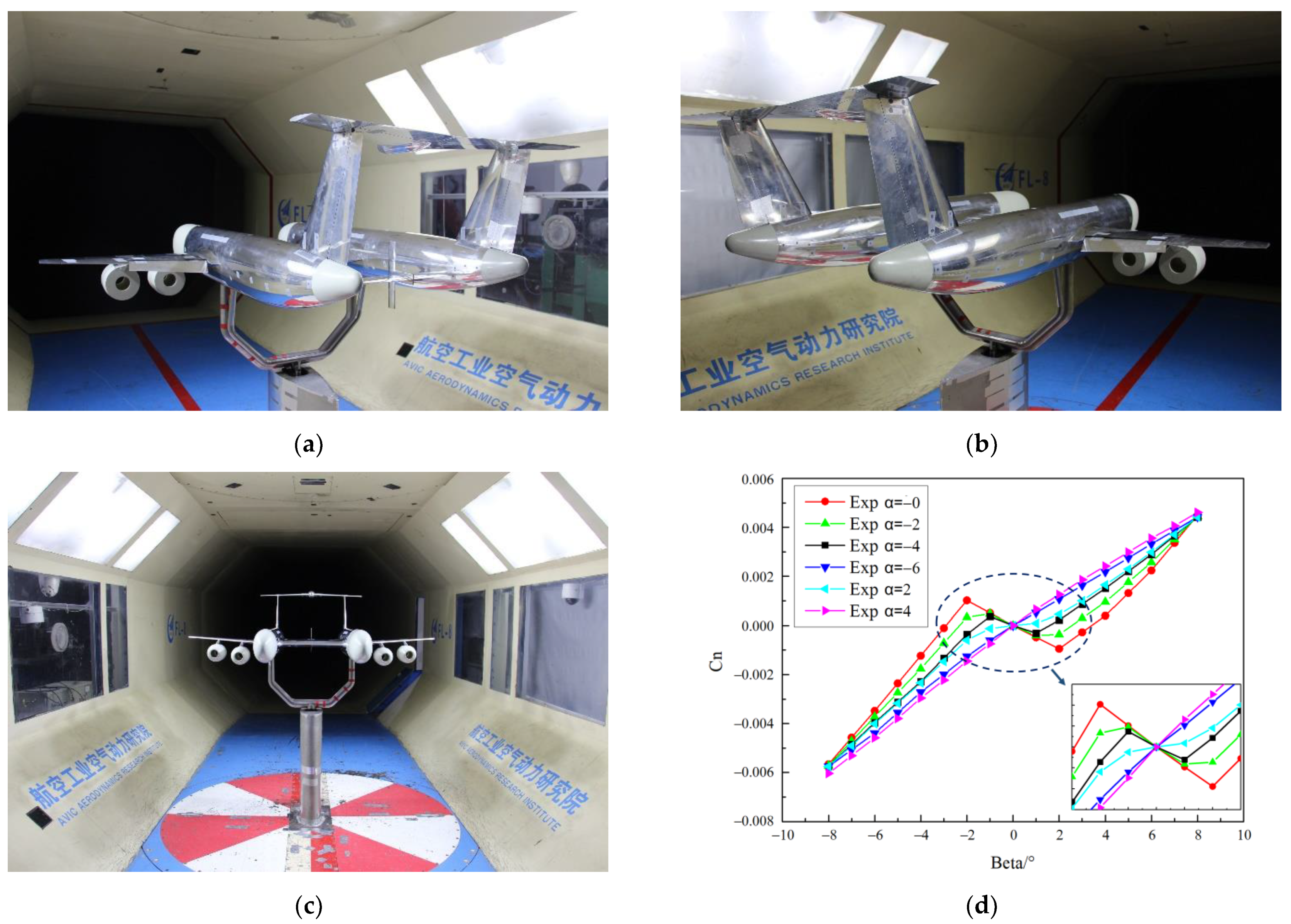
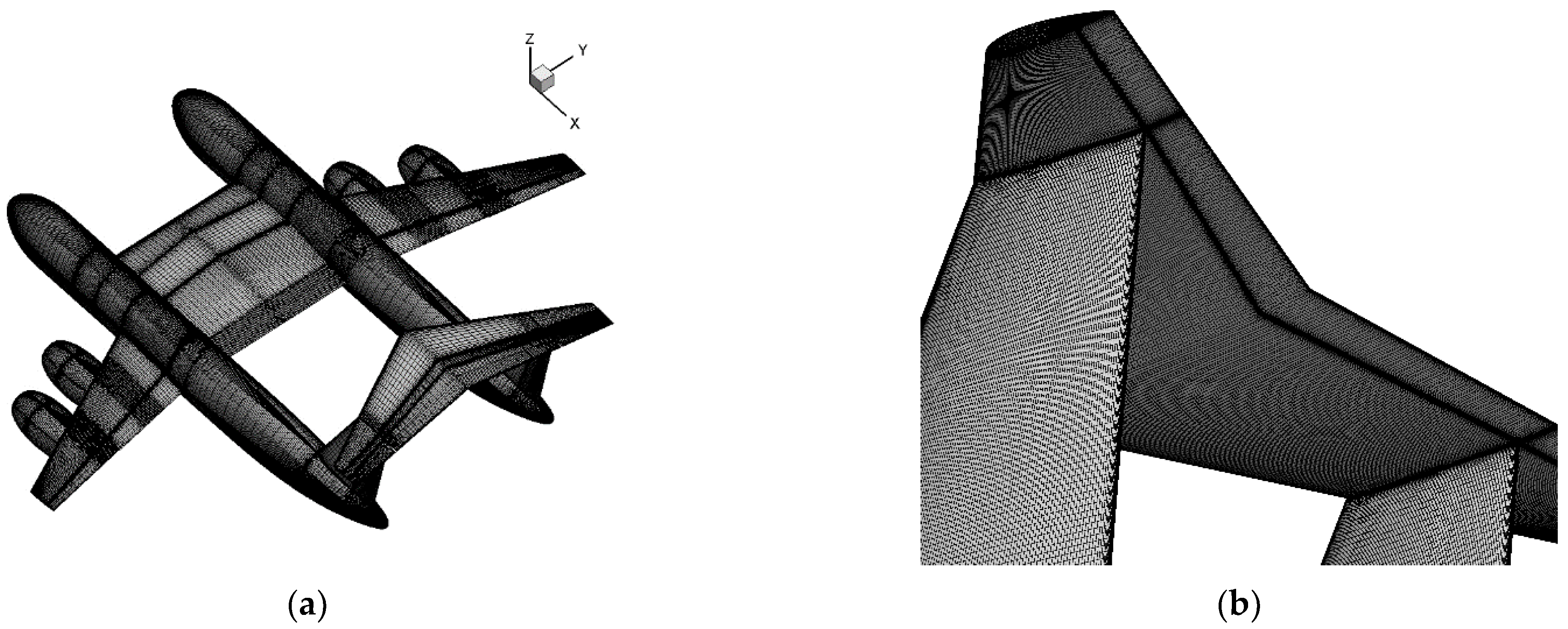
A demonstration aircraft with two airframes was designed for the purpose of performing better flying tests of newly design airfoils in the future, other than using a wing glove. To fully observe the test wing with these two airframes, the horizontal tail was designed to be thicker than usual, to place a special device. The wind tunnel experimental model is shown in Figure 8. Low-speed tests were carried out in the FL-8 wind tunnel of the Aviation Industry Corporation of China (AVIC), in which a 1:3.25 scale model was used, the test Reynolds number was ca. 1.5 × 10⁶ and the Mach number was 0.2. In these low-speed tests, an abdominally supported balance was used for force measurements, and the influence of its aerodynamic shape on the aircraft flow field and aerodynamic forces was subtracted by means of symmetrical balance measurement tests, as shown in Figure 8a–c.

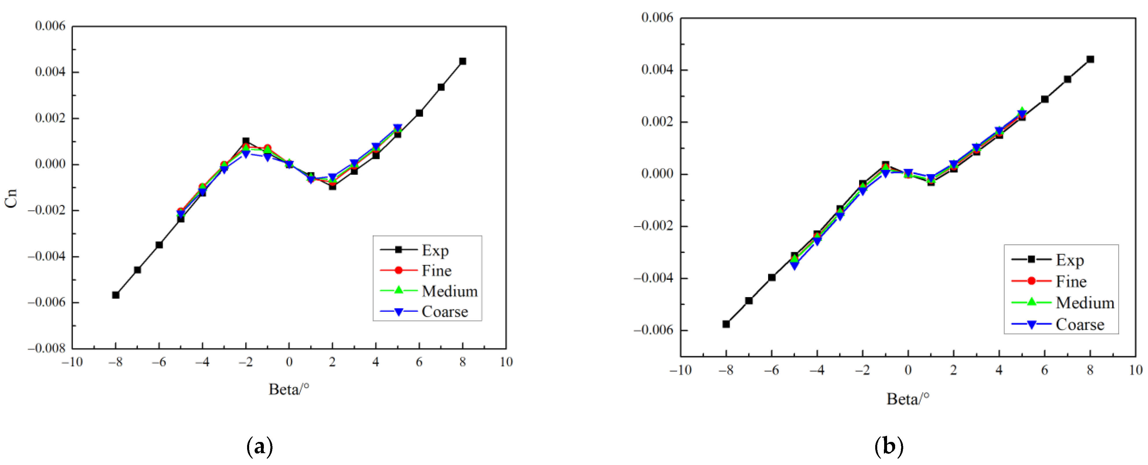
From the experimental data shown in Figure 8d, it can be seen that the aircraft lost SDS under a small angle of attack of between −4° and 0° and a small sideslip angle of between −4° and 4°. By contrast, under a large sideslip angle or positive angle of attack, the aircraft had SDS; even at an angle of attack of 2°, it could basically maintain SDS, and it only lost SDS at a sideslip angle of between −2° and 2°, unlike the larger range of sideslip angles in the previous case.

The main components of the aircraft that provide SDS are the vertical parts of its tail, and based on the experimental data, we speculated that the loss of SDS may have been due to one or more flow separations in the junctions of the horizontal and vertical tail parts, resulting in the vertical tail parts failing to provide SDS. When the aircraft has a small sideslip angle, the yaw moment generated by the vertical tail parts is small, as is that generated by the separation flow in the junctions of the horizontal and vertical tail parts, so the demonstration aircraft loses SDS under a small sideslip angle. Under a large sideslip angle, the yaw moment generated by the vertical tail parts is large, and even if corner separation flows are generated between the horizontal and vertical tail parts, they do not substantially affect the SDS. In addition, for this T-tail aircraft, the horizontal tail part is much thicker than usual, so the junction regions may suffer strong separation under a negative angle of attack, whereas under a positive angle of attack the separation in the junctions may be eased or even eliminated by the incoming flow, thereby allowing the aircraft to maintain SDS. Therefore, the demonstration aircraft was characterized by SDS under a large sideslip angle, which may be why it lacked SDS under a small sideslip angle.

3.2. Computational Grid and Verification

To verify the above preliminary analysis, we subjected the experimental model to CFD analysis. We assessed whether the calculation method and the grid used in the calculations met the accuracy requirements for subsequently analyzing the loss of SDS of the demonstration aircraft, then we analyzed its flow details in the T-tail junction regions and obtained data to support the subsequently improved design scheme.

To analyze the level of grid dependence, we used three different O-grids, with ca. 30, 50, and 70 million nodes, i.e., coarse, medium, and fine grids, respectively, which satisfied the criterion of y+ ≤ 1. Figure 9a shows the aircraft surface meshed with the coarse grid, and Figure 9b shows the surfaces of the horizontal and vertical tail parts meshed with the fine grid.

Table 2. Grid sizes.

Level	Grid	Horizontal Tail	Vertical Tail	Normal	Total Number of Nodes at the Tail Region
1	Coarse	181 × 201	161 × 201	29	2.12 × 106
2	Medium	257 × 285	229 × 285	41	6.01 × 106
3	Fine	365 × 401	325 × 401	57	17.27 × 106

shows the grids of the tail parts in detail, the distribution details of the horizontal and vertical tail parts are denoted “spanwise × chordwise” in Table 2.

The inlet and outlet boundary of the computation domain was 30 times the length of the span-wise in three directions (as the length of the span-wise is larger than the fuselage) and the aircraft was at the center of the domain, while the numerical set up was the same as mentioned above in Section 2.2. In the calculations, the Mach number was 0.2 and the Reynolds number was 1.5 × 10⁶, which is consistent with the experimental values. We calculated and verified the yaw moment of the whole aircraft at an angle of attack of between 0° and −4°.

Figure 10 compares the yaw moment coefficients between the experimental measurements and the SLA-IDDES calculations with the three different grids. As can be seen, the numerical results obtained with the medium and fine grids agree well with the experimental results; they capture well the loss of SDS of the aircraft under a small angle of attack and small sideslip angle, indicating that the calculation method with the medium or fine grid is suitable for capturing the overall macroscopic quantities of the demonstration aircraft. However, although the medium grid could capture the loss of SDS of the aircraft under a small sideslip angle, to analyze the flow separation in the T-tail junction regions in detail, the following results were all calculated using the fine grid.

3.3. Discussion

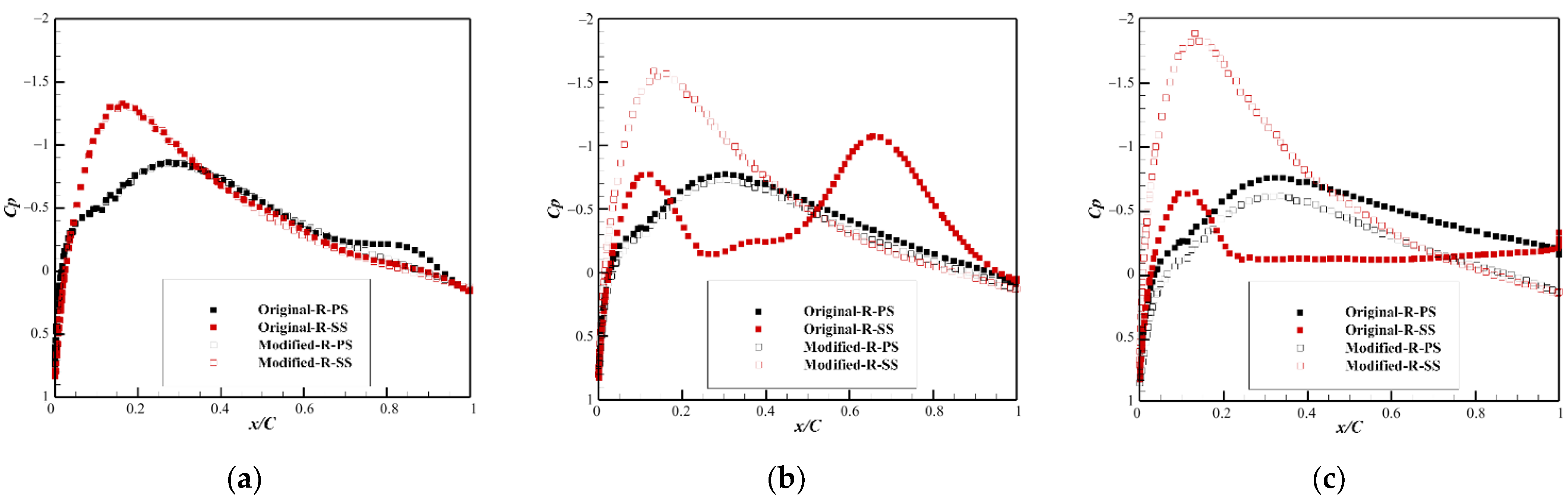
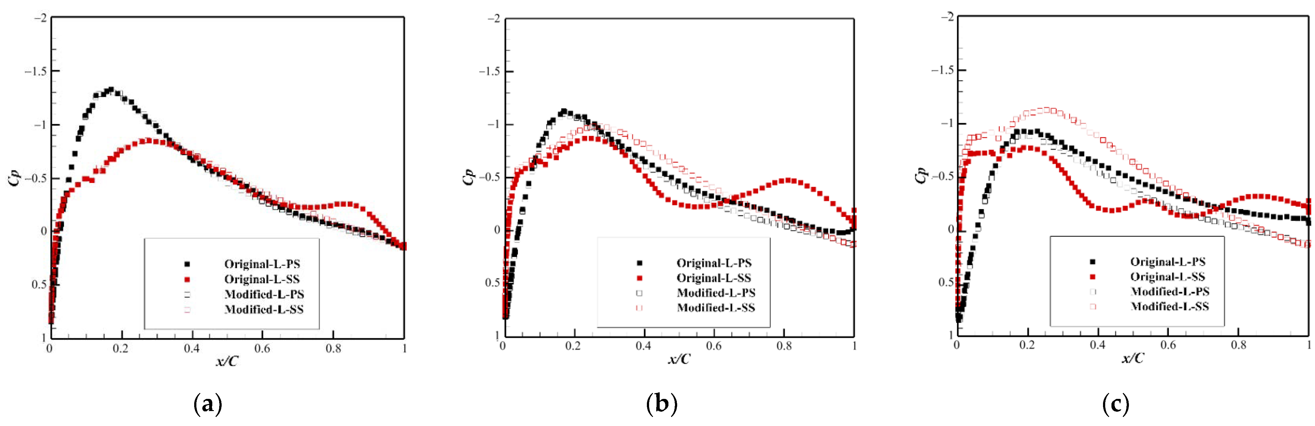
As discussed in Section 3.2, the experimental model of the demonstration aircraft was subjected to CFD analysis, the results were compared with the experimental measurements, and SLA-IDDES was shown to capture the loss of SDS under a small sideslip angle. To verify whether the conjecture made in Section 3.1 is correct, we must analyze the streamlines and C_p on the vertical tail surfaces.

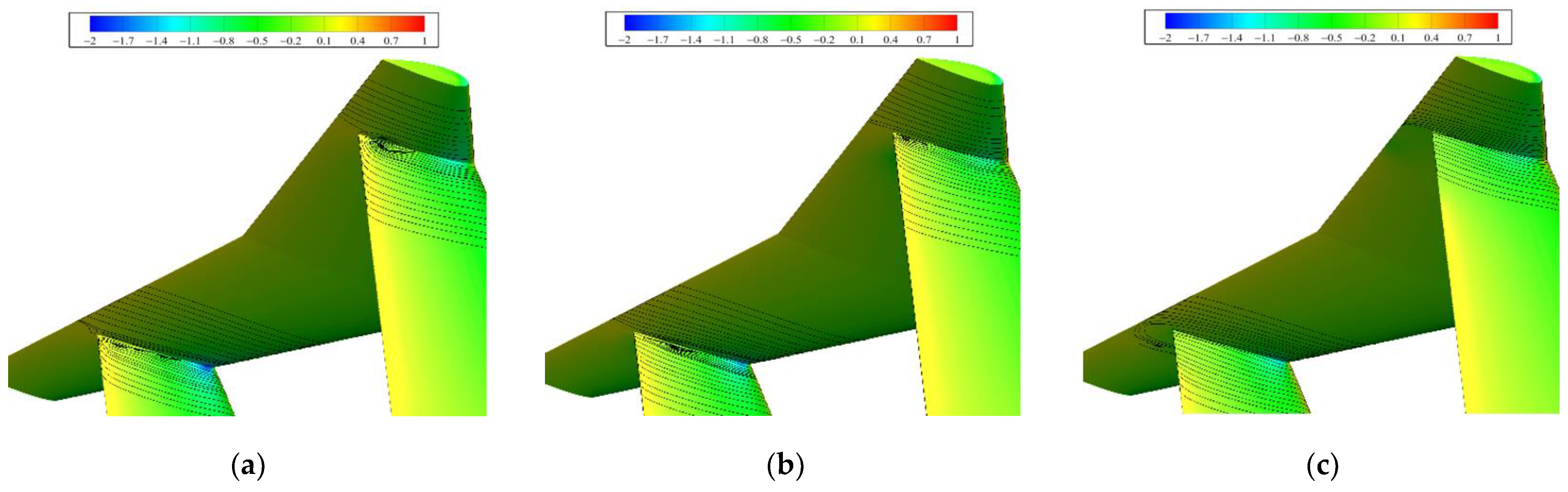
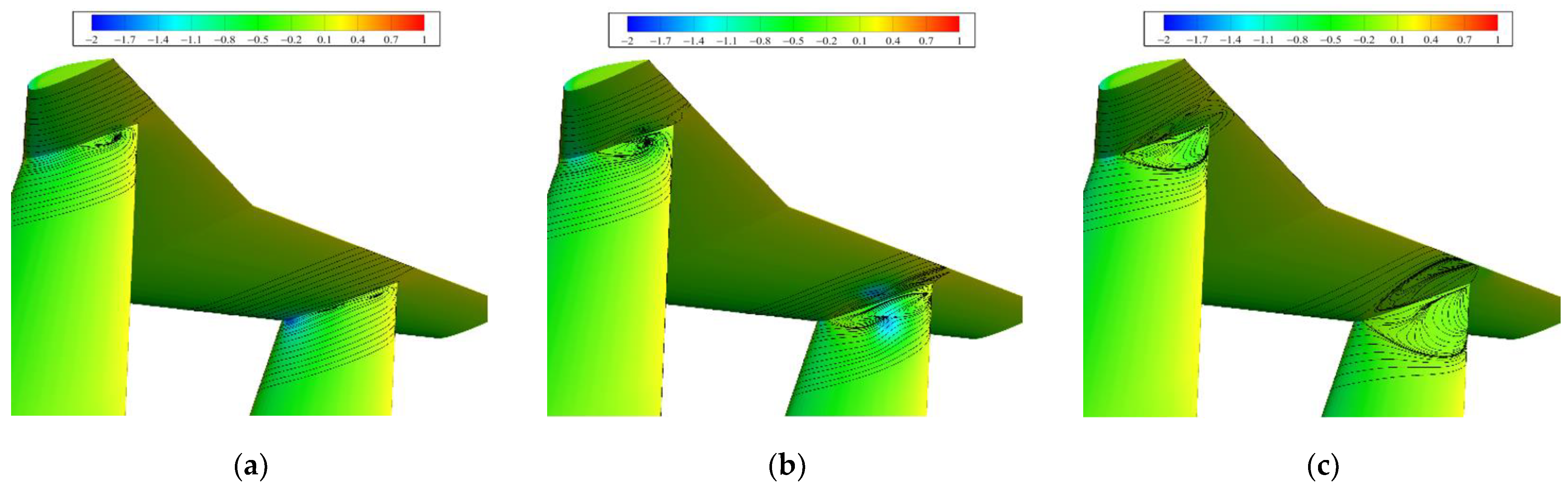
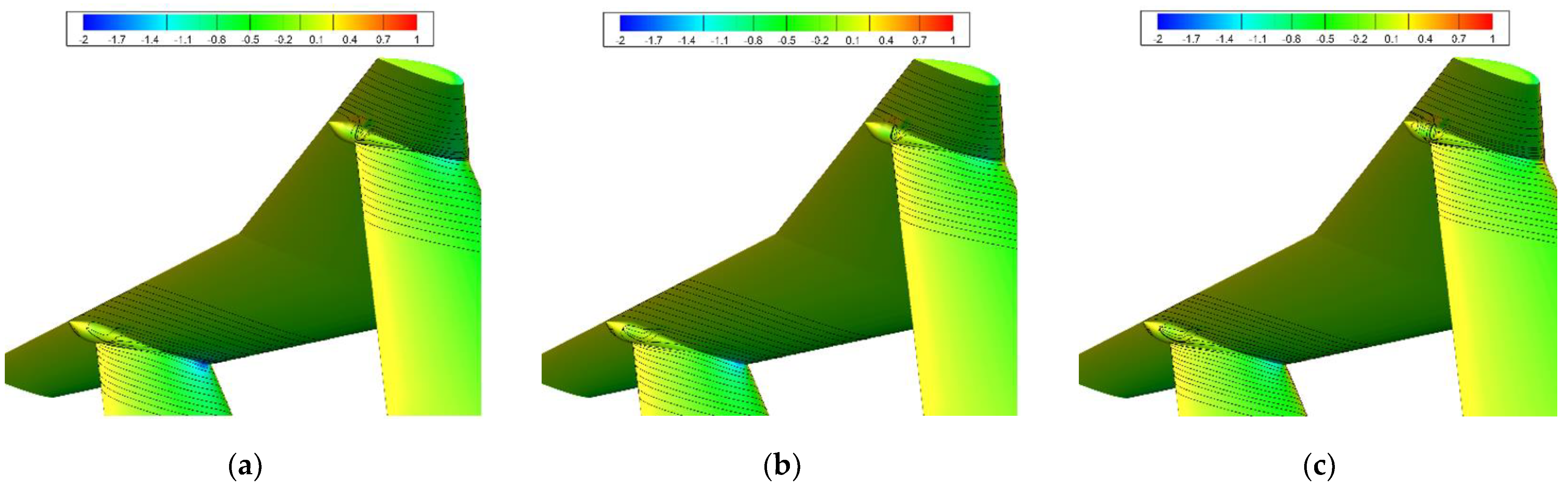
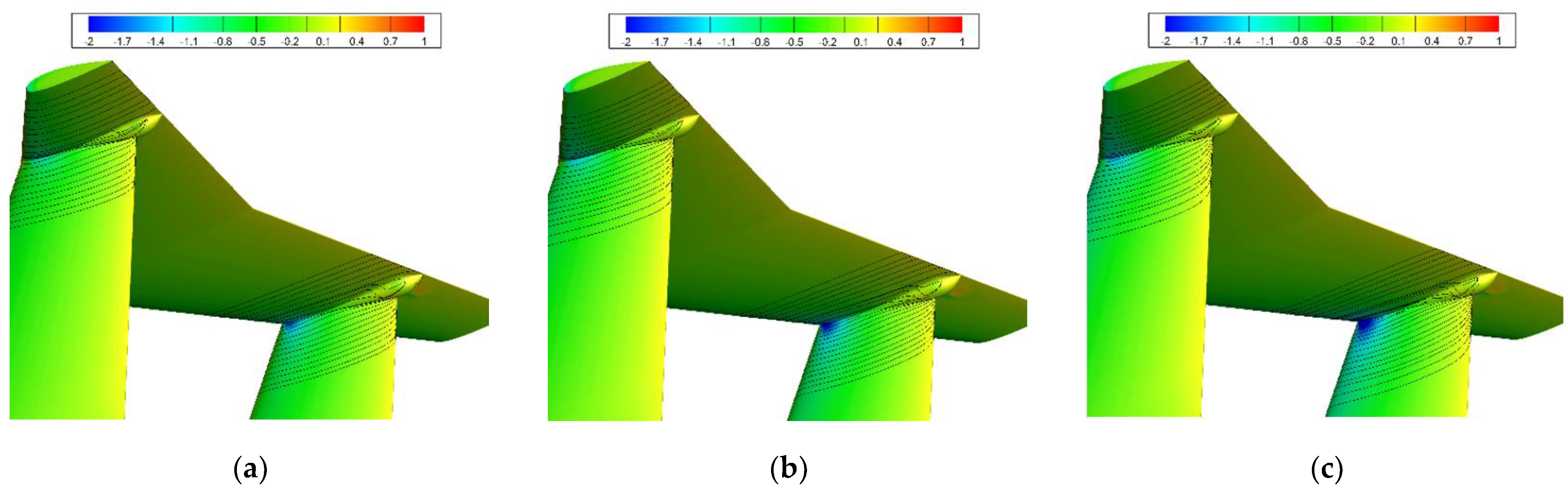
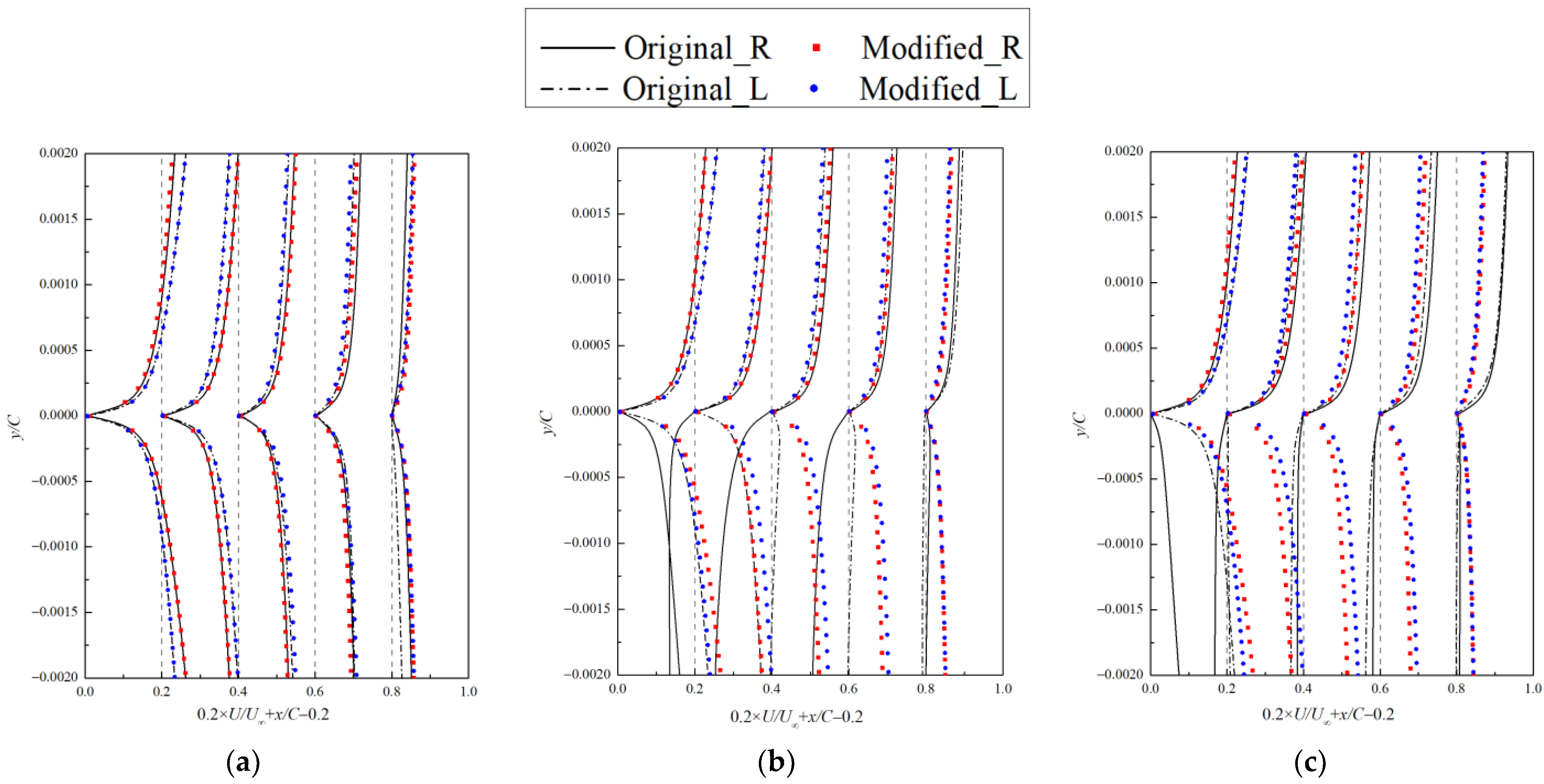
Figure 11 and Figure 12 show the surface streamlines at the pressure and suction sides, respectively, of the vertical tail parts of the demonstration aircraft at an angle of attack of 0° and a sideslip angle of 0°, 2°, and 4°. The streamlines show that there is separation on both the pressure and suction sides of the junction region at a sideslip angle of 0° and 2°, whereas at a sideslip angle of 4° the separation exists only on the suction side. Comparing Figure 11 and Figure 12 shows that the separation region on the suction side grows with an increasing sideslip angle, whereas that on the pressure side shrinks with an increasing sideslip angle. When the sideslip angle exceeds 4°, the separation region disappears and the aircraft has SDS, so the loss of SDS may be due to the separation on the suction side.

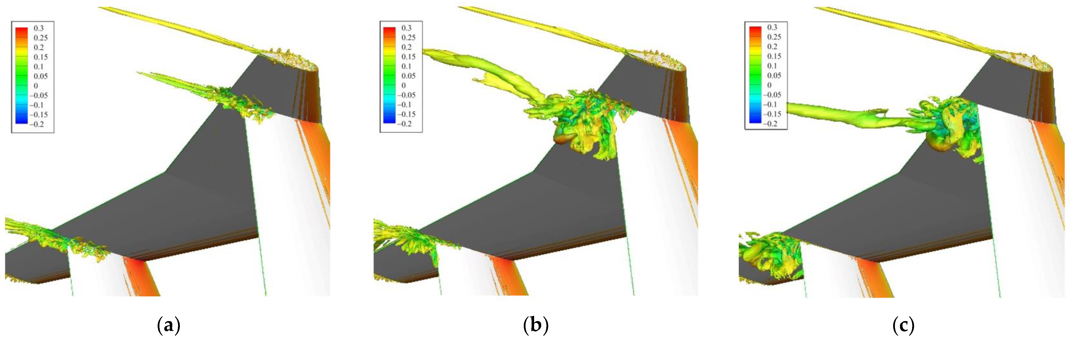
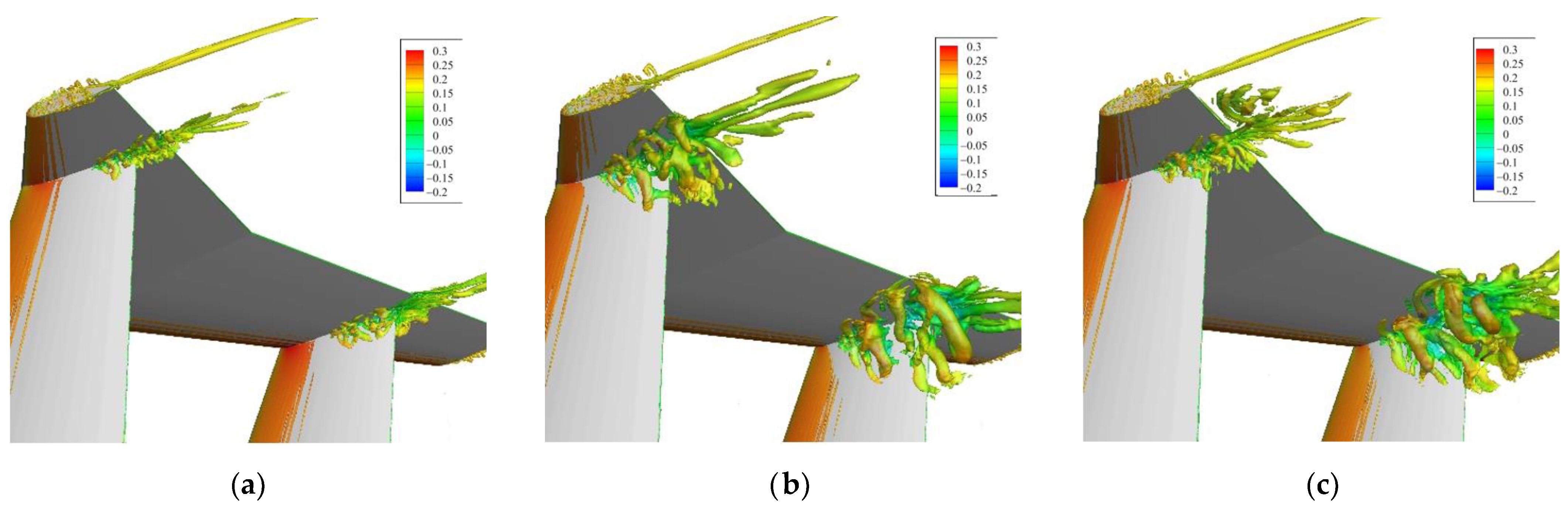
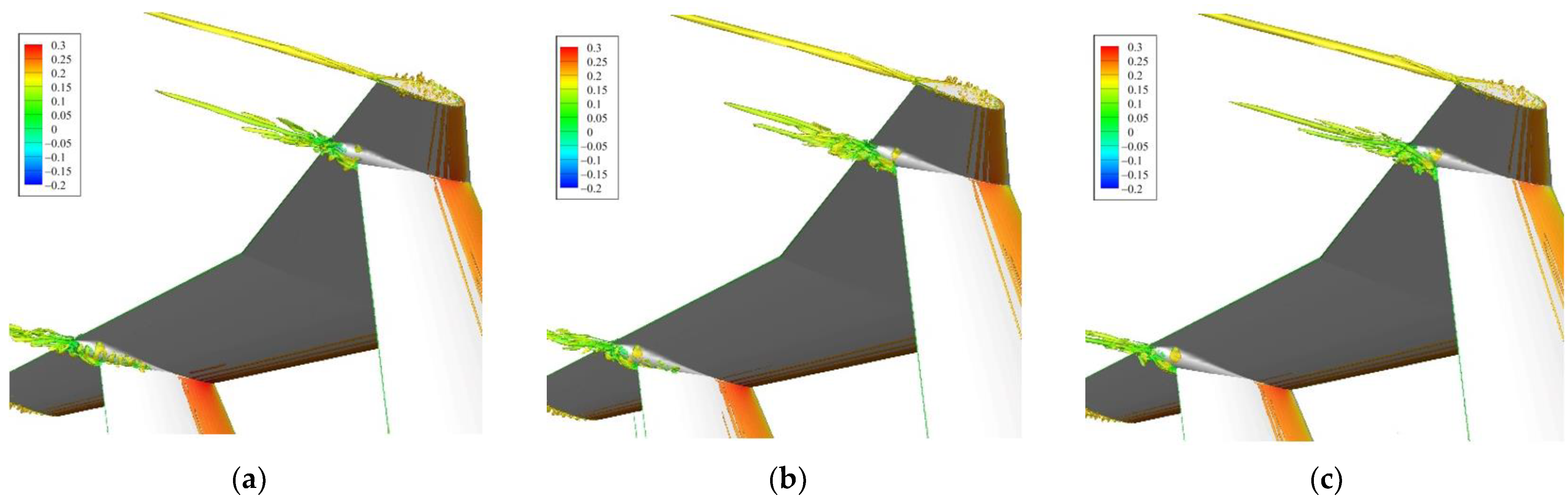
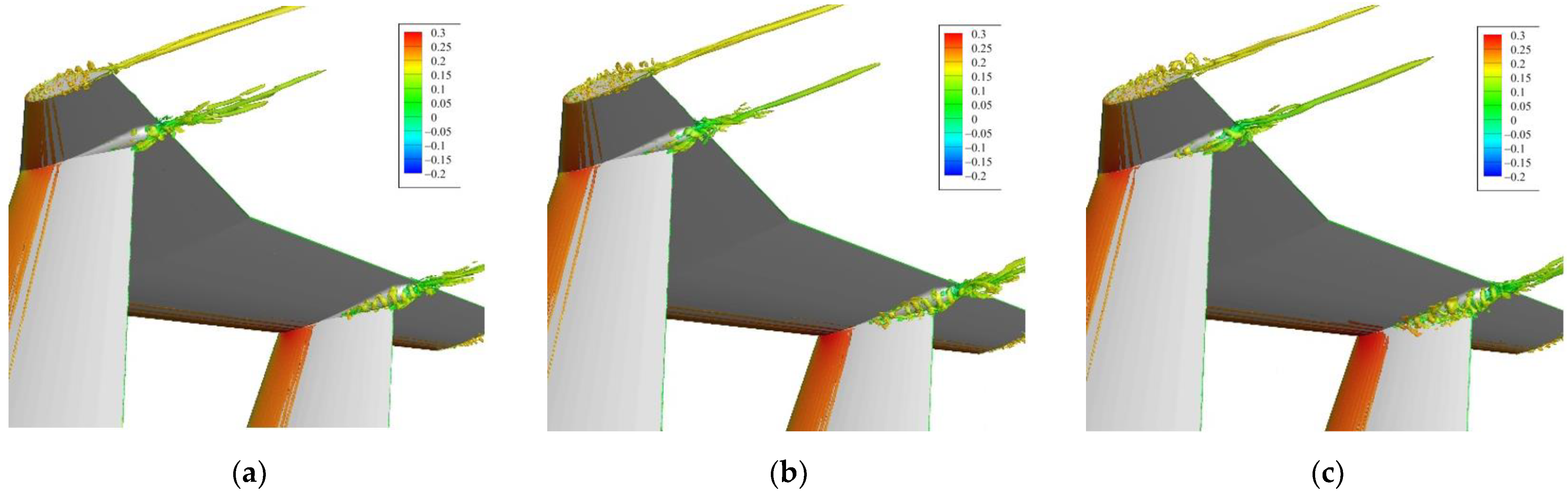
To see clearly the flow separation in the junction regions, we use an Ω isosurface [32] to analyze the flow detail. Figure 13 and Figure 14 show the Ω = 0.52 isosurface colored by the streamwise velocity normalized by the incoming velocity. Clearly, the separation regions on the suction side grow with an increasing sideslip angle. Separation begins after the point of maximum thickness of the local airfoil used for the vertical and horizontal tail parts; with an increasing sideslip angle, the separation start point moves upstream and the separation region grows sharply; and when the sideslip angle exceeds 2°, the separation shows a strong vortex–structure flow in the wake and even comes into contact with the horizontal tail part. Meanwhile, the separation vortices on the pressure side are limited in the junction regions by the incoming flow and have a limited effect on the vertical and horizontal tail parts, and with an increasing sideslip angle the separation is eliminated.

The question remains as to whether the main reason for the failure of the vertical tail parts is the separation on the pressure side, and this requires deep analysis. As the separated flow on the pressure side is smaller in extent and is restrained more easily than that on the suction side, flow-control measures to either weaken or eliminate the separated flow on the pressure side are taken, to control the flow in the horizontal-vertical tail junction areas, which is more conducive to analyzing the specific causes of the loss of SDS.

In addition, with the separation in the T-tail junction regions, not only will the aircraft suffer from extra drag (known as interference drag) and loss of SDS under a small sideslip angle, but the rudders at the trailing edges of the vertical tail parts may suffer from reduced efficiency at a small sideslip angle. Therefore, the separation in the junction regions must be weakened or better eliminated to improve the aircraft’s aerodynamic performance, and so flow control must be used in the junction regions.

4. Improved Design of T-Tail Junctions

4.1. Geometry

According to the literature [2,13,33], corner separation is mainly related to the BL, and with increasing thickness and energy of the BL, the corner separation becomes smaller or is even suppressed completely. However, because (i) there are no fairing cones in front of the horizontal-vertical tail junctions of the demonstration aircraft, and (ii) the leading edges of the horizontal and vertical tail parts almost coincide, the BLs here are thin and very likely to separate at the intersection regions. According to the rectification methods discussed by Simpson [1], the main fairing methods available for the T-tail junction regions of the demonstration aircraft are (i) chamfering for smooth transitions at the junction regions between the horizontal and vertical tail parts, (ii) leading-edge strakes, and (iii) fairing cones. However, using chamfering or leading-edge strakes would change the vertical tail configuration of the demonstration aircraft greatly, and as noted by Simpson [1], neither method is particularly effective at a large angle of attack or sideslip. Therefore, for the T-tail of this aircraft, the fairing-cone method is more suitable for increasing the thickness and energy of the BLs at the intersection regions of the T-tail on both sides, so as to reduce the separation size in the junction areas. This flow-control measure may not eliminate the separation on both sides, but it should do so on the pressure side of the vertical tail parts, and it could facilitate analyzing the loss of SDS of the demonstration aircraft and even relieve that problem.

To reduce the interference drag, while not increasing the frictional drag and pressure drag too much, we chose to use a small fairing cone instead of a whole one from the leading edge to the trailing edge of the junction region, such as the bullet fairing cone used on an IL-76 aircraft, as shown in Figure 15a. Here, the fairing cone is a simple cylinder with an elliptical cone at its rear, as shown in Figure 15b. The length Δx of the cylindrical part is 55% of the local airfoil length of the vertical tail part, and it is placed starting from the 45% position of that local airfoil toward the trailing edge of the horizontal tail part; its radius is r = 0.4 T, where T is the maximum thickness of the local airfoil of the vertical tail part, and the center of the cylinder is set at the trailing edge of the top of the vertical tail part. The modified model was subjected to CFD analysis for an angle of attack of 0° and a sideslip angle of between −4° and 4°, at which value the demonstration aircraft suffered the greatest loss of SDS; the Mach and Reynolds numbers were the same as those in Section 3.

4.2. Results and Discussion

Figure 16 compares the coefficients of yaw moment (C_n) and drag (C_d) of the T-tail obtained with the original and fairing cone configurations. Figure 16a shows that having the fairing cone at the junction region eliminates the loss of SDS and instead maintains it for a sideslip angle between −4° and 4°; in which range, the original model showed a fairly serious loss of SDS. Figure 16b shows that the fairing cone obviously reduced the drag of the T-tail of the aircraft: at a sideslip angle of 0°, the drag was reduced by ca. 9% compared with that of the original T-tail, and with increasing sideslip angle, the drag reduction ratio of the modified model increased, reaching ca. 17% at a sideslip angle of 4°. Considering that the pressure side of the vertical tail parts of the original model had no clear separation, the fairing cone seems to reduce part of the separation on the suction side.

To assess further the effectiveness of the fairing cone, Figure 17 and Figure 18 show the streamlines and C_p distribution on the pressure and suction sides, respectively, of the vertical tail parts of the modified model. Compared with Figure 11 and Figure 12, it is clear that the separation on the pressure side is eliminated by having the fairing cone in the junction region, as it is on the suction side. On the suction side of the vertical tail parts, the original model shows fairly a large separation on, not only the vertical tail parts, but also the horizontal tail part, whereas the modified model shows no flow separation.

As in Section 3, we again use an Ω isosurface here to analyze the flow details, as shown in Figure 19 and Figure 20. Compared with Figure 13 and Figure 14, in the modified model, the separation exists only at the backs of the fairing cones on the pressure side of the vertical tail parts; on the suction side of the tail, although the flow seems less stable and there are some small vortex structures at the vertical tail part on the right (as seen from the tail of the aircraft), the vortex structures are limited to the fairing-cone regions and there is no separation on the vertical and horizontal tail parts.

To analyze the reason for the T-tail failure in the original model, Figure 21 and Figure 22 show the C_p distributions of the original and modified models at the junction region just under the fairing cone, and Figure 23 shows the u-wise velocity profile normalized with the freestream velocity at the same location, to clearly show the location of flow separation; in Figure 23, y/C is the location away from the airfoil surface, with a positive value meaning the pressure side of the airfoil, and a negative value meaning the suction side. In Figure 21, Figure 22 and Figure 23, R means the right vertical tail part (as seen from the tail of the aircraft), L means the left vertical tail part, SS means the suction side, and PS means the pressure side.

As shown in Figure 21 and Figure 22, it seems that, at a sideslip angle of 0°, the C_p distributions of the original and modified models are basically the same, as are the velocity profiles. This is the case, except at the trailing edge, where the pressure side of the right vertical tail part and the suction side of the left vertical tail part show some differences from the modified model, this being because the inner sides of the vertical tail parts endure more occlusion from the horizontal tail part, because the local airfoil is thicker than the outboard, thus the separation is triggered earlier at the trailing edge. Figure 21a, Figure 22a and Figure 23a do not show a clear separation, because the exact location is beneath the fairing cone; C_p and the velocity profile may be affected by the separation, but not right in the separation region.

At a sideslip angle of 2°, the C_p distributions on the pressure side of both the right and left vertical tail parts in the two models are also basically the same, but the C_p distribution on the suction side of the right and left vertical tail parts are rather different when comparing the original and modified models. The right vertical tail part of the original model shows two suction peaks, one at the leading edge and another at the trailing edge; and at x/C ≈ 0.2–0.5, C_p on the suction side is higher than that on the pressure side; meanwhile, the modified model shows only one suction peak at the leading edge. At the left vertical tail part, both the original and modified models show a low contribution to SDS at the junction region, and the original model even shows a contribution to the loss of SDS. Moreover, the velocity profile shows that on the suction side of the right and left vertical tail parts, flow separation exists and starts before x/C = 40% and 60%, respectively, and the C_p value at the suction side of both the right and left vertical tail part shows a chaotic distribution because of the separation existing.

At a sideslip angle of 4°, the C_p distribution shows that the right vertical tail part of the modified model exhibits strong suction at the leading edge, whereas the original model exhibits very low suction from the leading edge to the trailing edge, because of flow separation, as shown in Figure 23c; the left vertical tail part of the modified model also shows a small suction, but the original model does not. Therefore, the failure of the vertical tail parts is due to flow separation on the suction side weakening the suction peak and finally causing the aircraft to lose SDS.

In addition, comparing Figure 21 and Figure 22 with Figure 23 shows that the left vertical tail part exhibits a higher suction peak than that of the right vertical tail part on the pressure side, which could be because the local airfoil on the horizontal tail at the pressure side of the left vertical is thicker than at the pressure side of the right vertical, and the local flow is accelerated in the junction regions, so the pressure side on the left vertical tail part exhibits a higher suction peak than that on the right pressure side. Therefore, in the junction regions, the right vertical tail part contributes the most to the SDS, which can be seen from the fact that in Figure 19, even with the fairing cone, the left vertical tail part contributes very little to the SDS.

Moreover, from the velocity profiles in Figure 23b,c, on the pressure side of the vertical tail parts, the right one shows an obvious separation; however, the velocity profile for the left vertical tail part shows a stable separation vortex in the junction region at a sideslip angle of 2°, because the u-wise velocity in the near-wall region is basically zero from x/C = 60% to the trailing edge. In addition, at a sideslip angle of 4°, the stable separation vortex breaks up, and the separation region grows sharply.

5. Conclusions

In this study, numerical simulations of a Rood airfoil and the JFs of a specially designed T-tail aircraft under small sideslip and attack angles were conducted using SLA-IDDES. As a newly improved method, SLA-IDDES is able to provide richer a flow field details than can traditional RANS methods, especially for small separation flows. Therefore, IDDES can be used as a state-of-the-art CFD tool for investigating small-separation configurations with different geometric characteristics, to understand better the physics of the onset and effects of flow separation under a small sideslip angle.

To ascertain whether SLA-IDDES could capture the small separation caused by strongly anisotropic flow, a standard model of Rood-airfoil JF was first simulated. Then, because this captured the flow details well, we used this new improved method to simulate a specially designed T-tail aircraft, to find out why in wind tunnel tests it loses SDS only at small angles of attack and sideslip.

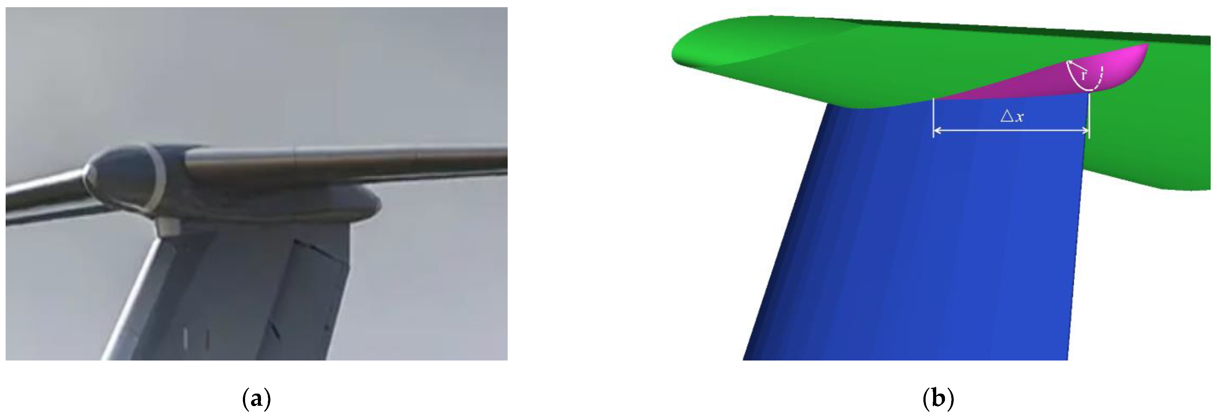
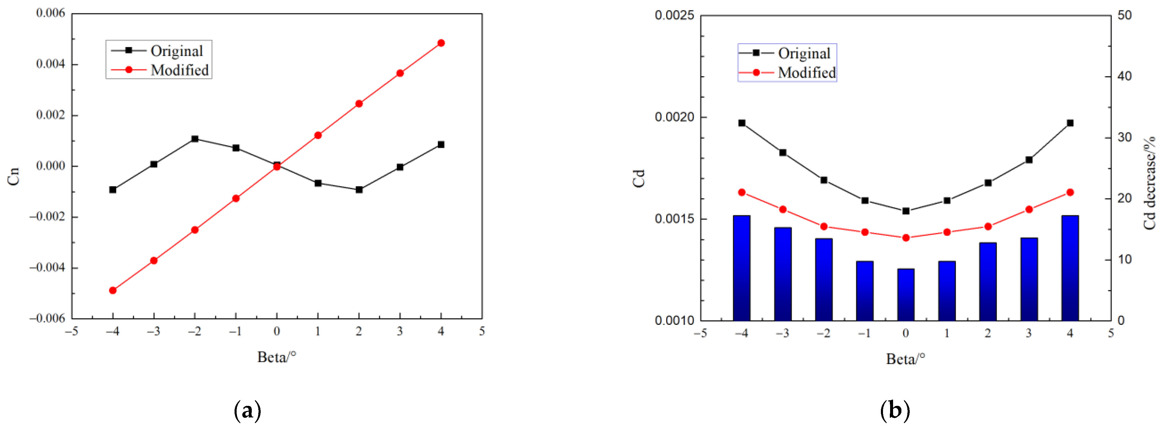
To verify the conjectured reason for the failure of the vertical tail parts, i.e., that the suction-side flow separation is the main reason why the aircraft loses SDS, we considered a small fairing cone (instead of a bullet one), to relieve or even eliminate the separation on the suction and pressure sides, the aim was to ascertain the reason for the loss of SDS and allow the aircraft to meet flight safety standards. From that research, we concluded that the onset and development of flow separation on the suction side of the vertical tail parts constitute the main reason for the loss of SDS, especially regarding the right (resp. left) vertical tail part under a positive (resp. negative) sideslip angle. Moreover, the qualitative analysis showed that fitting small fairing cones was sufficient for this T-tail aircraft to recover SDS, and doing so was effective for eliminating the loss of SDS and reducing the separation, so as to reduce the drag of the whole T-tail by at least 9%, including the interference drag and pressure drag. The specific conclusions of this study can be summarized as follows.

(1) SLA-IDDES captures macroscopic quantities fairly well, and although it is based on the k–ω SST RANS model, it avoids the inherent fault of the k-ω SST method (i.e., incorrectly predicting a four-vortex system) and captures sufficient flow details in the junction regions.

(2) Even with vertical tail parts that are quite large, the present T-tail aircraft loses SDS at a small sideslip angle when flow separation is triggered in the junction regions, this being because the vertical tail parts under that condition offer only very limited SDS from their other regions.

(3) Fitting small fairing cones relieves the flow separation in the junction regions; doing so completely eliminates the separation on the pressure side and limits that in the fairing-cone regions on the suction side. This avoids loss of SDS and rudder failure at a small sideslip angle, reduces the extra drag produced by flow separation, and allows the modified aircraft to retain SDS.

(4) The main reason for vertical-tail failure at a small sideslip angle is that the junction regions trigger separation flow on the suction side; this then reduces greatly the suction peak on the suction side, and a loss of SDS ensues when the vertical tail parts fail to provide sufficient SDS under this condition. Thus, the vertical tail parts fail at small sideslip angles.

Regarding future work, the present study considered only one type of fairing cone, and to extend the present results, it would be of interest to analyze and discuss the effects of fairing-cone radii, length, and location.

References

1. Simpson, R.L. Junction flows. Annu. Rev. Fluid Mech. 2001, 33, 415–443. [Google Scholar] [CrossRef]
2. Gand, F.; Deck, S.; Brunet, V.; Sagaut, P. Flow dynamics past a simplified wing body junction. Phys. Fluids 2010, 22, 115111. [Google Scholar] [CrossRef]
3. Paciorri, R.; Bonfiglioli, A.; Di Mascio, A.; Favini, B. RANS simulations of a junction flow. Int. J. Comput. Fluid Dyn. 2005, 19, 179–189. [Google Scholar] [CrossRef]
4. Devenport, W.J.; Simpson, R.L. Time-dependent and time-averaged turbulence structure near the nose of a wing-body junction. J. Fluid Mech. 1990, 210, 23–55. [Google Scholar] [CrossRef]
5. Simpson, R.L. Aspects of turbulent boundary-layer separation. Prog. Aerosp. Sci. 1996, 32, 457–521. [Google Scholar] [CrossRef]
6. Fleming, J.L.; Simpson, R.L.; Cowling, J.E.; Devenport, W.J. An experimental study of a turbulent wing-body junction and wake flow. Exp. Fluids 1993, 14, 366–378. [Google Scholar] [CrossRef]
7. Ölçmen, S.M.; Simpson, R.L. Influence of wing shapes on surface pressure fluctuations at wing-body junctions. AIAA J. 1994, 32, 6–15. [Google Scholar] [CrossRef]
8. Ölçmen, S.M.; Simpson, R. Theoretical and experimental pressure-strain comparison in a pressure-driven three-dimensional turbulent boundary layer. In Proceedings of the Theroretical Fluid Mechanics Conference, New Orleans, LA, USA, 17–20 June 1996; p. 2141. [Google Scholar]
9. Ölçmen, S.M.; Simpson, R.L. Experimental transport-rate budgets in complex 3-D turbulent flow near a wing/body junction. Int. J. Heat Fluid Flow 2008, 29, 874–890. [Google Scholar] [CrossRef]
10. Ozcan, O.; Ölçmen, S.M. Measurements of turbulent flow behind a wing-body junction. AIAA J. 1988, 26, 494–496. [Google Scholar] [CrossRef]
11. Anderson, S.D.; Eaton, J.K. Experimental study of a pressure-driven, three-dimensional, turbulent boundary layer. AIAA J. 1987, 25, 1086–1092. [Google Scholar] [CrossRef]
12. Gand, F.; Monnier, J.C.; Deluc, J.M.; Choffat, A. Experimental study of the corner flow separation on a simplified junction. AIAA J. 2015, 53, 2869–2877. [Google Scholar] [CrossRef]
13. Barber, T.J. An investigation of strut-wall intersection losses. J. Aircr. 1978, 15, 676–681. [Google Scholar] [CrossRef]
14. Wen, J.; Wang, Y.; Deng, X. An experimental investigation on static directional stability. Chin. J. Aeronaut. 2016, 29, 1527–1540. [Google Scholar] [CrossRef]
15. Gand, F.; Brunet, V.; Deck, S. Experimental and numerical investigation of a wing-body junction flow. AIAA J. 2012, 50, 2711–2719. [Google Scholar] [CrossRef]
16. Apsley, D.D.; Leschziner, M.A. Investigation of advanced turbulence models for the flow in a generic wing-body junction. Flow Turbul. Combust. 2001, 67, 25–55. [Google Scholar] [CrossRef]
17. Parneix, S.; Durbin, P.A.; Behnia, M. Computation of 3-D turbulent boundary layers using the V2F model. Flow Turbul. Combust. 1998, 60, 19–46. [Google Scholar] [CrossRef]
18. Lien, F.S.; Kalitzin, G.; Durbin, P.A. RANS modeling for compressible and transitional flows. In Proceedings of the Summer Program; Center for Turbulence Research, Stanford University: Stanford, CA, USA, 1998; Volume 1. [Google Scholar]
19. Eisfeld, B.; Rumsey, C.L.; Togiti, V.; Braun, S.; Stürmer, A. Reynolds-stress model computations of NASA juncture flow experiment. AIAA J. 2022, 60, 1643–1662. [Google Scholar] [CrossRef]
20. Kegerise, M.A.; Neuhart, D.; Hannon, J.; Rumsey, C.L. An experimental investigation of a wing-fuselage junction model in the NASA Langley 14-by 22-foot subsonic wind tunnel. In AIAA Scitech 2019 Forum; American Institute of Aeronautics and Astronautics: Reston, VA, USA, 2019; p. 77. [Google Scholar]
21. Rumsey, C.L. The NASA juncture flow test as a model for effective CFD/experimental collaboration. In Proceedings of the 2018 Applied Aerodynamics Conference, Atlanta, GA, USA, 25–29 June 2018; p. 3319. [Google Scholar]
22. Rumsey, C.L.; Neuhart, D.; Kegerise, M.A. The NASA juncture flow experiment: Goals, progress, and preliminary testing. In Proceedings of the 54th AIAA Aerospace Sciences Meeting, San Diego, CA, USA, 4–8 January 2016; p. 1557. [Google Scholar]
23. Rumsey, C.L.; Ahmad, N.N.; Carlson, J.R.; Kegerise, M.A.; Neuhart, D.; Hannon, J.; Jenkins, L.N.; Yao, C.-S.; Balakumar, P.; Gildersleeve, S.; et al. CFD comparisons with updated NASA juncture flow data. In AIAA Scitech 2021 Forum; American Institute of Aeronautics and Astronautics: Reston, VA, USA, 2021; p. 1427. [Google Scholar]
24. Shur, M.L.; Spalart, P.R.; Strelets, M.K.; Travin, A.K. A hybrid RANS–LES approach with delayed-DES and wall-modelled LES capabilities. Int. J. Heat Fluid Flow 2008, 29, 1638–1649. [Google Scholar] [CrossRef]
25. Shur, M.L.; Spalart, P.R.; Strelets, M.K.; Travin, A.K. An enhanced version of DES with rapid transition from RANS to LES in separated flows. Flow Turbul. Combust. 2015, 95, 709–737. [Google Scholar] [CrossRef]
26. Ölçmen, S.M.; Simpson, R.L. An experimental study of a three-dimensional pressure-driven turbulent boundary layer. J. Fluid Mech. 1995, 290, 225–262. [Google Scholar] [CrossRef] [Green Version]
27. Ryu, S.; Emory, M.; Iaccarino, G.; Campos, A.; Duraisamy, K. Large-eddy simulation of a wing–body junction flow. AIAA J. 2016, 54, 793–804. [Google Scholar] [CrossRef]
28. Paik, J.; Escauriaza, C.; Sotiropoulos, F. On the bimodal dynamics of the turbulent horseshoe vortex system in a wing-body junction. Phys. Fluids 2007, 19, 045107. [Google Scholar] [CrossRef]
29. Zhang, L.; Li, J.; Mou, Y.F.; Zhang, H.; Shi, W.B.; Jin, J. Numerical investigation of flow around a multi-element airfoil with hybrid RANS–LES approaches based on SST model. J. Mech. 2018, 34, 123–134. [Google Scholar] [CrossRef]
30. Lee, J.P.; Chen, J.H.; Hsin, C.Y. Study of junction flow structures with different turbulence models. J. Mar. Sci. Technol. 2017, 25, 178–185. [Google Scholar]
31. Alberts, J. Wall-Resolved Large Eddy Simulation of a Wing–Body Junction: High-Fidelity Data Generation for Data-Driven Turbulence Modelling. Master’s Thesis, Delft University of Technology, Delft, The Netherlands, 2021. [Google Scholar]
32. Liu, C.; Wang, Y.; Yang, Y.; Duan, Z. New omega vortex identification method. Sci. China Phys. Mech. Astron. 2016, 59, 684711. [Google Scholar] [CrossRef]
33. Gessner, F.B. The origin of secondary flow in turbulent flow along a corner. J. Fluid Mech. 1973, 58, 1–25. [Google Scholar] [CrossRef]
Figure 1. (a) Computational domain according to Ryu et al. [27]. (b) Near-wall region with fine grid.
Aerospace 09 00567 g001
Figure 2. Mean Cp calculated by SLA-IDDES: y/T = (a) 0.132 and (b) 1.726.
Aerospace 09 00567 g002
Figure 3. Mean velocity profile and Reynold stress in the leading edge region calculated using three different methods: (a) velocity profile and (b) Reynold stress.
Aerospace 09 00567 g003
Figure 4. Streamlines at junction nose calculated using kω SST: (a) streamlines; (b) four-vortex system.
Aerospace 09 00567 g004
Figure 5. Streamlines at junction nose calculated using SLA-IDDES: (a) streamlines; (b) two-vortex system.
Aerospace 09 00567 g005
Figure 6. Secondary and tertiary separation lines on the bottom wall: (a) RANS/LES [27]; (b) wall-resolved LES [31]; (c) SLA-IDDES.
Aerospace 09 00567 g006
Figure 7. Streamlines on bottom wall calculated using SLA-IDDES: (a) streamlines with a fishtail shape at trailing edge; (b) flow separation at the trailing edge, colored by the streamwise velocity.
Aerospace 09 00567 g007
Figure 8. Experimental model of the demonstration aircraft in a wind tunnel: (a) left side of the aircraft; (b) right side of the aircraft; (c) front of the aircraft; (d) results for coefficient of yaw moment.
Aerospace 09 00567 g008
Figure 9. (a) Surface mesh of whole demonstration aircraft with a coarse gird. (b) Surface mesh of the T-tail with a fine grid.
Aerospace 09 00567 g009
Figure 10. Coefficient of yaw moment calculated with three different grids, and comparison with the experimental results. (a) α = 0° (b) = −4°.
Aerospace 09 00567 g010
Figure 11. Streamlines and Cp distribution on the pressure side of the vertical tail parts: β = (a) 0°, (b) 2°, and (c) 4°.
Aerospace 09 00567 g011
Figure 12. Streamlines and Cp distribution on the suction side of the vertical tail parts: β = (a) 0°, (b) 2°, and (c) 4°.
Aerospace 09 00567 g012
Figure 13. Ω = 0.52 isosurface, looking from the pressure side of vertical tail parts: β = (a) 0°, (b) 2°, and (c) 4°.
Aerospace 09 00567 g013
Figure 14. Ω = 0.52 isosurface, looking from the suction side of vertical tail parts: β = (a) 0°, (b) 2°, and (c) 4°.
Aerospace 09 00567 g014
Figure 15. Two different fairing-cone models: (a) bullet fairing cone; (b) schematic of the fairing cone model used herein.
Aerospace 09 00567 g015
Figure 16. Coefficients of (a) yaw moment and (b) drag calculated with original (black) and modified (red) model.
Aerospace 09 00567 g016
Figure 17. Streamlines and Cp distribution on pressure side for modified model: β = (a) 0°, (b) 2°, and (c) 4°.
Aerospace 09 00567 g017
Figure 18. Streamlines and Cp distribution on the suction side for the modified model: β = (a) 0°, (b) 2°, and (c) 4°.
Aerospace 09 00567 g018
Figure 19. Ω = 0.52 isosurface, looking from the pressure side of modified model: β = (a) 0°, (b) 2°, and (c) 4°.
Aerospace 09 00567 g019
Figure 20. Ω = 0.52 isosurface, looking from the suction side of modified model: β = (a) 0°, (b) 2°, and (c) 4°.
Aerospace 09 00567 g020
Figure 21. Cp distributions on right vertical tail part of the original and modified models: β = (a) 0°, (b) 2°, and (c) 4°.
Aerospace 09 00567 g021
Figure 22. Cp distributions on the left vertical tail part of the original and modified models: β = (a) 0°, (b) 2°, and (c) 4°.
Aerospace 09 00567 g022
Figure 23. u-wise velocity profiles in the near-wall region: β = (a) 0°, (b) 2°, and (c) 4°.
Aerospace 09 00567 g023