Mean Value-Based Parallel Collaborative Optimization Method for Modular Aircraft Structural Layout

Abstract

The conventional structural layout optimization method is usually used to solve the layout optimization problem of a single structure, but it is difficult to apply to the layout optimization problem of the modular aircraft structure containing multiple substructures. Therefore, this paper proposes the mean value-based parallel collaborative optimization method (MVPM) for modular aircraft structural layout. This method is a two-stage optimization method based on decomposition. The basic idea of the MVPM is decomposing the layout optimization problem of the modular aircraft structure into a system coordination problem and several independent subsystem optimization problems by introducing coordination variables. The subsystem optimizes each aircraft structure. Under the constraints of the structure itself, the performance of each structure is better, and the shared variables are as close to the coordination variables as possible. The system coordination adjusts the coordination variables according to the optimization results of each subsystem. With constant iteration between the system and subsystems, the shared variables of each subsystem eventually agree with the coordination variables. The numerical test results show that the MVPM has high optimization efficiency and stability.

1. Introduction

With the development of the global market economy, increasing competition in various fields and diversification of customer demand for product functions, the conflict between product diversity, product development and production costs has become more obvious. Modular design strategy is to design different types of products at the same time on a product platform. While meeting the customer’s needs for product functional diversity, it shortens the product development and reduces the product cost; therefore, modular design strategy has received extensive attention on both industrial applications [1] and academic research [2].

Modular aircraft refers to a series of aircraft formed by dividing and organizing various modules of the aircraft by using modular ideas. These aircraft are composed of a series of general modules and dedicated modules. Their general modules may be the wings, fuselage sections or engines of the aircraft and may also be some equipment or some systems [3]. These general modules constitute a general platform for modular aircraft [4]. Based on the general platform, different types of aircraft are formed by adding or changing different dedicated modules to accomplish different mission requirements. Dedicated modules are unique to each aircraft, and dedicated modules are the source of differentiation of functions and features of different types of aircraft. Simpson et al. [5,6] and Jiao et al. [7] gave a detailed summary of the research and applications related to product families, respectively.

Compared with the traditional single-type aircraft design, the modular aircraft design strategy is to develop multiple types of aircraft on the general platform at the same time, which can greatly reduce the cost of aircraft design and manufacturing and shorten the aircraft design cycle. The general platform facilitates the expansion of the aircraft family, and it is easy to add a new member to meet the newly increased demand, while helping reduce maintenance and operating costs [8]. The modular design strategy also has some shortcomings and risks [9]. The general platform enables generality between different aircraft but also makes each aircraft pay a certain performance price [10]. Compared with the design of a single type aircraft, the development cost and development difficulty of a modular aircraft are much higher [11], and once a problem occurs on the general platform, the scope of influence will expand to all aircrafts.

The purpose of structural layout optimization of modular aircraft is to optimize the structural layout of general and dedicated modules with the help of an optimization algorithm so that the overall performance of the modular structure can be optimized. Layout optimization is a higher-level structural optimization problem, which is a comprehensive optimization problem that includes topology, shape and size optimization. Structural layout optimization needs to determine the number, location, cross-sectional shape and size of each component of the structure. At present, the solution strategies for structural layout optimization problems can be roughly divided into three types: hybrid optimization [12,13,14], hierarchical optimization [15,16,17] and block optimization [18]. These three types of optimization strategies are usually used to solve the layout optimization problem of a single structure. The layout optimization of the modular structure is to optimize the layout of a series of related substructures at the same time. These substructures have exactly the same general modules and different dedicated modules, and the structural layout of each module affects each other. Therefore, the layout optimization of modular structure is a process of multistructure layout coordination, which is difficult to solve with conventional structural layout optimization strategies. In addition, the performance of a modular structure must be compromised compared to the performance of each structure designed individually. The general platform makes each structure have a certain degree of generality, and the quality of the general platform determines the performance of the modular structure. Therefore, it can also be said that the layout optimization of the modular structure is a trade-off between the performance and the degree of generality [19].

In order to better solve the layout design problem of modular aircraft structure, this paper proposes a mean value-based parallel collaborative optimization method (MVPM). This method is a two-stage optimization method based on decomposition. The basic idea of the MVPM is decomposing the layout optimization problem of the modular aircraft structure into a system coordination problem and several independent subsystem optimization problems by introducing coordination variables. The system adjusts the coordination variables according to the feedback of each subsystem. Each subsystem is responsible for evaluating the coordination variables and feeding back the evaluation results to the system as the basis for adjusting the coordination variables. The process iterates between the system and each subsystem until the optimal solution is found.

The content of this paper is arranged as follows: The next section presents the modular structure layout optimization problem. Section 3 presents the mathematical expression of the modular structure layout design problem. Section 4 presents the MVPM in detail. Section 5 tests the MVPM with a typical nonconvex numerical example. Section 6 applies the MVPM to the wing structure layout design of a modular aircraft. Section 7 concludes this paper.

2. Problem Description

Modular aircraft usually consist of a variety of aircraft for different purposes, such as the MQ-X UAV and “Poseidon”. The wing of the MQ-X UAV is divided into two sections: the inner wing is a general module, and the outer wings are dedicated modules. The span of the wing can be changed by replacing the dedicated module. The fuselage of the “Poseidon” is divided into front, middle and rear sections. The front section and the rear section of the fuselage are general modules, and the middle section of the fuselage is a dedicated module. The Poseidon aircraft can complete more than five different tasks by replacing different middle fuselages. Whether it is a modular wing structure or a modular fuselage structure, it consists of a series of general modules and dedicated modules, and the general modules are identical in different aircraft types. The layout optimization of the modular structure is to optimize the structural layout of each general module and dedicated module at the same time. The key is to comprehensively consider the requirements of all substructures and design the structural layout of general modules suitable for all substructures.

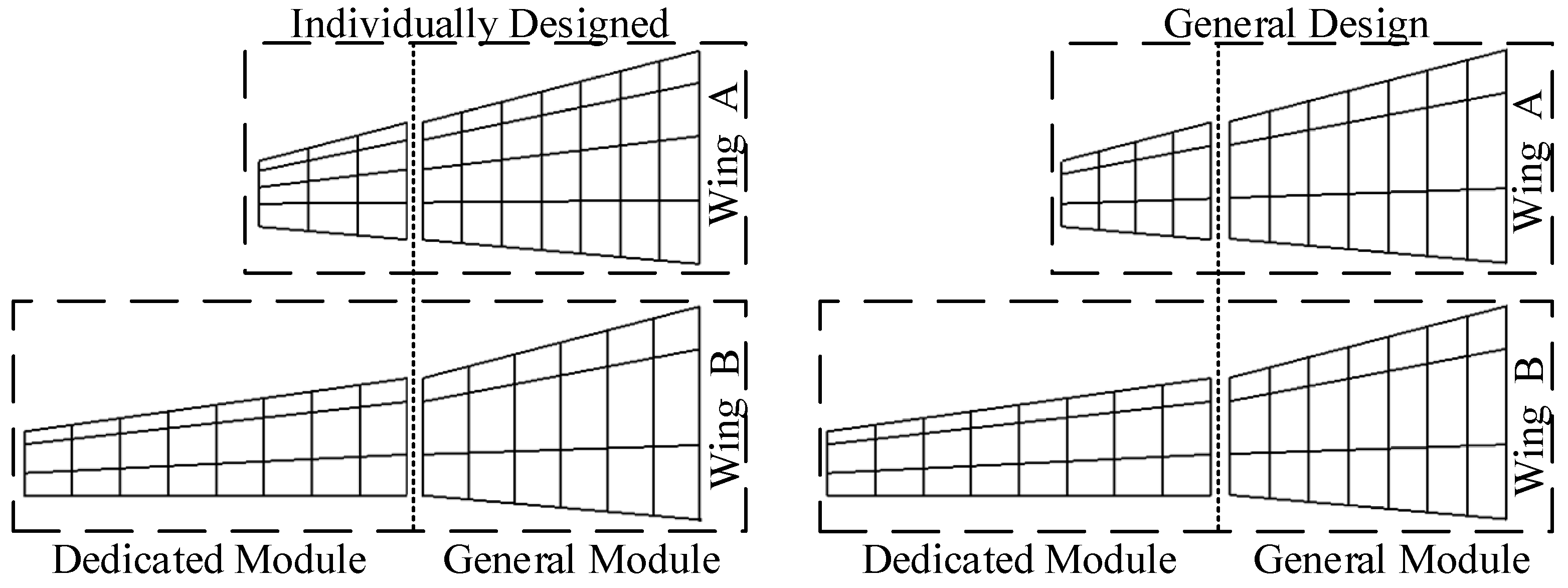
When generality is not considered, the optimal structural layout of generalized modules in different substructures is usually different. As shown in Figure 1, the modular wing structure has a general module inside and a dedicated module outside. The optimal structural layout of general modules is different when matched with different dedicated modules. When the general design is adopted, the general module adopts the exact same design in different wings, and due to the change of the general module structure layout, the structure layout of each special module has also changed accordingly. Therefore, the layout optimization of the modular structure should be designed simultaneously for all modules and take into account the mutual influence of each module.

3. Mathematical Model

The conventional structural layout optimization problem is to optimize the layout of a single structure, and its mathematical description is as follows:

$$\begin{array}{c}\mathrm{find}\\ \min \\ \mathrm{s}.\mathrm{t}.\end{array}\begin{array}{c}\\ \\ \end{array}\begin{array}{l}\mathit{x}\hfill \\ f(\mathit{x})\hfill \\ \mathit{g}(\mathit{x})\le \mathbf{0}\hfill \end{array}$$

(1)

where x is the vector of design variables, including topology, shape and size variables. f(x) is the objective function, usually the weight of the structure. g(x) is the set of constraints for the structure.

For the layout optimization of different modular structures, their essence is the same, that is, to optimize the structure layout of each general module and dedicated module at the same time and consider the mutual influence between different modules. Therefore, the layout optimization problems of different modular structures can be abstracted into the same mathematical model. In the modular structure layout optimization problem, the layout design of all substructures is carried out simultaneously. Therefore, the design variables should include the design variables of the general modules and each dedicated modules; the design objective should be the overall performance of the modular structure; the constraints should also include the constraints of all structures. The mathematical description of the modular structure layout optimization problem is as follows:

$$\begin{array}{ll}\mathrm{find}\hfill & ({\mathit{x}}_{\mathrm{s}},{\mathit{x}}_{\mathrm{l}i}) \left(i=1, 2,\cdot \cdot \cdot ,n\right)\hfill \\ \min \hfill & F(f_i({\mathit{x}}_{\mathrm{s}},{\mathit{x}}_{\mathrm{l}i}\left)\right)\hfill \\ \mathrm{s}.\mathrm{t}\hfill & {\mathit{g}}_i({\mathit{x}}_{\mathrm{s}},{\mathit{x}}_{\mathrm{l}i})\le \mathbf{0}\hfill \end{array}$$

(2)

where the subscript s indicates that this variable is a shared variable, the subscript l indicates that this variable is a dedicated variable and the subscript i is the structure number. x_s is the design variable of the general module, which has the same value in different structures; x_li is the design variable of the dedicated module of i-th structure; F is the overall objective function of the modular structure, which is a function of the design objectives f_i(x_s,x_li) of each structure; and g_i(x_s,x_li) is the set of constraints for the i-th structure.

4. Mean Value-Based Parallel Collaborative Optimization Method

The MVPM draws on the idea of the collaborative optimization (CO) method [20]. The method decomposes the original problem into a system coordination problem and multiple subsystem optimization problems by introducing coordination variables and finally completes the optimization through continuous iteration between the system and each subsystem.

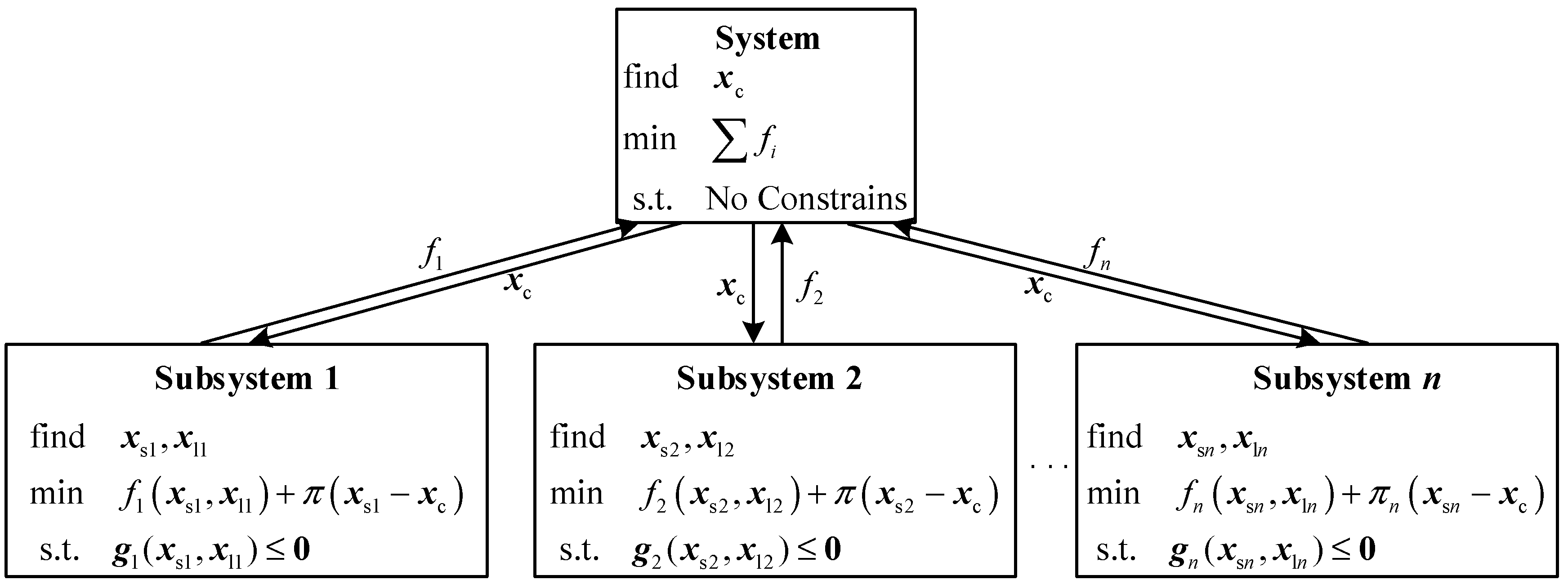
From the analysis of Equation (2), it can be seen that the design objectives f_i and constraints g_i of each structure are coupled through the shared variable x_s. In order to decouple the objective function and constraints of each structure, a coordination variable x_c is introduced, and Equation (2) is transformed into the following form:

$$\begin{array}{lll}\mathrm{find}\hfill & \hfill & ({\mathit{x}}_{\mathrm{c}},{\mathit{x}}_{\mathrm{l}i}) \left(i=1, 2,\cdot \cdot \cdot ,n\right)\hfill \\ \min \hfill & \hfill & F(f_i({\mathit{x}}_{\mathrm{s}i},{\mathit{x}}_{\mathrm{l}i}\left)\right)\hfill \\ \mathrm{s}.\mathrm{t}.\hfill & \hfill & g_i({\mathit{x}}_{\mathrm{s}i},{\mathit{x}}_{\mathrm{l}i})\le \mathbf{0}\hfill \\ \hfill & \hfill & {\mathit{x}}_{\mathrm{s}i}-{\mathit{x}}_{\mathrm{c}}=\mathbf{0}\hfill \end{array}$$

(3)

where x_si is the value of the shared variable in i-th structure after decoupling. Analysis shows that the consistency constraint x_si − x_c = 0 makes Equations (3) and (2) equivalent. Equation (3) takes the structural performance as the objective function and the consistency as the constraint, and the consistency constraint is an equality constraint. In order to deal with the equality consistency constraint, this paper introduces a penalty function π(x_si − x_c) to relax the consistency constraint and adds the penalty function to the design goals of each subsystem. Finally, Equation (3) is decomposed into a two-stage optimization problem, as shown in Figure 2.

4.1. Subsystem Optimization

Each subsystem optimization problem is independent of each other, and the number of subsystem optimization problems is the same as the number of substructures contained in the modular structure. At the subsystem, each substructure is optimized, and its objective function consists of two parts, the structural performance and the penalty function. The mathematical description of the i-th subsystem optimization problem is as follows:

$$\begin{array}{l}\begin{array}{cc}\mathrm{find}& {\mathit{x}}_{\mathrm{s}i},{\mathit{x}}_{\mathrm{l}i}\end{array}\\ \begin{array}{cc}\min & f_i+\end{array}\pi \left({\mathit{x}}_{\mathrm{s}i}-{\mathit{x}}_{\mathrm{c}}\right)\\ \begin{array}{cc} \mathrm{s}.\mathrm{t}.& {\mathit{g}}_i({\mathit{x}}_{\mathrm{s}i},{\mathit{x}}_{\mathrm{l}i})\le \mathbf{0}\end{array}\end{array}$$

(4)

Although the penalty function π makes each subsystem independent, the existence of the penalty function also makes the shared variables have different values in different subsystems, that is, there is a tolerance in the consistency constraint. In order to make each subsystem optimization result meet the consistency requirements, this paper chooses the quadratic penalty function [21] to make the consistency constraint tolerance gradually tend to 0. The expression of the penalty function is as follows:

$$\pi \left({\mathit{x}}_{\mathrm{s}i}-{\mathit{x}}_{\mathrm{c}}\right)={\Vert \mathbf{\kappa }\circ \left({\mathit{x}}_{\mathrm{s}i}-{\mathit{x}}_{\mathrm{c}}\right)\Vert }_2^2$$

(5)

where $\mathbf{\kappa }$ is the penalty parameter vector. $\circ$ means multiplying the corresponding elements of the two vectors. As the iteration progresses, the value of the penalty parameter vector $\mathbf{\kappa }$ is continuously updated and increased, and the updated method is as follows:

$${\mathbf{\kappa }}^{(w+1)}=\{\begin{array}{cc}{\mathbf{\kappa }}^{(w)}& \Vert {\mathit{x}}_{\mathrm{s}i}^{\left(w\right)}-{\mathit{x}}_{\mathrm{c}}^{\left(w\right)}\Vert \le \theta \Vert {\mathit{x}}_{\mathrm{s}i}^{\left(w-1\right)}-{\mathit{x}}_{\mathrm{c}}^{\left(w-1\right)}\Vert \\ \gamma {\mathbf{\kappa }}^{(w)}& \Vert {\mathit{x}}_{\mathrm{s}i}^{\left(w\right)}-{\mathit{x}}_{\mathrm{c}}^{\left(w\right)}\Vert >\theta \Vert {\mathit{x}}_{\mathrm{s}i}^{\left(w-1\right)}-{\mathit{x}}_{\mathrm{c}}^{\left(w-1\right)}\Vert \end{array}$$

(6)

where $\gamma \ge 1$, and $0<\theta <1$. Studies have shown that the optimization converges faster when $2\le \gamma \le 3$ and $\theta =0.25$ [21].

4.2. System Coordination

The system is a very simple, unconstrained optimization problem. It takes the coordination variable x_c as the variable and the sum of the performance of each substructure as the objective function. The system coordinates the value of x_c according to the optimization results of each subsystem to reduce the value of the system objective function and then transmits the coordination result to each subsystem for the next iteration. The mathematical description of system coordination is as follows:

$$\begin{array}{l}{\begin{array}{cc}\mathrm{find}& \mathit{x}\end{array}}_{\mathrm{c}}\\ \begin{array}{cc}\min & {\displaystyle \sum f_i}\end{array}\\ \begin{array}{cc} \mathrm{s}.\mathrm{t}.& \mathrm{No} \mathrm{Constrains}\end{array}\end{array}$$

(7)

The objective function in Equation (4) consists of two parts, the structural performance and the penalty function. The penalty function represents the consistency between the general variable x_si and the coordination variable x_c, and as the value of the penalty parameter vector increases, the penalty function becomes more and more important in the objective function. Therefore, the essence of the objective function in Equation (4) is to gradually sacrifice the performance of the structure so that x_si gradually approaches x_c and finally is completely consistent. Likewise, the system should adjust the value of x_c according to the consistency of x_si and x_c.

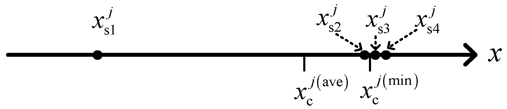
Since the importance of each subsystem is the same, according to the definition of the penalty function, it is easy to know that the essence of the penalty function is the sum of the distances between x_si and x_c. Its minimum value is easy to calculate, but taking the minimum value is not always the best choice. If a certain component of the x_si is distributed in the form shown in Figure 3, then when $x_{\mathrm{c}}^j=x_{\mathrm{c}}^{j\left(\min \right)}$, that is, when $x_{\mathrm{c}}^j$ is between $x_{\mathrm{s}2}^j$ and $x_{\mathrm{s}3}^j$, the penalty function takes the minimum value. At this time, the distance between $x_{\mathrm{c}}^j$ and $x_{\mathrm{s}1}^j$ is too large, and other general variables are gathered in a small range, which is not conducive to the optimization.

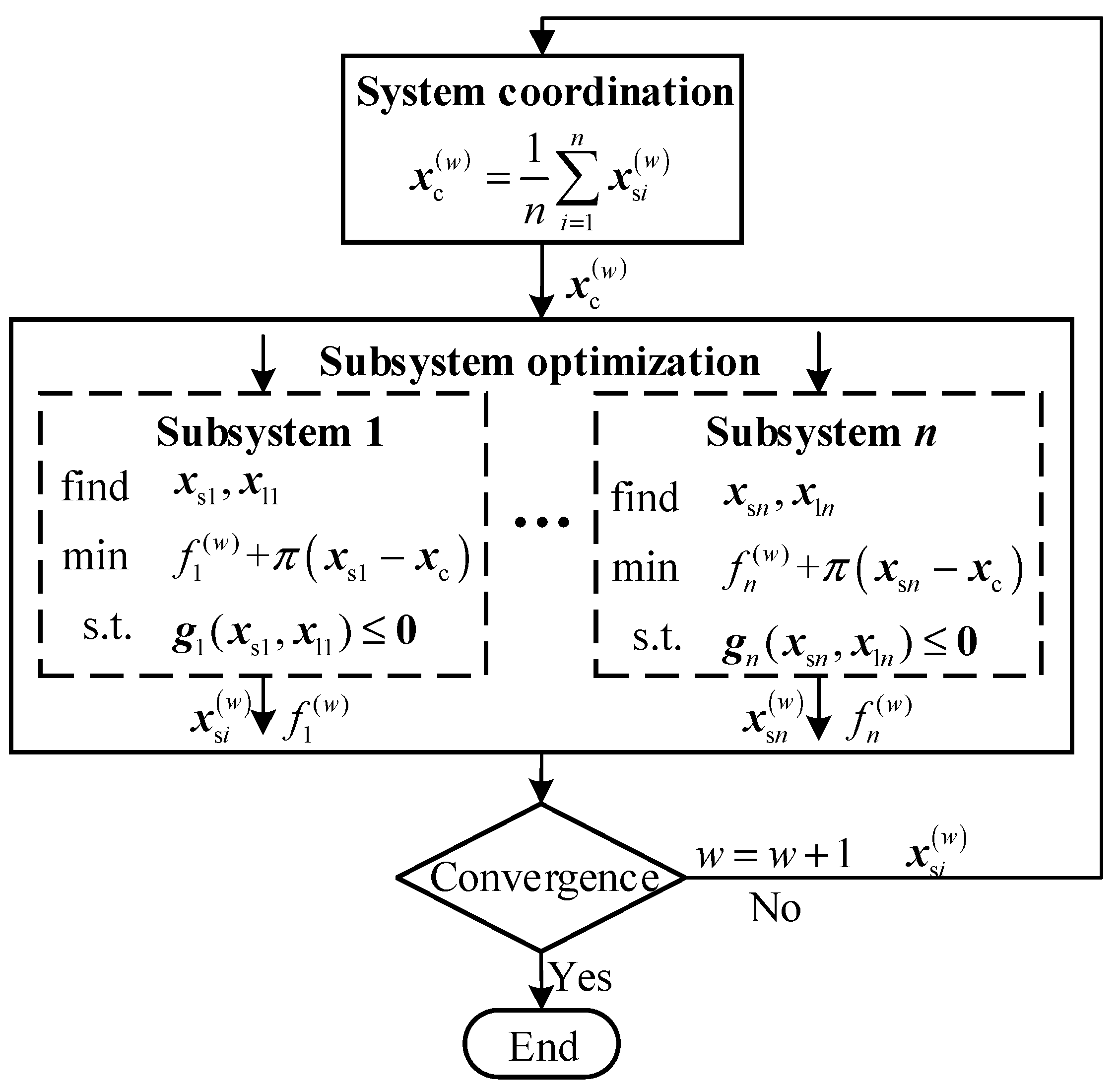
When $x_{\mathrm{c}}^j=x_{\mathrm{c}}^{j\left(\mathrm{ave}\right)}$, that is, when the x_c is equal to the mean value of the x_si of each substructure, the distribution of the x_c and x_si of each substructure is relatively uniform, so let:

$${\mathit{x}}_{\mathrm{c}}=\frac{1}{n}{\displaystyle \sum _{i=1}^n{\mathit{x}}_{\mathrm{s}i}}$$

(8)

where n is the number of substructures contained in the modular structure. Then the system becomes a coordination problem in which the coordination variables are adjusted directly according to the feedback of each subsystem.

4.3. Convergence Analysis

It can be seen from Equation (8) that the x_c is equal to the mean value of the x_si of each substructure. Therefore, when the values of the x_si fed back to the system by each subsystem are different, the value of the x_c will naturally change. On the other hand, as a component of the objective function, the penalty function in Equation (5) will naturally affect the optimization results of each subsystem, and as the iteration progresses, the value of the penalty parameter vector increases continuously, and the penalty function has an increasing influence on the optimization results of each subsystem. The penalty function makes the x_si of each subsystem tend to a certain direction, and this trend will also increase with the increase in the penalty parameter vector. The value of the x_c directly determines the direction, so the x_c will affect the optimization results of each subsystem. This effect will increase as the iteration progresses, and finally the x_si of each structure is consistent with the x_c.

4.4. Stop Condition

There are two stop conditions. The first is that the difference of the sum of the performance in each substructure between the two iteration steps is less than a certain value. The second is that the difference of the x_c between the two iteration steps is less than a certain value.

The first stop condition is shown in Equation (9):

$$\left|({{\displaystyle \sum f_i)}}^{\left(w+1\right)}-({{\displaystyle \sum f_i)}}^{\left(w\right)}\right|\le {\epsilon }_F$$

(9)

where ${\displaystyle \sum f_i}$ is the sum of the performance in each substructure; ${\epsilon }_F$ is the convergence parameter, which is a number greater than 0.

The second stop condition is shown in Equation (10):

$$\max \left|x_{\mathrm{c}}^{j\left(w+1\right)}-x_{\mathrm{c}}^{j\left(w\right)}\right|\le {\epsilon }_{x}j\in \left\{1,2,\dots ,m\right\}$$

(10)

where $x_{\mathrm{c}}^j$ is the j-th component of the x_c; m is the number of variables contained in x_c; and ${\epsilon }_x$ is the convergence parameter of the x_c, which is a number greater than 0.

4.5. Optimization Process

The optimization execution process is divided into five steps:

(A)

Build and initialize the optimization model;

(B)

Transfer coordination variables to subsystems;

(C)

Optimize each subsystem;

(D)

According to the optimization results of each subsystem, determine whether the optimization has converged. If so, the optimization is over; otherwise, go to step E;

(E)

The system updates the values of the coordination variables according to the optimization results of each subsystem and then proceeds to step B.

The framework of the MVPM is shown in Figure 4.

5. Numerical Test

This section will test the MVPM with a typical nonconvex numerical optimization example [22,23,24]. This numerical optimization problem has a unique global optimal solution, and all constraints are valid constraints. There are two purpose of the test: the first is to test the convergence of the MVPM, and the second is to test the optimization efficiency of the MVPM. Since this numerical optimization problem is often used to test multidisciplinary optimization algorithms, the CO method is used as a comparison method in this paper. The numerical optimization problem is formulated as follows:

$$\begin{array}{cc}\hfill \mathrm{find}& \mathit{x}={[x_1,\dots ,x_{14}]}^{\mathrm{T}}\hfill \\ \hfill \min & f=x_1^2+x_2^2\hfill \\ \hfill \mathrm{s}.\mathrm{t}.& g_1=(x_3^{-2}+x_4^2)x_5^{-2}-1\le 0\hfill \\ & g_2=(x_5^2+x_6^{-2})x_7^{-2}-1\le 0\hfill \\ & g_3=(x_8^2+x_9^2)x_{11}^{-2}-1\le 0\hfill \\ & g_4=(x_8^{-2}+x_{10}^2)x_{11}^{-2}-1\le 0\hfill \\ & g_5=(x_{11}^2+x_{12}^{-2})x_{13}^{-2}-1\le 0\hfill \\ & g_6=(x_{11}^2+x_{12}^2)x_{14}^{-2}-1\le 0\hfill \\ & h_1=(x_3^2+x_4^{-2}+x_5^2)x_1^{-2}-1=0\hfill \\ & h_2=(x_5^2+x_6^2+x_7^2)x_2^{-2}-1=0\hfill \\ & h_3=(x_8^2+x_9^{-2}+x_{10}^{-2}+x_{11}^2)x_3^{-2}-1=0\hfill \\ & h_4=(x_{11}^2+x_{12}^2+x_{13}^2+x_{14}^2)x_6^{-2}-1=0\hfill \\ & x_1,\dots ,x_{14}>0\hfill \end{array}$$

(11)

The optimal solution to this numerical optimization problem is x* = [2.84, 3.09, 2.36, 0.76, 0.87, 2.81, 0.94, 0.97, 0.87, 0.8, 1.30, 0.84, 1.76, 1.55]^T, and the optimal value of the objective function is f^* = 17.59.

5.1. The Results of the CO Method

The CO method adopts the decomposition method in [25] in the optimization process. This method decomposes the original problem into a system optimization problem and two subsystem optimization problems. The system takes $x_3,x_4,x_5,x_6,x_7,x_{11}$ as the variables; takes the consistency of each subsystem variables and the system variables and $g_1$,$g_2$ as the constraints; takes the objective function of the original problem as the optimization goal; and takes $h_1$ and $h_2$ as the analysis models. The system optimization problem is shown in Equation (12):

$$\begin{array}{cc}\hfill \mathrm{find}& x_3,x_4,x_5,x_6,x_7,x_{11}\hfill \\ \hfill \min & f=x_1^2+x_2^2\hfill \\ \hfill \mathrm{s}.\mathrm{t}.& g_1=(x_3^{-2}+x_4^2)x_5^{-2}-1\le 0\hfill \\ & g_2=(x_5^2+x_6^{-2})x_7^{-2}-1\le 0\hfill \\ & c_1={\left(x_3-x_3^{(1)}\right)}^2+{\left(x_{11}-x_{11}^{(1)}\right)}^2=0\hfill \\ & c_2={\left(x_6-x_6^{(2)}\right)}^2+{\left(x_{11}-x_{11}^{(2)}\right)}^2=0\hfill \\ & x_3,x_4,x_5,x_6,x_7,x_{11}>0\hfill \\ \hfill \mathrm{Analysis}& x_1^2=x_3^2+x_4^{-2}+x_5^2\hfill \\ & x_2^2=x_5^2+x_6^2+x_7^2\hfill \end{array}$$

(12)

where the superscript in parentheses represents the shared variable in the corresponding subsystem.

Subsystem 1 takes $x_8,x_9,x_{10},x_{11}^{(1)}$ as the variables; takes $g_3$ and $g_4$ as the constraints; takes the system consistency constraint $c_1$ as the objective function; and takes $h_3$ as the analytical model. The optimization problem of subsystem 1 is shown in Equation (13):

$$\begin{array}{cc}\hfill \mathrm{find}& x_8,x_9,x_{10},x_{11}^{\left(1\right)}\hfill \\ \hfill \min & c_1={\left(x_3^{(1)}-x_3\right)}^2+{\left(x_{11}^{(1)}-x_{11}\right)}^2\hfill \\ \hfill \mathrm{s}.\mathrm{t}.& g_3=(x_8^2+x_9^2){\left(x_{11}^{\left(1\right)}\right)}^{-2}-1\le 0\hfill \\ \hfill & g_4=(x_8^{-2}+x_{10}^2){\left(x_{11}^{\left(1\right)}\right)}^{-2}-1\le 0\hfill \\ \hfill & x_8,x_9,x_{10},x_{11}^{\left(1\right)}>0\hfill \\ \hfill \mathrm{Analysis}& {\left(x_3^{\left(1\right)}\right)}^2=x_8^2+x_9^{-2}+x_{10}^{-2}+{\left(x_{11}^{\left(1\right)}\right)}^2\hfill \end{array}$$

(13)

Subsystem 2 takes $x_{11}^{(2)},x_{12},x_{13},x_{14}$ as the variables; takes $g_5$ and $g_6$ as the constraints; takes the system consistency constraint $c_2$ as the objective function; and takes $h_4$ as the analytical model. The optimization problem of subsystem 2 is shown in Equation (14):

$$\begin{array}{ll}\hfill \mathrm{find}& x_{11}^{\left(2\right)},x_{12},x_{13},x_{14}\hfill \\ \hfill \min & c_1={\left(x_6^{(2)}-x_6\right)}^2+{\left(x_{11}^{(2)}-x_{11}\right)}^2\hfill \\ \hfill \mathrm{s}.\mathrm{t}.& g_5=({\left(x_{11}^{(2)}\right)}^2+x_{12}^{-2})x_{13}^{-2}-1\le 0\hfill \\ \hfill & g_6=({\left(x_{11}^{(2)}\right)}^2+x_{12}^2)x_{14}^{-2}-1\le 0\hfill \\ \hfill & x_{11}^{\left(2\right)},x_{12},x_{13},x_{14}>0\hfill \\ \hfill \mathrm{Analysis}& {\left(x_6^{\left(2\right)}\right)}^2={\left(x_{11}^{\left(2\right)}\right)}^2+x_{12}^2+x_{13}^2+x_{14}^2\hfill \end{array}$$

(14)

Select x₁ = [2.00, 2.00,…, 2.00]T, x₂ = [3.00, 3.00,…, 3.00]T and x₃ = [4.00, 4.00,…, 4.00]T as initial points, respectively. Both system and subsystem use sequential quadratic programming algorithms. The optimization results are shown in

Table 1. The results of the CO.

Initial Points	Results	Target Value	Iterations Number
x1	[2.80, 3.15, 2.38, 0.95, 1.04, 2.77, 1.10, 0.97, 0.85, 0.77, 1.28, 0.85, 1.73, 1.53]T	17.80	140
x2	[2.96, 2.99, 2.38,0.63, 0.76, 2.77, 0.84, 0.97, 0.84, 0.77, 1.28, 0.85, 1.73, 1.53]T	17.68	121
x3	[2.82, 3.10, 2.30, 0.71, 0.84, 2.84, 0.91, 0.96, 0.93, 0.84, 1.33, 0.85, 1.77, 1.57]T	17.53	174

.

It can be found from Table 1 that the CO method requires many iterations to complete the optimization, that is, the efficiency of the CO is low. For different optimization initial points, there is a certain gap in the final optimization results, that is, the stability of the CO is poor.

5.2. The Results of the MVPM Method

The MVPM takes $x_3,x_4,x_5,x_6,x_7,x_{11}$ as the variables of the general module; takes $x_1,x_8,x_9,x_{10}$ as the variables of the dedicated module 1; and takes $x_2,x_{12},x_{13},x_{14}$ as the variables of the dedicated module 2. The original objective function is split into two parts, as shown in Equation (15):

$$\begin{array}{cc}\hfill {\mathit{x}}_{\mathrm{c}}& ={[x_3,x_4,x_5,x_6,x_7,x_{11}]}^{\mathrm{T}}\hfill \\ \hfill {\mathit{x}}_{\mathrm{s}1}& ={[x_3^{(1)},x_4^{(1)},x_5^{(1)},x_6^{(1)},x_7^{(1)},x_{11}^{(1)}]}^{\mathrm{T}}\hfill \\ \hfill {\mathit{x}}_{11}& ={[x_1,x_8,x_9,x_{10}]}^{\mathrm{T}}\hfill \\ \hfill {\mathit{x}}_{\mathrm{s}2}& ={[x_3^{(2)},x_4^{(2)},x_5^{(2)},x_6^{(2)},x_7^{(2)},x_{11}^{(2)}]}^{\mathrm{T}}\hfill \\ \hfill {\mathit{x}}_{12}& ={[x_2,x_{12},x_{13},x_{14}]}^{\mathrm{T}}\hfill \\ \hfill f_1& =x_1^2\hfill \\ \hfill f_2& =x_2^2\hfill \end{array}$$

(15)

The original problem is then decomposed into a system and two subsystem optimization problems. The system is an unconstrained coordination problem. Take $h_1$ and $h_2$ as the analysis model of subsystem 1 and subsystem 2, respectively. The system coordination problem is as follows:

$${\mathit{x}}_{\mathrm{c}}=\frac{1}{2}\left({\mathit{x}}_{\mathrm{s}1}+{\mathit{x}}_{\mathrm{s}2}\right)$$

(16)

Subsystem 1 takes $g_2,g_3,g_4,h_3$ as the constraints and takes $h_1$ as the analysis model. The subsystem 1 is as follows:

$$\begin{array}{cc}\hfill \mathrm{find}& {\mathit{x}}_{\mathrm{s}1},{\mathit{x}}_{\mathrm{l}1}\hfill \\ \hfill \min & f_1+\pi \left({\mathit{x}}_{\mathrm{s}1}-{\mathit{x}}_{\mathrm{c}}\right)\hfill \\ \hfill \mathrm{s}.\mathrm{t}.& g_2=({\left(x_5^{(1)}\right)}^2+{\left(x_6^{(1)}\right)}^{-2}){\left(x_7^{(1)}\right)}^{-2}-1\le 0\hfill \\ & g_3=(x_8^2+x_9^2){\left(x_{11}^{(1)}\right)}^{-2}-1\le 0\hfill \\ & g_4=(x_8^{-2}+x_{10}^2){\left(x_{11}^{(1)}\right)}^{-2}-1\le 0\hfill \\ & h_3=(x_8^2+x_9^{-2}+x_{10}^{-2}+{\left(x_{11}^{(1)}\right)}^2){\left(x_3^{(1)}\right)}^{-2}-1=0\hfill \\ & {\mathit{x}}_{\mathrm{s}1}, {\mathit{x}}_{11}>\mathbf{0}\hfill \\ \hfill \mathrm{Analysis} & x_1^2={\left(x_3^{(1)}\right)}^2+{\left(x_4^{(1)}\right)}^{-2}+{\left(x_5^{(1)}\right)}^2\hfill \end{array}$$

(17)

Subsystem 2 takes $g_1,g_5,g_6,h_4$ as the constraints and takes $h_2$ as the analysis model. The subsystem 2 is as follows:

$$\begin{array}{cc}\hfill \mathrm{find}& {\mathit{x}}_{\mathrm{s}2},{\mathit{x}}_{\mathrm{l}2}\hfill \\ \min & f_2+\pi \left({\mathit{x}}_{\mathrm{s}2}-{\mathit{x}}_{\mathrm{c}}\right)\hfill \\ \hfill \mathrm{s}.\mathrm{t}.& g_1=({\left(x_3^{(2)}\right)}^{-2}+{\left(x_4^{(2)}\right)}^2){\left(x_5^{(2)}\right)}^{-2}-1\le 0\hfill \\ & g_5=({\left(x_{11}^{(2)}\right)}^2+x_{12}^{-2})x_{13}^{-2}-1\le 0\hfill \\ & g_6=({\left(x_{11}^{(2)}\right)}^2+x_{12}^2)x_{14}^{-2}-1\le 0\hfill \\ & h_4=({\left(x_{11}^{(2)}\right)}^2+x_{12}^2+x_{13}^2+x_{14}^2){\left(x_6^{(2)}\right)}^{-2}-1=0\hfill \\ & {\mathit{x}}_{\mathrm{s}2}, {\mathit{x}}_{12}>\mathbf{0}\hfill \\ \mathrm{Analysis}\hfill & x_2^2={\left(x_5^{(2)}\right)}^2+{\left(x_6^{(2)}\right)}^2+{\left(x_7^{(2)}\right)}^2\hfill \end{array}$$

(18)

Pick the same three points as the CO method: x₁ = [2.00, 2.00,…, 2.00]^T, x₂ = [3.00, 3.00,…, 3.00]^T and x₃ = [4.00, 4.00,…, 4.00]^T as the initial points, and let the optimization parameter κ = [0.1, 0.1,…, 0.1]^T, γ = 2, 𝜃 = 0.25. The results are shown in

Table 2. The results of the MVPM.

Initial Points	Results	Target Value	Iterations Number
x1	[3.35, 2.69, 2.64, 0.51, 0.63, 2.46, 0.75, 0.99, 0.68, 0.65, 1.14, 0.84, 1.62, 1.39]T	18.43	17
x3	[3.36, 2.74, 2.66, 0.51, 0.64, 2.54, 0.75, 0.99, 0.67, 0.64, 1.15, 0.84, 1.63, 1.39]T	18.77	20
x4	[3.32, 2.68, 2.62, 0.52, 0.64, 2.46, 0.75, 0.99, 0.68, 0.65, 1.13, 0.84, 1.59, 1.35]T	18.16	16

.

It can be found from Table 2 that, compared with the CO method, the MVPM method requires fewer iterations to complete the optimization, and for different initial points, the final results of the are more stable.

5.3. Numerical Test Summary

The results obtained by the two optimization methods are summarized in

Table 3. Comparison of two results.

Method	Dispersion	Target Value	Iterations Number
CO	0.41	17.67	145
MVPM	0.10	18.45	18

.

The dispersion in Table 3 is the sum of the Euclidean distances of each two results, and its value is equal to the sum of the square-norm of the difference between the result vectors. The calculation formula is:

$${\Vert {\mathit{x}}_1^{*}-{\mathit{x}}_2^{*}\Vert }_2+{\Vert {\mathit{x}}_1^{*}-{\mathit{x}}_3^{*}\Vert }_2+{\Vert {\mathit{x}}_2^{*}-{\mathit{x}}_3^{*}\Vert }_2$$

(19)

Comparing the two results, it can be seen that the optimization effect of the CO method is better, but its efficiency is low and requires a lot of iterations to converge. The main reason is that the system consistency constraints of the CO method need to be obtained by calling subsystem optimization so that each analysis at the system needs to call a complete subsystem optimization. In contrast, the gradient information obtained by difference at the system is easily overwhelmed by the error of subsystem optimization, which makes it difficult for the algorithm to converge. This is also the main reason for the large dispersion of the results of the collaborative optimization method.

Compared with the CO method, the efficiency of the MVPM method is higher. The main reason is that each iteration of the MVPM method only needs to call the subsystem once. In terms of optimization effect, since the system of MVPM method is a coordination problem, its optimization effect is not as good as that of CO method, but it is also closer to the global best.

6. Wing Structure Design of Modular UAV

In this section, the MVPM is applied to the structural layout design of a modular aircraft wing, and the difference between the structural layout of the general module and the dedicated module in the general design and the individual design is analyzed. This example provides guidance for the structural layout optimization of modular aircraft.

6.1. Structural Description

It is becoming more and more expensive to develop a new type of aircraft due to increased requirements, and designing a separate aircraft for each mission would make the design cost unacceptable. Funk et al. (2006) believe that future military aircraft must be flexible enough. Modular aircraft can be replaced by different dedicated modules to accomplish different tasks, and it is easy to design a new dedicated module to meet the newly added requirements. Modular aircraft have high flexibility and can also reduce the life cycle cost of the aircraft. Therefore, modular aircraft have broad application prospects.

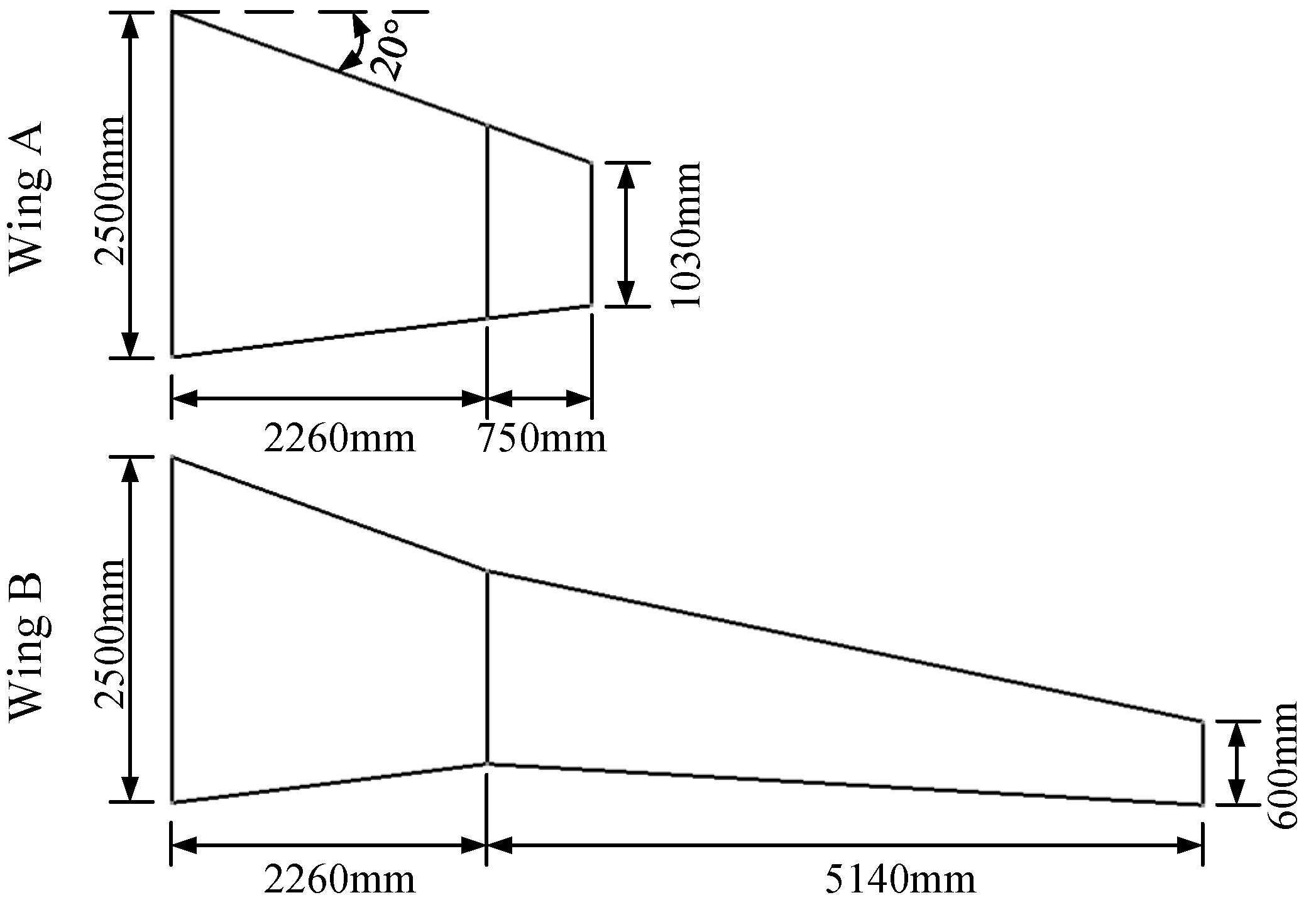
In order to increase the functional diversity of UAV and reduce the design and manufacturing cost, this section takes MQ-X UAV as the prototype and designs a modular UAV including model A and model B. The wings of the two types of UAVs adopt a modular design. The A-type UAV has a small wingspan and strong maneuverability and is mainly used for attack missions. The B-type UAV has a larger wingspan, longer flight time and higher flight altitude and is mainly used for reconnaissance and surveillance missions. The wing is composed of inner and outer sections, of which the inner section is a general module, and the outer section is a dedicated module, as shown in Figure 5.

The swept angle of the leading edge of the inner wing is 20 degrees. The leading and trailing edges of the outer section of the A-type wing coincide with the inner section. The leading edge sweep of the outer section of the B-type wing is 12 degrees. Due to the different uses of the two types of aircraft, the loads of the two types of aircraft are different. The basic data of the two aircrafts are shown in

Table 4. The basic data of the modular aircraft.

Type	Maximum Takeoff Weight/kg	Wingspan/m	Overload/G	Fuselage Width/m	Cruising Altitude/km	Cruising Speed/Mach
A	2700	8.02	10.00	2.00	7.00	0.80
B	3000	16.8	2.50	2.00	12.00	0.23

.

It is assumed that all the lift of the aircraft is provided by the wings, and the unloading effect of the wing structure’s own weight is ignored. Therefore, the total load on a single wing is M_A = 135,000 N and M_B =37,500 N.

It is assumed that the aerodynamic load is triangularly distributed along the wing chord and takes the maximum value at 20% of the chord length. The distribution of aerodynamic load along the span wise is trapezoidal, and the magnitude of the load at each span wise position is proportional to the chord length. The span wise load is shown in Equation (20):

$$W\left(y\right)=\frac{2M}{\left(c_{\mathrm{R}}+c_{\mathrm{T}}\right)\times b}\times \left[c_{\mathrm{R}}-\left(c_{\mathrm{R}}-c_{\mathrm{T}}\right)\times \frac{y}{b}\right]$$

(20)

where W(y) is the span wise distribution of aerodynamic loads; $c_{\mathrm{R}}$ and $c_{\mathrm{T}}$ are the root chord length and tip chord length, respectively; y is the span wise coordinate; b is the span wise length of the one-side wing; and M is the total load on the one-side wing.

6.2. Optimization Model

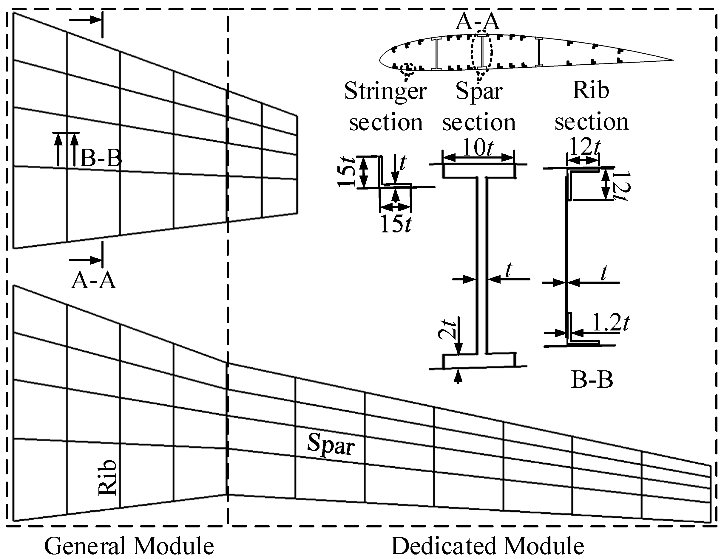
As shown in Figure 6, the wing consists of spars, ribs, skins and stringers. In the wing optimization model, the variables include layout variables and dimensional variables, and the layout variables include discrete variables and position variables.

In the inner wing, the layout design variables use the number of spars and ribs as discrete variables and the chord wise percent position of each spar as the location variable. The outer wing has the same number and position of spars as the inner wing. The ribs of the inner wing are evenly distributed, and the number of ribs of the outer wing is fixed. In the outer wing, the A-type wing has three ribs, and the B-type wing has eight ribs.

Dimensional variables include the dimensions of spars, ribs and skins. In order to simplify the optimization model, the dimensions of the spar, rib and skin vary linearly along the span wise direction of the wing, and the dimensions of the four sections of the inner wing root, inner wing tip, outer wing root and outer wing tip are taken as variables, respectively. The thickness of the upper and lower skins of the wing is the same, and the thickness is equal along the chord direction. The rib is composed of a web and a flange. The thickness of the rib web is uniform. The cross-section of the flange is L-shaped. The thickness of the flange is equal to 1.2 times the thickness of the web, and the width and height are equal to 12 times the thickness of the web. Take the thickness of the rib web as variable. The spar consists of a web and a flange. The web thickness changes linearly along the span wise. The cross-section of the flange is rectangular, the thickness of the flange is equal to 2 times the thickness of the web, and the width is equal to 10 times the thickness of the web. Take the thickness of the spar web as variable. In addition, there are three stringers before the front spar, behind the rear spar and between each spar. The section of the stringer is L-shaped, and the dimensions of the stringer vary linearly along the span wise. Since the main function of the stringer is to strengthen the stability of the skin, it is a secondary component of the wing. Therefore, the thickness of the stringer is equal to 1.2 times the thickness of the skin, and the width and height are equal to 18 times the thickness of the skin. The symbols and value ranges of the variables are shown in

Table 5. Symbols and value ranges of variables.

Type	Item/Units	Symbol	Range
layout variables	Number of spars	spar_num	2, 3
	Position of spars	spar_locationi	0.1~0.7
	Number of inner ribs	rib_num_in	3, 4, 5, 6
dimension variables	Root web thickness of inner wing spar/mm	spar_size_in_rooti	2.0~10.0
	Top web thickness of inner wing spar/mm	spar_size_in_topi	0.8~5.0
	Root web thickness of outer wing spar/mm	spar_size_out_rooti,j	1.0~6.0
	Top web thickness of outer wing spar/mm	spar_size_out_topi,j	0.8~4.0
	Root thickness of inner wing skin/mm	skin_size_in_root	0.8~4.0
	Top thickness of inner wing skin/mm	skin_size_in_top	0.8~4.0
	Root thickness of outer wing skin/mm	skin_size_out_rootj	0.8~4.0
	Top thickness of outer wing skin/mm	skin_size_out_topj	0.8~4.0
	Web thickness of root rib of inner wing/mm	rib_size_in_root	0.8~4.0
	Web thickness of top rib of inner wing/mm	rib_size_in_top	0.8~4.0
	Web thickness of root rib of outer wing/mm	rib_size_out_rootj	0.8~4.0
	Web thickness of top rib of outer wing/mm	rib_size_out_topj	0.8~4.0
constraints	Structural stress/MPa	stressj	−300~300
	Spar spacing	spar_locationj	0.2~0.6
	Spar dimension ratio	spar_sizej	0.5~2

.

$${\mathit{x}}_{\mathrm{s}}=\left[\begin{array}{l}spar\_num\\ spar\_locatio{n}_1\\ spar\_locatio{n}_2\\ spar\_locatio{n}_3\\ rib\_num\_in\\ spar\_size\_in\_roo{t}_1\\ spar\_size\_in\_roo{t}_2\\ spar\_size\_in\_roo{t}_3\\ spar\_size\_in\_to{p}_1\\ spar\_size\_in\_to{p}_2\\ spar\_size\_in\_to{p}_3\\ skin\_size\_in\_root\\ skin\_size\_in\_top\\ rib\_size\_in\_root\\ rib\_size\_in\_top\end{array}\right]{\mathit{x}}_{\mathrm{lA}}=\left[\begin{array}{l}spar\_size\_out\_roo{t}_{1,A}\\ spar\_size\_out\_roo{t}_{2,A}\\ spar\_size\_out\_roo{t}_{3,A}\\ spar\_size\_out\_to{p}_{1,A}\\ spar\_size\_out\_to{p}_{2,A}\\ beam\_size\_out\_to{p}_{3,A}\\ skin\_size\_out\_roo{t}_A\\ skin\_size\_out\_to{p}_{\mathrm{A}}\\ rib\_size\_out\_roo{t}_{\mathrm{A}}\\ rib\_size\_out\_to{p}_{\mathrm{A}}\end{array}\right]{\mathit{x}}_{\mathrm{lB}}=\left[\begin{array}{l}spar\_size\_out\_roo{t}_{1,\mathrm{B}}\\ spar\_size\_out\_roo{t}_{2,\mathrm{B}}\\ spar\_size\_out\_roo{t}_{3,\mathrm{B}}\\ spar\_size\_out\_to{p}_{1,\mathrm{B}}\\ spar\_size\_out\_to{p}_{2,\mathrm{B}}\\ spar\_size\_out\_to{p}_{3,\mathrm{B}}\\ skin\_size\_out\_roo{t}_{\mathrm{B}}\\ skin\_size\_out\_to{p}_{\mathrm{B}}\\ rib\_size\_out\_roo{t}_{\mathrm{B}}\\ rib\_size\_out\_to{p}_{\mathrm{B}}\end{array}\right]$$

(21)

The value of the subscript j takes A and B, representing wing A and wing B, respectively. When the number of spars is equal to 3, the value of the subscript i is equal to 1, 2 or 3, representing the front, middle and rear spars, respectively. When the number of spars is equal to 2, the value of the subscript i is equal to 1 or 2, representing the front and rear spars, respectively. In constraints, the spar spacing represents the ratio of the distance between adjacent spars to the chord length, which is used to ensure that the spar spacing is not too small or too large. The spar dimension ratio represents the ratio of different spar dimensions, which is used to ensure that the difference between different spar dimensions is not too large.

The variables of general modules are shared variables, and the variables of dedicated modules are local variables. Shared variables and local variables are listed in Equation (21).

It is assumed that the materials used for the wings are all duralumin alloys. The material modulus is 70 GPa, and the density is 2700 kg/m³. Taking the structural weight as the objective function, when the generality is not considered and each wing is optimized individually, the optimization model is as follows:

$$\begin{array}{cc}\begin{array}{r}\hfill \mathrm{find}\\ \hfill \min \\ \hfill \mathrm{s}.\mathrm{t}.\\ \hfill \\ \hfill \end{array}& \begin{array}{l}{\mathit{x}}_{\mathrm{s}},{\mathit{x}}_{\mathrm{l}j}\hfill \\ M_j\hfill \\ -300\mathrm{MPa}\le stres{s}_j\le 300\mathrm{MPa}\hfill \\ 0.2\le spar\_locatio{n}_j\le 0.6\hfill \\ 0.5\le spar\_siz{e}_j\le 2\hfill \end{array}\end{array}$$

(22)

where the value of j is equal to A or B, representing wing A and wing B, respectively. $M_j$ is the mass of wing A or wing B.

When the general design is adopted, the total mass of the two wing structures is used as the objective function, and each wing structure should satisfy the corresponding constraints at the same time. The optimization model is as follows:

$$\begin{array}{cc}\begin{array}{r}\hfill \mathrm{find}\\ \hfill \min \\ \hfill \mathrm{s}.\mathrm{t}.\\ \hfill \\ \hfill \\ \hfill \\ \hfill \\ \hfill \end{array}& \begin{array}{l}{\mathit{x}}_{\mathrm{s}},{\mathit{x}}_{\mathrm{lA}},{\mathit{x}}_{\mathrm{lB}}\hfill \\ M_{\mathrm{A}}+M_{\mathrm{B}}\hfill \\ -300\mathrm{MPa}\le stres{s}_{\mathrm{A}}\le 300\mathrm{MPa}\hfill \\ -300\mathrm{MPa}\le stres{s}_{\mathrm{B}}\le 300\mathrm{MPa}\hfill \\ 0.2\le spar\_locatio{n}_{\mathrm{A}}\le 0.6\hfill \\ 0.2\le spar\_locatio{n}_{\mathrm{B}}\le 0.6\hfill \\ 0.5\le spar\_siz{e}_{\mathrm{A}}\le 2\hfill \\ 0.5\le spar\_siz{e}_{\mathrm{B}}\le 2\hfill \end{array}\end{array}$$

(23)

6.3. Results and Discussion

In order to analyze the weight increase in each wing after the general design is adopted, each wing is independently optimized first. During the optimization process, an approximate model [26,27] is used instead of finite element analysis. During the construction of the approximate model, the optimal Latin hypercube algorithm and the second-order response surface model were used, and the reliability of the response surface was controlled (R-Squared > 0.998). Finally, the MOST algorithm [28] is selected for optimization, and the results are shown in

Table 6. Individual optimization results.

Item	Symbol	Wing A	Wing B
Number of spars	spar_num	3	3
Position of spars	spar_location1	0.203	0.207
	spar_location2	0.403	0.407
	spar_location3	0.603	0.607
Number of inner ribs	rib_num_in	6	4
Root web thickness of inner wing spar/mm	spar_size_in_root1	3.582	2.000
	spar_size_in_root2	7.164	3.804
	spar_size_in_root3	3.582	2.000
Top web thickness of inner wing spar/mm	spar_size_in_top1	0.800	0.800
	spar_size_in_top2	0.800	1.281
	spar_size_in_top3	0.800	0.807
Root thickness of inner wing skin/mm	skin_size_in_root	1.150	1.126
Top thickness of inner wing skin/mm	skin_size_in_top	0.800	1.363
Web thickness of root rib of inner wing/mm	rib_size_in_root	0.800	0.800
Web thickness of top rib of inner wing/mm	rib_size_in_top	0.800	0.800
Root web thickness of outer wing spar/mm	spar_size_out_root1	1.000	1.000
	spar_size_out_root2	1.000	1.000
	spar_size_out_root3	1.000	1.000
Top web thickness of outer wing spar/mm	spar_size_out_top1	0.800	0.800
	spar_size_out_top2	0.800	0.800
	spar_size_out_top3	0.800	0.800
Root thickness of outer wing skin/mm	skin_size_out_root	0.800	1.399
Top thickness of outer wing skin/mm	skin_size_out_top	0.800	0.800
Web thickness of root rib of outer wing/mm	rib_size_out_root	0.800	0.800
Web thickness of top rib of outer wing/mm	rib_size_out_top	0.800	0.800
Mass/kg	M	48.151	76.358

.

The M in Table 6 is the structural weight of the single-sided wing. Unless otherwise specified, the mass described in this chapter is the weight of the single-sided wing. When the generality is not considered, the optimal layout and dimension of the general module in the two wings are quite different. Wing A has a smaller area and a larger aerodynamic load, so more ribs and thicker skin are required to carry the aerodynamic load. Relatively speaking, the type B wing has a larger wing area and smaller aerodynamic load, so it has a smaller number of ribs and a smaller thickness of the skin.

In the general design process, an approximate model [26,27] is used instead of finite element analysis. During the construction of the approximate model, the optimal Latin hypercube algorithm and the second-order response surface model were used, and the reliability of the response surface was controlled (R-Squared > 0.998). We set the optimization parameters κ = [0.7,0.7,…,0.7]^T, γ = 2 and 𝜃 = 0.25. Finally, the MOST algorithm is selected for optimization, and the results are shown in

Table 7. General optimization results.

Item	Symbol	Wing A	Wing B
Number of spars	spar_num	3	3
Position of spars	spar_location1	0.204	0.204
	spar_location2	0.404	0.404
	spar_location3	0.604	0.604
Number of inner ribs	rib_num_in	5	5
Root web thickness of inner wing spar/mm	spar_size_in_root1	3.090	3.090
	spar_size_in_root2	6.174	6.174
	spar_size_in_root3	3.091	3.091
Top web thickness of inner wing spar/mm	spar_size_in_top1	0.803	0.803
	spar_size_in_top2	1.047	1.047
	spar_size_in_top3	0.800	0.800
Root thickness of inner wing skin/mm	skin_size_in_root	1.371	1.371
Top thickness of inner wing skin/mm	skin_size_in_top	1.343	1.343
Web thickness of root rib of inner wing/mm	rib_size_in_root	0.800	0.800
Web thickness of top rib of inner wing/mm	rib_size_in_top	0.800	0.800
Root web thickness of outer wing spar/mm	spar_size_out_root1	1.000	1.000
	spar_size_out_root2	1.000	1.000
	spar_size_out_root3	1.000	1.000
Top web thickness of outer wing spar/mm	spar_size_out_top1	0.800	0.800
	spar_size_out_top2	0.800	0.800
	spar_size_out_top3	0.800	0.800
Root thickness of outer wing skin/mm	skin_size_out_root	0.800	1.467
Top thickness of outer wing skin/mm	skin_size_out_top	0.800	0.800
Web thickness of root rib of outer wing/mm	rib_size_out_root	0.800	0.800
Web thickness of top rib of outer wing/mm	rib_size_out_top	0.800	0.800
Mass/kg	M	53.969	86.009
Mass increase/%		12.08	12.64

.

Compared with the individual optimization results of each wing, the number of spar and the position of the spar are basically unchanged, but the number and size of other components have changed to some extent. When wing A is individually optimized, the inner wing has a larger number of ribs and a larger spar dimension, but the skin thickness of the wing tip is smaller. When the general design is adopted, the inner wing of wing A needs to bear the bending moment transmitted by the outer wing of wing B. Therefore, it is necessary to increase the thickness of the skin at the tip of the inner wing while reducing the number of ribs and the dimension of the spar, so that the wing structure maintains strength, and reducing structural weight. Similar results can be obtained when we compare the difference between the inner wing of wing B when it is optimized individually and when it is designed with generality. When wing B is individually optimized, the inner wing has fewer ribs and smaller spar dimensions, but the skin thickness at the wing tip is larger. When the general design is adopted, the inner wing of wing B needs to bear the aerodynamic load of wing A. Therefore, it is necessary to increase the number of ribs and the dimension of the wing spar while reducing the thickness of the skin at the inner wing tip, so that the wing structure maintains strength, and reducing structural weight. When the general design is adopted, the skin thickness of the outer wing root of wing B also increases, which shows that the inner wing and the outer wing structure interact with each other and cannot be designed separately.

When the general design is adopted, the weights of the two wing structures are increased by 5.818 kg/12.08% and 9.651 kg/12.64%, respectively. Although the general design brings the wing a certain weight increase and affects the performance of the aircraft, it also brings higher flexibility and reduces the design and manufacturing costs of the UAV.

7. Conclusions

This paper firstly introduced the layout optimization problem of modular structure and abstracted the mathematical model. Aiming at the problem that the conventional structural layout optimization method is difficult to apply to the modular aircraft structure, this paper drew on the CO method and proposed the MVPM. Then the MVPM method was introduced in detail in the aspects of construction process, system, subsystem, convergence conditions and optimization process.

In this paper, a typical nonconvex numerical optimization example was used to test the MVPM method, and the CO method was selected as the comparison. The results show that the MVPM has high efficiency and high stability. Finally, this chapter takes the application of the MVPM in the layout optimization problem of a modular UAV wing structure as an example and shows the feasibility of the MVPM to solve the optimization problem of modular structure layout and provides a feasible method for the layout design of modular structure.

References

- Simpson, T.W. A Concept Exploration Method for Product Family Design; Georgia Institute of Technology: Atlanta, GA, USA, 1998. [Google Scholar]
- Muffatto, M. Introducing a platform strategy in product development. Int. J. Prod. Econ. 1999, 60–61, 145–153. [Google Scholar] [CrossRef]
- Willcox, K.; Wakayama, S. Simultaneous optimization of a multiple-aircraft family. J. Aircr. 2003, 40, 616–622. [Google Scholar] [CrossRef]
- Meyer, M.H.; Lehnerd, A.P. The Power of Product Platforms; Free Press: New York, NY, USA, 1997. [Google Scholar]
- Simpson, T.W.; Jiao, J.; Siddique, Z.; Hölttä-Otto, K. Advances in Product Family and Product Platform Design; Springer: New York, NY, USA, 2014. [Google Scholar]
- Simpson, T.W.; Siddique, Z.; Jiao, J.R. Product Platform and Product Family Design; Springer: New York, NY, USA, 2006. [Google Scholar]
- Jiao, J.; Simpson, T.W.; Siddique, Z. Product family design and platform-based product development: A state-of-the-art review. J. Intell. Manuf. 2007, 18, 5–29. [Google Scholar] [CrossRef]
- Simpson, T.W. Product platform design and customization: Status and promise. Ai Edam-Artif. Intell. Eng. Des. Anal. Manuf. 2004, 18, 3–20. [Google Scholar] [CrossRef]
- Uddin, Z.; Harland, P.E.; Yörür, H. Risk management in product platform development projects. Int. J. Prod. Dev. 2018, 22, 441–463. [Google Scholar] [CrossRef]
- Fellini, R.; Kokkolaras, M.; Papalambros, P.Y. Quantitative platform selection in optimal design of product families, with application to automotive engine design. J. Eng. Des. 2006, 17, 429–446. [Google Scholar] [CrossRef]
- Ulrich, K.T.; Eppinger, S.D. Product Design and Development; Tata McGraw-Hill Education: New York, NY, USA, 2004. [Google Scholar]
- Rajan, S.D. Sizing, Shape, and Topology Design Optimization of Trusses Using Genetic Algorithm. J. Struct. Eng. 1995, 121, 1480–1487. [Google Scholar] [CrossRef]
- Duan, B.Y.; Ye, S.H. A mixed method for shape optimization of skeletal structures. Eng. Optim. 1986, 10, 183–197. [Google Scholar]
- Hasancebi, O.; Erbatur, F. Layout optimization of trusses using improved GA methodologies. Acta Mech. 2001, 146, 87–107. [Google Scholar] [CrossRef]
- Saka, M.P. Shape optimization of trusses. J. Struct. Div. 1980, 106, 1155–1174. [Google Scholar] [CrossRef]
- Bendsøe, M.P.; Ben-Tal, A.; Haftka, R.T. New displacement-based methods for optimal truss topology design. In Proceedings of the 32nd AIAA/ASME/ASCE/AHS/ASC Structures, Structural Dynamics and Materials Conference, Baltimore, MD, USA, 4–9 May 2009; pp. 684–696. [Google Scholar]
- Sankaranarayanan, S.; Haftka, R.T.; Kapania, R.K. Truss topology optimization with stress and displacement constraints. In Topology Design of Structures; Springer: Dordrecht, The Netherlands, 1993; pp. 71–78. [Google Scholar]
- Sobieszczanski-Sobieski, J. A Linear Decomposition Method for Large Optimization Problems. NASA TM: 83248. 1982. Available online: https://ntrs.nasa.gov/citations/19820014371 (accessed on 1 February 1982).
- Nayak, R.U.; Chen, W.; Simpson, T.W. A variation-based method for product family design. Eng. Optim. 2002, 34, 65–81. [Google Scholar] [CrossRef]
- Braun, R.; Kroo, I. Development and application of the collaborative optimization architecture in a multidisciplinary design environment. In Multidisciplinary Design Optimization: State of the Art; SIAM: Philadelphia, PA, USA, 1995; pp. 98–116. [Google Scholar]
- Dimitri, B. Nonlinear Programming; Athena Scientific: Cambridge, MA, USA, 2016. [Google Scholar]
- Tosserams, S.; Etman, L.F.P.; Rooda, J.E. An augmented Lagrangian decomposition method for quasi-separable problems in MDO. Struct. Multidiscip. Optim. 2007, 34, 211–227. [Google Scholar] [CrossRef]
- Kim, H.M. Target Cascading in Optimal System Design; University of Michigan: Ann Arbor, MI, USA, 2001. [Google Scholar]
- Kroo, I.; Roth, B.D. Enhanced collaborative optimization: A decomposition-based method for multidisciplinary design. In Proceedings of the ASME 2008 International Design Engineering Technical Conferences, Brooklyn, NY, USA, 3–6 August 2008. [Google Scholar] [CrossRef]
- Jun, Z. A Sensitivity-based Coordination Method and the Application to Structural Optimization of Aircraft Families; Nanjing University of Aeronautics and Astronautics: Nanjing, China, 2016. [Google Scholar]
- Funk, J.E.; Harber, J.R.; Morin, L. Future military common aircraft development opportunities. In Proceedings of the 44th AIAA Aerospace Sciences Meeting and Exhibit, Reno, Nevada, 9–12 January 2006. [Google Scholar] [CrossRef]
- Jin, R.; Chen, W.; Simpson, T.W. Comparative studies of metamodeling techniques under multiple modeling criteria. Struct. Multidiscip. Optim. 2001, 23, 1–13. [Google Scholar] [CrossRef]
- Lai, Y. Isight Parameter Optimization Theory and Example Detailed Explanation; Beihang University Press: Beijing, China, 2012. [Google Scholar]