Article

Nonlinear Robust Control on Yaw Motion of a Variable-Speed Unmanned Aerial Helicopter under Multi-Source Disturbances

1
School of Aeronautics and Astronautics, University of Electronic Science and Technology of China, Chengdu 611731, China
2
Aircraft Swarm Intelligent Sensing and Cooperative Control Key Laboratory of Sichuan Province, Chengdu 611731, China
3
Guilin Aerospace Electronics Co., Ltd., Guilin 541002, China
*
Author to whom correspondence should be addressed.
Aerospace 2022, 9(1), 42; https://doi.org/10.3390/aerospace9010042
Submission received: 23 November 2021 / Revised: 6 January 2022 / Accepted: 12 January 2022 / Published: 15 January 2022
(This article belongs to the Special Issue Aircraft Modeling for Design, Simulation and Control)

Abstract

:
This paper studies the multi-source disturbances attenuation problem on the yaw motion of unmanned aerial helicopter with a variable-speed rotor. The yaw motion subsystem dominated by an electrically-driven tail rotor is firstly introduced, and its trajectory accuracy requires particularly close attention. To this end, we establish a fourth-order yaw error dynamic equation; subsequently, a nonlinear robust control scheme based on optimal H principle is developed, consisting of laws of virtual functions, parameter estimation and a compensation signal. The novelty of this scheme lies in unifying the techniques to deal with the uncertain parameters, noise perturbations, actuator output fault and external airflow turbulence into a simple framework. Stability analysis guarantees that the yaw closed-loop system has the predefined performance of disturbance suppression in the sense of a finite L 2 -gain. Comparison results with the extended state observer based backstepping controller verify the effectiveness and superior performance of proposed scheme in an aircraft prototype.

1. Introduction

The unmanned aerial helicopter (UAH) has always gained attention due to its advantages of high efficiency, hover and cruise flight, but its attitude stabilization, especially the yaw channel, is much more difficult compared with that of a quadrotor aircraft, because it has strong coupling with the dynamics of the main rotor and is sensitive to manual operation. A robust yaw motion controller is necessary for achieving accurate heading. Currently, small unmanned helicopters almost all have a separate electronic stabilizer called an artificial yaw damping system (AYDS), which consists of an amplifier, a proportional–integral controller, an angular rate sensor and a high-frequency servo, it obviously increases the costs and reduces system reliability. Meanwhile, La Civita’s flight testing results [1] for the Yamaha Rmax robotic helicopter indicates that AYDS will decrease the bandwidth of the yaw channel, thereby limiting its dynamic performance. The electric tail rotor has the characteristics of high-precision regulation of rotor speed and a fast response. For small or micro-sized UAH, it can control the yaw motion by only adjusting speed of the driven motor. This operation manner can remove the rotor’s variable-pitch mechanism, and even the traditional AYDS. For instance, the industrial grade helicopters of an aerial company named UAVOS [2] have an electric tail rotor to simplify the yaw subsystem. Therefore, the yaw control method this paper considered is deployed in that type of helicopter.
The anti-disturbance performance of the helicopter’s yaw channel is the prerequisite to achieving an accurate flight heading. In recent years, for the traditional variable-pitch manipulation mode, many researchers have explored various composite control frameworks that combine linear, nonlinear or intelligent methods and a disturbance observer. Reference [3] directly applied linear active disturbance rejection control (ADRC), and utilized an artificial bee colony algorithm to tune the yaw controller’s parameters; thus, it relies on trial and error. Sliding mode control (SMC) techniques are robust to model parameters. Fast dynamic property, an improved SMC method based on a linear extended state observer (ESO), was designed in [4]. Xu [5] introduced the terminal SMC method to deal with uncertainties and disturbances in the yaw channel. An additional filter and disturbance observer were designed for chattering reduction. However, the previous SMC methods have intrinsic properties of control input oscillation and sensitivity to mismatched uncertainties. The second-order SMC technique is an improved way; and based on it, Jiang [6] proposed a novel integral SMC to attenuate mismatched perturbations. Reference [7] gives a robust attitude controller using the multi-variable super twisting algorithm. Additionally, disturbance observer based (DOB) methods are widely applied in helicopter’s attitude system. Reference [8] proposed a fixed time SMC based on a novel sliding mode disturbance observer. The limitation of this work is its only dealing with a class of slow varying disturbances; external airflow perturbation often shows a sharp change in features in aircraft. In the works of [9], the DOB state feedback and output feedback controller were proposed to compensate the adverse effects of matched disturbance, respectively, and it needs exact knowledge on the nominal system parameter. Backstepping control is another common nonlinear framework applied in yaw stabilizing, which is often combined with ESO [10,11] or finite-time convergence theory [12]. Li [13] provided a backstepping control strategy with DOB to calm down random disturbances described by a Markovian jump system. This technique requires the intermediate variables to be derivable. In [14], adaptive model feedback with error compensation is proposed to deal with system uncertainties and noisy signals. Reference [15] designed a gain scheduled, robust H state-feedback controller for linear parameter varying attitude dynamics; however, it needs to solve linear matrix inequalities online, thereby restricting the application to that type of low-cost, small helicopter.
Research on intelligent yaw controllers is diverse. To attenuate time-varying disturbances, a fuzzy logic based control framework is also utilized for non-affine yaw dynamics [16,17]. Furthermore, the neural network method to approximate an unknown model was applied for a small-scale helicopter’s yaw motion [18,19], Shen [20] constructed an adaptive radial basis function (RBF)-based ADRC controller. It is an effective way to reduce the influences of internal and external disturbances of UAH. It has too many parameters in its control law. Similarly, in [21], an adaptive neural fault-tolerant tracking regulation scheme was proposed considering the input saturation and full-state constraints. In references [22,23], modern control technologies from a linear quadratic regulator to computational intelligence schemes and a data-driven technique, were also elaborated for the two-degree-of-freedom helicopter—including pitch and yaw motions—which is also operated at variable speed, but it is a simplified test bed of real aircraft. It can be seen that current yaw or attitude controllers usually have several modules, and each one is used to deal with specific disturbances. Some intelligent control methods still need to overcome the difficulties of real-time operation. Motivated by the discussions above, we aimed to build a unified control framework for yaw subsystems of small-scale variable-speed UAHs under multi-source disturbances, including mismatched noise disturbance, actuator fault, external airflow fluctuation and uncertain parameters. It is based on the nonlinear H principle of designing a robust L 2 controller in the sense of a uniform-ultimately bounded and a finite L 2 -gain of system. The main contributions of this work are summarized as two aspects:
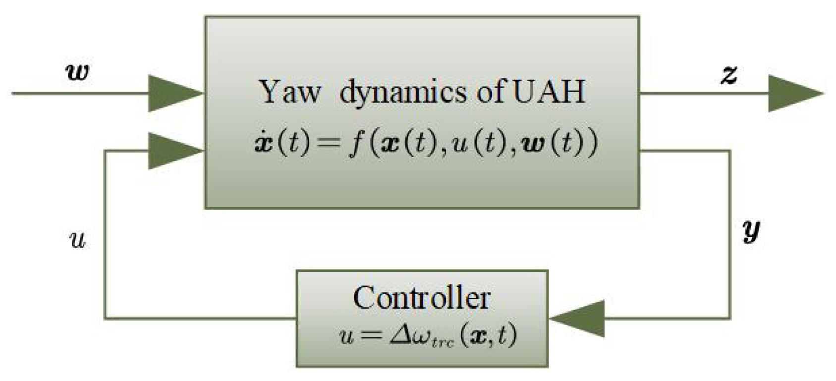
  • A fourth-order yaw error dynamic model considering actuator output fault, matched and unmatched disturbances is constructed. Based on the adaptive command filtered method, we built a simple control framework with no need for using DOB and solving complex HJI inequality to attenuate system multi-source perturbation.
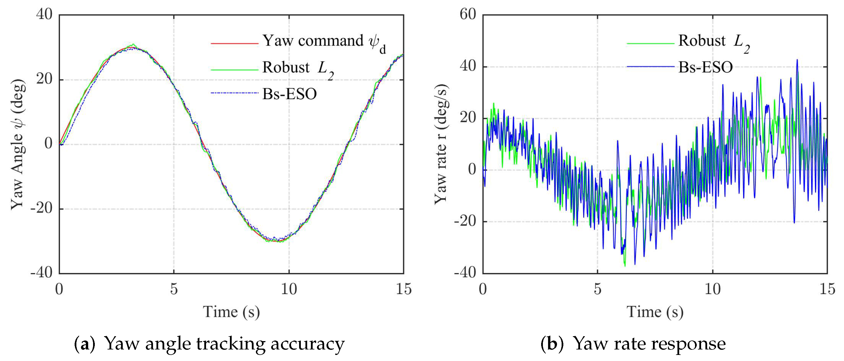
  • A rigorous stability analysis of the closed-loop yaw system was completed, which achieved the predefined performance of L 2 -gain disturbance suppression. Four groups of comparative simulation results show the effectiveness and superiority of this control law.
The rest is organized as follows: Section 2 introduces the fourth-order yaw error dynamic equation. Section 3 presents the definitions of system’s output performance evaluation and control law, then gives the proof based on analysis of Lyapunov stability. Section 4 verifies the proposed controller in the Xcell60 UAH simulation platform by comparing with the extended state observer-based backstepping method. Finally, the conclusions and future work are briefly described in Section 5.

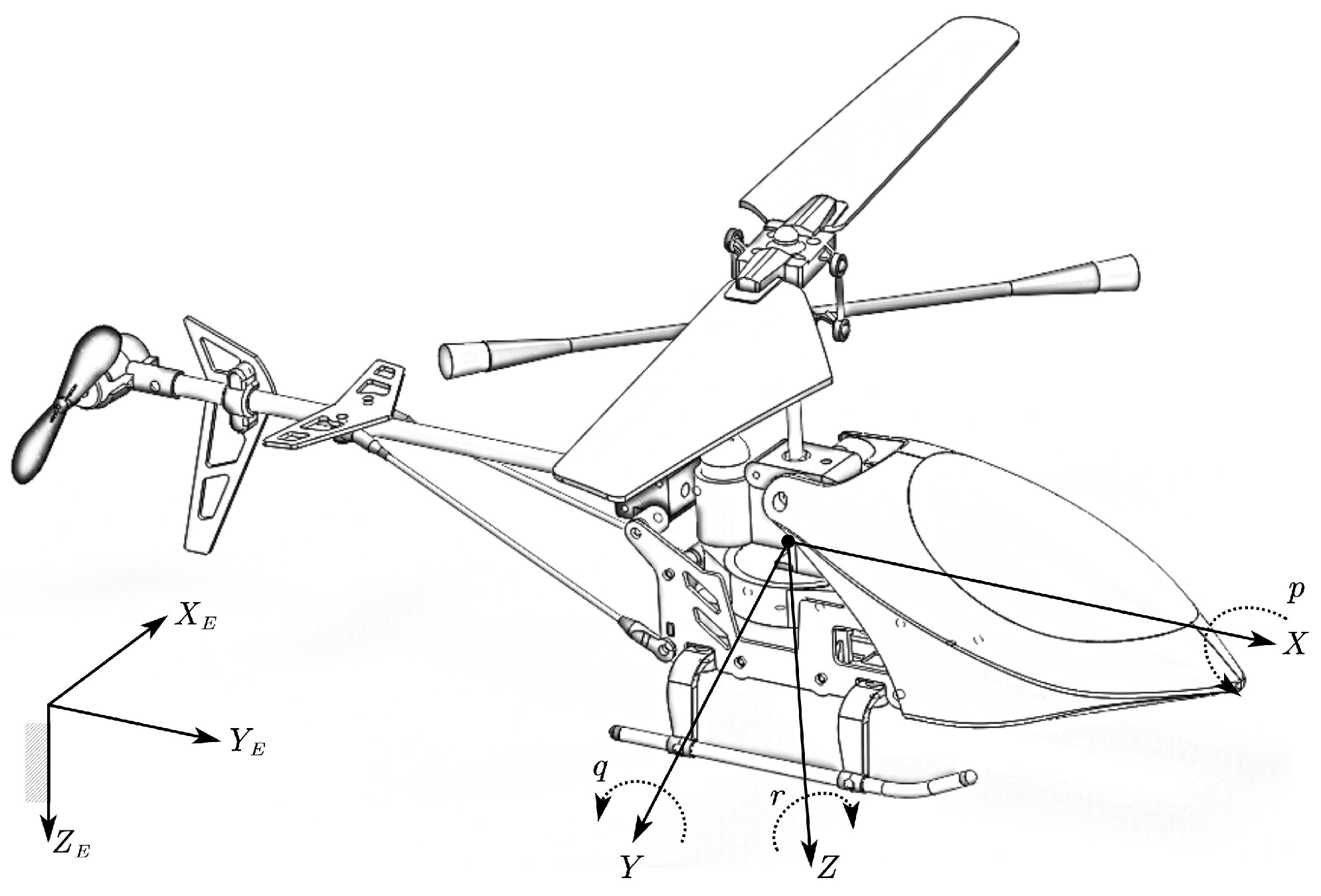
2. Yaw Error Dynamic Model

A small-scale unmanned aerial helicopter’s dynamics are described by the Newton–Euler modeling method. The ground and body coordinates are depicted in Figure 1, and its yaw motion equation is given as follows:
ψ ˙ ( t ) = sin ϕ ( t ) cos θ ( t ) q ( t ) + cos ϕ ( t ) cos θ ( t ) r ( t ) + w 1 ω b ( t ) , Ω ( t ) , t r ˙ ( t ) = I x x I y y I z z p ( t ) q ( t ) + N r r ( t ) + N c δ c o l ( t ) + T t r ω t r ( t ) , δ t r ( t ) + w 2 w wind ( t ) , t
where Ω = [ ϕ , θ , ψ ] T are the Euler attitude angles; ω b = [ p , q , r ] T are the angular rates in body coordinates, with roll, pitch and yaw, respectively. N r and N c are unknown aerodynamic parameters in an equilibrium state; I ( . ) represents rotational inertia to the corresponding axis; T t r is the aerodynamic force of tail rotor, which depends on its rotational speed and ω t r and pitch angle δ t r ; w 1 is mismatched disturbance, mainly resulting from noisy signals; w 2 denotes matched disturbance aroused by uncertain dynamics and external turbulent flow. Clearly, when p , q approaches zero without noise, ψ ˙ r . Consider that the helicopter is in the hover state without wind disturbance. The aerodynamic force of the tail rotor can be calculated offline by the standard blade element method and represented as
T t r ω t r , δ t r = p 0 + p 1 ω t r + p 2 δ t r + p 3 ω t r δ t r + p 4 δ t r 2 + p 5 ω t r 2
where p i is the constant parameter known by numerical calculation, ω t r is the rotating speed of the tail rotor and δ t r represents its pitch angle that is controlled by a servo device. For a constant pitch rotor, δ t r is deemed as constant. The force can be linearized as affine at trim point ( ω t r 0 , δ t r 0 )
T t r = T t r ( ω t r 0 , δ t r 0 ) + T t r ω t r Δ ω t r = T 0 + k w Δ ω t r
obviously, k w = p 1 + p 2 δ t r 0 + 2 p 5 ω t r 0 , Δ ω t r is the speed increment driven by a motor. Generally, the current regulation period is about 50∼200 μ s, much less than the speed control period of around 5∼20 ms, so the electrical dynamics of tail rotor system can be ignored. Thus, the mechanical dynamics are described as
τ Δ ω t r ˙ ( t ) = Δ ω t r ( t ) + ( 1 + Δ k ( t ) ) Δ ω t r c ( t ) + w ¯ 3 ( ω t r , t )
where τ denotes the time constant of system; Δ k ( t ) represents the motor fault; 1 < Δ k ( t ) k m and k m are unknown, w ¯ 3 ; and is the modeling error. To improve the tracking accuracy of yaw motion, we firstly define the yaw error e ψ = ψ ψ d , and thus obtain integrated error e I = t 0 t e ψ d t . Combining the equations of (1), (3) and (4), the yaw error dynamic model under multi-source disturbances is governed by
e ˙ I ( t ) = e ψ ( t ) e ˙ ψ ( t ) = ψ ˙ d ( t ) + s ϕ ( t ) c θ ( t ) q ( t ) + c ϕ ( t ) c θ ( t ) r ( t ) + w 1 ω b ( t ) , Ω ( t ) , t r ˙ ( t ) = T 0 + N r r ( t ) + I r p ( t ) q ( t ) + N c δ c o l ( t ) + k w Δ ω t r ( t ) + w 2 w wind ( t ) , t Δ ω ˙ t r ( t ) = 1 τ Δ ω t r ( t ) + 1 τ 1 + Δ k ( t ) Δ ω t r c ( t ) + w 3 ω t r ( t ) , t
where I r = ( I x x I y y ) / I z z ψ d ( t ) represents the desired yaw angular; s ( · ) , c ( · ) denote sine and cosine operators; the control input is u = Δ ω t r c ( t ) ; and unknown parameter vector W = [ N r , I r , N c ] T , w = [ w 1 , w 2 , w 3 ] is the disturbance source. We define x = [ e I , e ϕ , r , Δ ω t r ] T as the system’s state. It can be seen that the dynamics are a strict-feedback nonlinear system, which is suitable for a backstepping control strategy, but this method has the inherent problem of differential explosion for the high-order system. Thus, in the next section, the command filtered adaptive backstepping approach [24] will be introduced to acquire the derivations of virtual functions.
To facilitate the controller design and analysis, some preliminaries are stated as follows.
Lemma 1.
For any x , y R n , the following inequality holds:
x T y 1 2 γ 2 x T x + γ 2 2 y T y
Lemma 2
([25]). For given r 0 , any x , y R , the inequality | x + y | r c r | x | r + | y | r holds, where c r = 2 r 1 when r 0 ; c r = 1 , for 0 r < 1 .
Lemma 3
([26]). For x i R , i = 1 , 2 , . . . , n , 0 < p < 1 ,
i = 1 n x i p i = 1 n x i p n 1 p i = 1 n x i p
Assumption 1.
The desired yaw trajectory ψ d and its time derivative ψ d ˙ are known and bounded.
Assumption 2.
The pitch motion ( θ , q ) and roll ( ϕ , p ) of UAH have stabilized under the main rotor controller; all signals are bounded.

3. Controller Design

The nonlinear H control has excellent performance for a system with uncertainty and disturbance, which is associated with solving the complex Hamilton–Jacobi–Issacs (HJI) partial differential equality or inequality. This paper proposes a well-defined H yaw control scheme in the sense of a uniform-ultimately bounded and system L 2 -gain without the solution of the HJI equation, as shown in Figure 2. We firstly describe the multi-source disturbances attenuation problem of UHA’s yaw motion as follows.
Definition 1.
The yaw closed-loop system is called finitely L 2 -gain stable for a designed control law u = Δ ω t r c ( x , t ) if the following conditions hold:
(1)
When w = 0 , all signals are uniform-ultimately bounded stable.
(2)
When w 0 , the evaluation signal vector z for initial state x ( 0 ) = 0 , T > 0 satisfies
0 T z 2 d t γ 2 0 T w 2 d t + ε , w L 2 [ 0 , T ]
ε is a sufficiently small constant [27], the z = h ( x ) is a state-dependent vector and h ( x ) is designed later.
Based on the yaw error dynamic model (5), we define the tracking errors:
x ¯ 1 = x 1 , x ¯ i = x i x i c , i = 2 , 3 , 4
x i c is the output of the filter x ˙ i c = ω i ( x i c α i 1 ) , x i c ( 0 ) = α i 1 ( 0 ) , ω i > 0 is the time constant of the filter, α i represents the virtual control function in every step and α 0 = 0 . Clearly, there is a time ( T 1 i > 0 ) when the filter error | x i c ( T 1 i ) α i 1 ( T 1 i ) | < ϵ i will be small enough [24]. The virtual control law α i is designed as
α 1 = c 1 + k 1 2 2 v 1 k 11 ξ 1 μ 1 k 12 sign ( ξ 1 ) α 2 = c θ c ϕ ψ ˙ d c 2 + k 2 2 2 + 1 2 γ 2 v 2 k 21 ξ 2 μ 1 k 22 sign ( ξ 2 ) s ϕ c θ q x ¯ 1 + x ˙ 2 c α 3 = 1 k w T 0 Φ 1 T W ^ c 3 + k 3 2 2 + 1 2 γ 2 v 3 k 31 ξ 3 μ 1 k 32 sign ( ξ 3 ) c ϕ c θ x ¯ 2 + x ˙ 3 c
where c i > 0 , k i > 0 , k i i > 0 , i = 1 , 2 , 3 , 4 , γ is the given performance index of disturbance attenuation, μ 1 R p / q 1 , and R p / q 1 : = { p / q | p , q R odd + , p q } . Φ = r , p q , δ c o l T represents the known or measurable signals. W ^ is the estimated value of W = N r , I r , N c T . v = v 1 , v 2 , v 3 , v 4 T is the compensated error vector and defined as
v = x ¯ ξ
the compensated signal ξ = ξ 1 , ξ 2 , ξ 3 , ξ 4 T is designed to eliminate the effect of filtering error to the virtual control yaw, and it is designed as
ξ 1 ˙ = k 11 ξ 1 μ 1 k 12 sign ( ξ 1 ) + ξ 2 c α 1 + ξ 2 ξ 2 ˙ = k 21 ξ 2 μ 1 k 22 sign ( ξ 2 ) + c ϕ c θ ( x 3 c α 2 ) ξ 1 + c ϕ c θ ξ 3 ξ 3 ˙ = k 31 ξ 3 μ 1 k 32 sign ( ξ 3 ) + k w ( x 4 c α 3 ) c ϕ c θ ξ 2 + k w ξ 4 ξ 4 ˙ = k 41 ξ 4 μ 1 k 42 sign ( ξ 4 ) k w ξ 3
Define the evaluation function of system output
z = h ( x ) = K v
where K = diag ( k 1 , k 2 , k 3 , k 4 ) represents the penalty matrix. The smaller the evaluation function is, the closer the system’s state is to the ideal virtual control function. Thus, yaw error can be sufficiently small. The estimated law of aerodynamic parameters is designed as
W ^ ˙ = v 3 Γ Φ σ 1 Γ W ^
where the Γ is a symmetric positive matrix, σ 1 > 0 . Finally, the yaw control law is designed as
Δ ω t r c = τ 1 τ x 4 c 4 + k 4 2 2 + 1 2 γ 2 v 4 ρ ^ sign ( v 4 ) k 41 ξ 4 μ 1 k 42 sign ( ξ 4 ) k w x ¯ 3 + x ˙ 4 c
where the ρ = 1 τ k m | Δ W t r | max represents the maximum oscillation rate of rotor speed when some faults occur to the motor, and its estimated law is designed as
ρ ^ ˙ = k ρ | v 4 | k ρ σ 2 ρ ^
where k ρ > 0 , σ 2 > 0 , ρ ^ ( 0 ) > 0 . Based on the above analysis, the following theorem can be obtained:
Theorem 1.
Consider the yaw error dynamics (5) under multi-source disturbances. If the control law is given as (13) with virtual functions (9), parameters’ estimation laws (12) and (14) and the error compensation signal (11), then the yaw closed-loop system will achieve finite L 2 -gain that is stable as described in Definition 1.
Proof 
Selecting the following Lyapunov function,
V ¯ = 1 2 v T v
Taking the derivative of V along the yaw dynamics and control law,
V ¯ ˙ = i 4 v i ( x ˙ i x ˙ i c ξ ˙ i ) = v 1 ( x ¯ 2 + α 1 + x 2 c α 1 x ˙ 1 c ξ ˙ 1 ) + v 2 ψ ˙ d + s ϕ c θ q + c ϕ c θ ( x ¯ 3 + α 2 + x 3 c α 2 ) + w 1 x ˙ 2 c ξ ˙ 2 + v 3 T 0 + Φ T W + k w ( x ¯ 4 + α 3 + x 4 c α 3 ) + w 2 x ˙ 3 ξ ˙ 3 + v 4 1 τ Δ ω t r + 1 τ ( 1 + Δ k ( t ) ) Δ ω t r c + w 3 x ˙ 4 c ξ ˙ 4
Applying the virtual function’s (9), dynamics of the compensating signal in (11), control law (13) and parameter estimation law (12) and (14):
V ¯ ˙ v 1 c 1 + k 1 2 2 v 1 + v 2 + v 2 c 2 + k 2 2 2 + 1 2 γ 2 v 2 v 1 + c ϕ c θ v 3 + w 1 + v 3 c 3 + k 3 2 2 + 1 2 γ 2 v 3 c ϕ c θ v 2 + k w v 4 Φ 1 T W ˜ + w 2 + v 4 c 4 + k 4 2 2 + 1 2 γ 2 v 4 ρ ^ sign ( v 4 ) k w v 3 + w 3 + ρ | v 4 | i = 1 4 c i + k i 2 2 v i 2 1 2 γ 2 i = 2 4 v i 2 v 3 Φ T W ˜ + i = 1 3 v i + 1 w i ρ ˜ | v 4 |
Define the Lyapunov function:
V ( v , W ˜ , ρ ˜ ) = V ¯ + 1 2 W ˜ T Γ 1 W ˜ + 1 2 k ρ ρ ˜ 2
Then comes derivative V, along with the adaptive laws (12) and (14):
V ˙ ( v , W ˜ , ρ ˜ ) = V ¯ ˙ + W ˜ T Γ 1 W ^ ˙ + k ρ 1 ρ ˜ ρ ^ ˙ = V ¯ ˙ + W ˜ Γ 1 v 3 Γ Φ σ 1 Γ W ^ + ρ ˜ k ρ 1 k ρ | v 4 | k ρ σ 2 ρ ^ i = 1 4 c i + k i 2 2 v i 2 1 2 γ 2 i = 2 4 v i 2 + i = 1 3 v i + 1 w i σ 1 W ˜ T W ^ σ 2 ρ ˜ ρ ^
Define H = V ˙ + 1 2 z γ 2 w 2 ; then,
H i = 1 4 c i v i 2 1 2 γ 2 i = 2 4 v i 2 + i = 1 3 v i + 1 w i γ 2 2 w 2 σ 1 W ˜ T W ^ σ 2 ρ ˜ ρ ^ i = 1 4 c i v i 2 1 2 γ 2 i = 2 4 v i 2 + 1 2 γ 2 i = 1 3 v i + 1 2 + γ 2 2 i = 1 3 w i 2 γ 2 2 w 2 σ 1 W ˜ T W ^ σ 2 ρ ˜ ρ ^ i = 1 4 c i v i 2 σ 1 2 W ˜ 2 + σ 1 2 W 2 σ 2 2 | ρ ˜ | 2 + σ 2 2 | ρ | 2 α · 1 2 i = 1 4 v i 2 σ 1 λ max ( Γ 1 ) · 1 2 W ˜ Γ 1 W ˜ k ρ σ 2 1 2 k ρ ρ ˜ 2 + σ 1 2 W 2 + σ 2 2 | ρ | 2 = a V + η
where α = min 2 c i , a = min { α , σ 1 / λ max ( Γ 1 ) , σ 2 k ρ } , λ max represents the maximum eigenvalue, η = ( σ 1 W 2 + σ 2 | ρ | 2 ) / 2 , so
V ˙ + a V 1 2 γ 2 w 2 z 2 + η
When w = 0 , obviously, V ˙ + a V ˙ η . Thus, there exists a compact set Ω ( v , W ˜ , ρ ˜ ) , and V ˙ 0 once system trajectory enters the outside of the compact set, so system signals v , W ˜ , ρ ˜ will be uniform-ultimately bounded (UUB). The system state tracking error is x ¯ = v + ξ , if the ξ is convergent, then x ¯ will also be UUB. Next, it is verified that ξ has fast finite-time stability. Define the following function and derivative it:
V ξ = 1 2 i = 1 4 ξ i 2
V ˙ ξ = ξ 1 k 11 ξ 1 μ 1 k 12 sign ( ξ 1 ) + x 2 c α 1 + ξ 2 + ξ 2 k 21 ξ 2 μ 1 k 22 sign ( ξ 2 ) + c ϕ c θ x 3 c α 2 ξ 1 + c ϕ c θ ξ 3 + ξ 3 k 31 ξ 3 μ 1 k 32 sign ( ξ 4 ) + k w ( x 4 c α 3 ) c ϕ c θ ξ 2 + k w ξ 4 + ξ 4 k 41 ξ 4 μ 1 k 42 sign ( ξ 4 ) k w ξ 3 = i = 1 4 k i 1 ξ i μ 1 + 1 i = 1 4 k i 2 | ξ i | + ξ 1 x 2 c α 1 + ξ 2 c ϕ c θ x 3 c α 2 + ξ 3 k w ( x 4 c α 3 ) k i 1 , m i = 1 4 1 2 ξ i 2 ( μ 1 + 1 ) / 2 i = 1 4 k i 2 | ξ i | + ρ i = 1 3 | ξ i | | x i + 1 c α i | k i 1 , m 2 μ 1 1 V ξ ( μ 1 + 1 ) / 2 2 k i 2 , m V ξ 1 / 2 + 2 ρ ϖ V ξ 1 / 2 ϱ 1 V ξ β 2 ( k i 2 , m ρ ϖ ) V ξ 1 / 2
where Lemmas 2 and 3 are used for the above inequality. k i 1 , m = min k i 1 , k i 2 , m = min k i 2 , ϖ = max { ϖ i } , ρ = max { 1 , c ϕ / c θ , k w } , β = ( μ 1 + 1 ) / 2 , ϱ 1 = k i 1 , m 2 μ 1 1 , μ 1 R p / q 1 . Define ϱ 2 = 2 ( k i 2 , m ρ ϖ ) > 0 ; thus, the inequality can be written as
V ˙ ξ + ϱ 1 V ξ β 1 + ϱ 2 V ξ 1 / 2 0
Based on Theorem 1 in [25], the compensated signal ξ will be finite-time stable when t > T ξ , ξ = 0 , where
T ξ = max T 1 i + 2 ϱ 2 + V ξ 1 β ( 0 ) 1 ϱ 1 ( 1 β )
so state tracking error x ¯ will be UUB, and Equation (9) and Assumption 2 imply the virtual control law α i is also UUB. Thus system, state x is UUB when w = 0 . Namely, all signals are uniformly ultimately bounded stable, satisfying condition (1) in Definition 1.
When w 0 , inequality (17) implies
V ˙ 1 2 γ 2 W 2 z 2 + η
Integrate both sides of this inequality at zero initial condition, and choose σ i = e β t , yielding
0 T z 2 d t γ 2 0 T w 2 d t + W 2 + | ρ | 2 2 o T e β t d t , w L 2 ( 0 , T )
That is, condition (2) in Definition 1 is satisfied.
To sum up the above analysis, this section has completed the design of a nonlinear robust yaw control scheme for a small UAH with a pure variable-speed tail rotor. The yaw closed-loop system can be adjusted to resist multiple disturbance sources by presetting disturbance suppression performance index γ . It is noteworthy that a pretty small value γ will lead to a relatively large control energy; a compromise between the two is needed in practice. The proposed controller is verified in the next section.

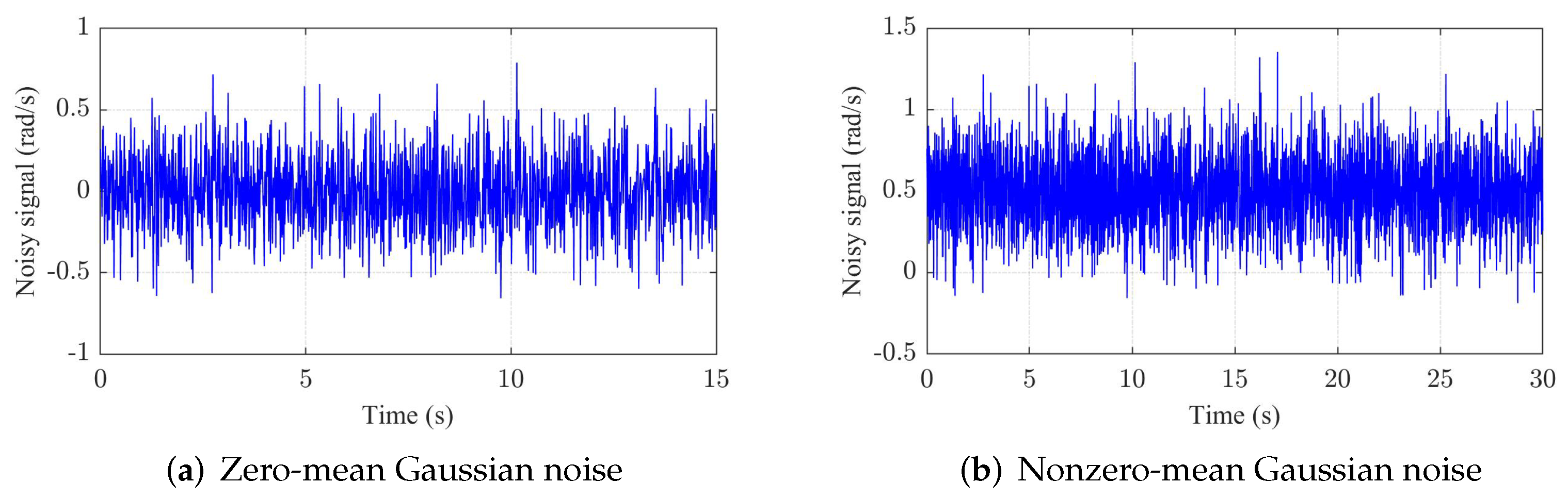
4. Simulation Results

The proposed yaw controller was tested in the Xcell60 unmanned helicopter simulation platform, not just in a pure yaw dynamic model. Four groups of simulation experiments were performed to show the disturbance suppression ability of the prototype against noisy signals, motor faults, internal parameter perturbation and outside airflow turbulence in hovering and cruising flight states. In order to illustrate the advantages and disadvantages of the proposed robust L 2 disturbance attenuation approach, comparisons are carried out with a nonlinear backstepping controller and an extended state observer (Bs-ESO) proposed by Zhao et al. [11]. The main rotor was dominated by a linear controller. The pitch angle of the tail rotor had a trim value of 0.0227 rad, and baseline blade speed was 787.54 rad/s. Parameters of the rotor’s force model were: k w = 0.2318 , T 0 = 9.2642 . The robust L 2 controller parameters were designed as c = [ 1 , 2 , 2 , 2 ] , k = [ 1 , 2 , 2 , 2 ] , k i 1 = [ 5 , 5 , 5 , 5 ] , k i 2 = [ 1 , 1 , 1 , 1 ] , γ = 0.5 , σ 1 = σ 2 = e 2 t , ω 2 = 15 , ω 3 = 25 , ω 4 = 40 , τ = 0.01 , μ 1 = 1 , Γ = diag ( 5 , 5 , 5 ) , k ρ = 5 . The Bs-ESO control law was designed as
Δ ω t r = 1 k w ( N r r I r p q T 0 d ^ cos ϕ cos θ e ψ + r c ˙ k 2 ( r r c ) )
where r c = cos θ ( k 1 e ψ ψ d ˙ + sin ϕ q / cos θ ) / cos ϕ , k 1 = 10 , k 2 = 15 . d ^ is the estimated value of lumped disturbance in the yaw channel by ESO; the observer gain is L = [ 15 , 10 ] .
In the first group of simulations, the performance of the proposed controller in resisting mismatched noise disturbance was investigated. The prototype was in a hovering state. Random Gaussian noises with variance of 0.05, with zero and nonzero means, were injected to the feedback attitude rate signal, p , q and r, respectively, which are shown in Figure 3.
The yaw motion tracking and stabilizing performance are compared in Figure 4 and Figure 5, considering the situation that angular rate sensor is accompanied by zero-mean noise disturbance. The command was set as ψ d = 30 sin ( 0.5 t ) deg. It can be easily seen that robust L 2 and Bs-ESO have similar dynamic capabilities and steady-state precision. The tracking performance of the proposed method is slightly better than that of Bs-ESO, but for the stabilizing, the opposite.
Furthermore, Figure 6 shows the results in face of nonzero-mean noise environment. Obviously, the yaw angle of Bs-ESO deviates from the expected value; by contrast, the tracking error of the robust L 2 approach was small.
The second group of simulations verified the ability to resist motor fault disturbance. The deviation of the driven motor’s response to step instructions kept in Δ k = 0.3 sin ( t ) . Responses to the sine command are shown in Figure 7. It can be seen that two controllers achieved similar tracking accuracy, but the yaw rate oscillation of the proposed robust L 2 is lower in comparison with that of Bs-ESO. Likewise, Figure 8 depicts the linear tracking ability in the presence of a motor harmonic fault. The two methods showed similar performance after a short transient period.
Additionally, Figure 9 further studies the yaw channel’s ability to suppress large-scale internal disturbances, considering both nonzero-mean random noise and motor fault perturbation. Results show that the proposed approach has higher accuracy after the initial stage, but Bs-ESO has static error.
Subsequently, the simulations verified the effect of the compensation term in the control law, as shown in Figure 10. The angle responses of controllers with and without compensation are compared. It can be seen that in the initial stage, the output angles of two modes were basically the same because closed-loop system did not enter the stable state. However, after entering the steady state, the closed-loop system with compensation greatly improved the stabilizing accuracy, and the fluctuation caused by motor fault was suppressed.
The third group of simulations tested the controller’s resistance to external airflow disturbance during cruising. Wind in body coordinates are shown in Figure 11, which were produced by the Dryden turbulence model. The helicopter prototype gradually accelerated its flight speed to about 10 m/s. The results are shown in Figure 12. The two controllers showed nearly steady state accuracy. Their amplitudes and yaw rate were also about 10 deg/s, which is still within an allowable range.
Finally, Figure 13 illustrates the robustness of the proposed control law to model parameters. According to Equation (13), the yaw law design only needs rotor parameters of k w and T 0 . It can be seen from the figure that although parameter k w is enlarged and reduced by two times, the yaw steady-state accuracy remains basically unchanged. Only a slight oscillation occurs in the initial stage.
Figure 14 shows stabilizing performance for different disturbance attenuation indexes γ in the proposed control law. It indicates a smaller γ value will improve the dynamic accuracy. The yaw error is smaller than for a larger index. For instance, when γ = 1 , the angle error in whole stage is too large, and the corresponding yaw rate has exceeded the allowable range; in this case γ = 0.3 is an appropriate value. Therefore, it is easy to enhance the performance of attenuating the multi-source disturbances by adjusting the γ value in the control law.
As a result, we can conclude that the proposed robust L 2 controller has the advantages of coping with nonzero-mean noise and motor output faults. It maintains higher tracking and stabilizing accuracy compared with the Bs-ESO controller. The performances of these two methods are close under zero-mean noise environment or external airflow perturbation.

5. Conclusions

In this article, a nonlinear robust control scheme is proposed to deal with multi-source disturbances in the sense of UUB and finite system L 2 -gain for a small UAH yaw channel operated in pure variable-speed mode. Firstly, a fourth-order yaw error dynamics model is established, considering sensor signals noise, actuator fault and external load fluctuation; and then according to the predetermined performance index, an adaptive filtered command yaw controller consisting of the laws of virtual functions, parameters estimation and compensation signal is designed. Subsequently, stability analysis shows the closed-loop system is able to achieve the predefined capability to disturbance attenuation. Finally, the effectiveness of proposed method is verified with the Xcell60 UHA prototype platform by comparing it with the backstepping controller together with an extended state observer. Results show that the yaw closed-loop system can meet the requirements of resistance to mismatched noise disturbance, motor failure, external airflow and model parameter error by selecting an appropriate index γ . A smaller value of γ implies excessive control energy, probably resulting in a large output oscillation; therefore, a direct computing method for an optimal performance index will be explored in future work.

Author Contributions

Conceptualization, P.T. and Y.D.; methodology, P.T.; software, J.C.; validation, P.T. and Y.D.; formal analysis, P.T.; investigation, P.T.; resources, Y.D. and J.C.; data curation, J.C.; writing—original draft preparation, P.T.; writing—review and editing, Y.D.; visualization, P.T.; supervision, Y.D.; project administration, Y.D.; funding acquisition, Y.D. All authors have read and agreed to the published version of the manuscript.

Funding

This research was funded by the Science and Technology Department of Sichuan Province, grant number: 2020YFS0004.

Institutional Review Board Statement

Not applicable.

Informed Consent Statement

Not applicable.

Data Availability Statement

Data is contained within the article.

Conflicts of Interest

The authors declare no conflict of interest.

Abbreviations

The following abbreviations are used in this manuscript:
UAHUnmanned Aerial Helicopter
AYDSArtificial Yaw Damping System
ADRCActive Disturbance Rejection Control
SMCSliding Mode Control
DOBDisturbance-Observer-Based
UUBUniform-Ultimately bounded
HJIHamilton–Jacobi-Issacs
BsBackstepping
ESOExtended State Observer
RBFRadial Basis Function

References

  1. La Civita, M.; Papaueorgiou, G.; Messner, W.C.; Kanade, T. Design and flight testing of an H(infinity) controller for a robotic helicopter. J. Guid. Control Dyn. 2006, 29, 485–494. [Google Scholar] [CrossRef]
  2. Nedjati, A.; Vizvari, B.; Izbirak, G. Post-earthquake response by small UAV helicopters. Nat. Hazards 2016, 80, 1669–1688. [Google Scholar] [CrossRef]
  3. Ding, L.; Ma, R.; Wu, H.; Feng, C.; Li, Q. Yaw control of an unmanned aerial vehicle helicopter using linear active disturbance rejection control. Proc. Inst. Mech. Eng. Part I-J. Syst. Control Eng. 2017, 231, 427–435. [Google Scholar] [CrossRef]
  4. Ding, L.; He, Q.; Wang, C.; Qi, R. Disturbance Rejection Attitude Control for a Quadrotor: Theory and Experiment. Int. J. Aerosp. Eng. 2021, 2021, 8850071. [Google Scholar] [CrossRef]
  5. Xu, D.Z.; Jiang, B.; Shi, P. Global Robust Tracking Control of Non-affine Nonlinear Systems with Application to Yaw Control of UAV Helicopter. Int. J. Control Autom. Syst. 2013, 11, 957–965. [Google Scholar] [CrossRef]
  6. Jiang, T.; Lin, D.; Song, T. Novel integral sliding mode control for small-scale unmanned helicopters. J. Frankl. Inst. 2019, 356, 2668–2689. [Google Scholar] [CrossRef]
  7. Krishna, A.B.; Sen, A.; Kothari, M. Super Twisting Algorithm for Robust Geometric Control of a Helicopter. J. Intell. Robot. Syst. Theory Appl. 2021, 102, 61. [Google Scholar] [CrossRef]
  8. Ullah, I.; Pei, H.L. Fixed Time Disturbance Observer Based Sliding Mode Control for a Miniature Unmanned Helicopter Hover Operations in Presence of External Disturbances. IEEE Access 2020, 8, 73173–73181. [Google Scholar] [CrossRef]
  9. Liu, L.; Chen, M.; Li, T.; Wang, H. Composite Anti-Disturbance Reference Model L2L Control for Helicopter Slung Load System. J. Intell. Robot. Syst. Theory Appl. 2021, 102, 15. [Google Scholar] [CrossRef]
  10. Tang, S.; Mao, L.; Liu, G.; Wang, W. Active Disturbance Rejection Control Design of the Yaw Channel for a Small-scale Helicopter based on Backstepping. In Proceedings of the 38th 2019 Chinese Control Conference (CCC), Guangzhou, China, 27–30 July 2019; pp. 8073–8078. [Google Scholar]
  11. Zhao, W.; Meng, Z.; Wang, K.; Zhang, H. Backstepping Control of an Unmanned Helicopter Subjected to External Disturbance and Model Uncertainty. Appl. Sci. 2021, 11, 5331. [Google Scholar] [CrossRef]
  12. Chen, X.; Zhang, Q.; Duan, Y. Finite-Time Backstepping Sliding Mode Control Applied to the Yaw Control of UAV Helicopters with Actuator Faults. In Proceedings of the 39th Chinese Control Conference, Shenyang, China, 27–29 July 2020; pp. 6911–6916. [Google Scholar] [CrossRef]
  13. Li, Y.; Chen, M.; Ge, S.S. Anti-disturbance control for attitude and altitude systems of the helicopter under random disturbances. Aerosp. Sci. Technol. 2020, 96, 105561. [Google Scholar] [CrossRef]
  14. Sheng, S.; Sun, C. Yaw Control of an Unmanned Helicopter Using Adaptive Model Feedback and Error Compensation. J. Aerosp. Eng. 2016, 29, 06015002. [Google Scholar] [CrossRef]
  15. Soltanpour, M.R.; Hasanvand, F.; Hooshmand, R. Robust linear parameter varying attitude control of a quadrotor unmanned aerial vehicle with state constraints and input saturation subject to wind disturbance. Trans. Inst. Meas. Control 2020, 42, 1083–1096. [Google Scholar] [CrossRef]
  16. Fan, X.; Yi, Y.; Zhang, T. Disturbance rejection control of yaw channel of a small-scale unmanned helicopter via Takagi-Sugeno disturbance modeling approach. Int. J. Adv. Robot. Syst. 2016, 13, 1729881416671113. [Google Scholar] [CrossRef]
  17. Yan, W.X.; Huang, J.; Xu, D.Z. Adaptive fuzzy tracking control for non-affine nonlinear yaw channel of unmanned aerial vehicle helicopter. Int. J. Adv. Robot. Syst. 2017, 14, 1729881416678137. [Google Scholar] [CrossRef] [Green Version]
  18. Le, T.Q.; Lai, Y.C.; Yeh, C.L. Adaptive tracking control based on neural approximation for the yaw motion of a small-scale unmanned helicopter. Int. J. Adv. Robot. Syst. 2019, 16, 1729881419828277. [Google Scholar] [CrossRef] [Green Version]
  19. Lai, Y.C.; Le, T.Q. Adaptive Learning-Based Observer With Dynamic Inversion for the Autonomous Flight of an Unmanned Helicopter. IEEE Trans. Aerosp. Electron. Syst. 2021, 57, 1803–1814. [Google Scholar] [CrossRef]
  20. Shen, S.; Xu, J. Adaptive neural network-based active disturbance rejection flight control of an unmanned helicopter. Aerosp. Sci. Technol. 2021, 119, 107062. [Google Scholar] [CrossRef]
  21. Zhang, Q.; Chen, X.; Xu, D. Adaptive Neural Fault-Tolerant Control for the Yaw Control of UAV Helicopters with Input Saturation and Full-State Constraints. Appl. Sci. 2020, 10, 1404. [Google Scholar] [CrossRef] [Green Version]
  22. Ezekiel, D.M.; Samikannu, R.; Matsebe, O. Pitch and Yaw Angular Motions (Rotations) Control of the 1-DOF and 2-DOF TRMS: A Survey. Arch. Comput. Methods Eng. 2021, 28, 1449–1458. [Google Scholar] [CrossRef]
  23. Singh, R.; Bhushan, B. Data-Driven Technique-Based Fault-Tolerant Control for Pitch and Yaw Motion in Unmanned Helicopters. IEEE Trans. Instrum. Meas. 2021, 70, 3502711. [Google Scholar] [CrossRef]
  24. Dong, W.; Farrell, J.A.; Polycarpou, M.M.; Djapic, V.; Sharma, M. Command filtered adaptive backstepping. IEEE Trans. Control Syst. Technol. 2011, 20, 566–580. [Google Scholar] [CrossRef]
  25. Sun, Z.Y.; Yun, M.M.; Li, T. A new approach to fast global finite-time stabilization of high-order nonlinear system. Automatica 2017, 81, 455–463. [Google Scholar] [CrossRef]
  26. Yu, J.; Shi, P.; Zhao, L. Finite-time command filtered backstepping control for a class of nonlinear systems. Automatica 2018, 92, 173–180. [Google Scholar] [CrossRef]
  27. Ishii, C.; Shen, T.; Qu, Z. Lyapunov recursive design of robust adaptive tracking control with L2-gain performance for electrically-driven robot manipulators. Int. J. Control 2001, 74, 811–828. [Google Scholar] [CrossRef]
Figure 1. Small-scale unmanned aerial helicopter with a variable-speed tail rotor.
Aerospace 09 00042 g001
Figure 2. A nonlinear robust yaw controller scheme.
Aerospace 09 00042 g002
Figure 3. Noisy signal of injecting to attitude rate.
Aerospace 09 00042 g003
Figure 4. Yaw tracking performance under zero-mean noise disturbance.
Aerospace 09 00042 g004
Figure 5. Yaw stabilizing performance under zero-mean noise disturbance.
Aerospace 09 00042 g005
Figure 6. Yaw tracking and stabilizing under nonzero-mean noise disturbance.
Aerospace 09 00042 g006
Figure 7. Sine tracking performance in the presence of a harmonic motor fault.
Aerospace 09 00042 g007
Figure 8. Linear tracking performance in the presence of a harmonic motor fault.
Aerospace 09 00042 g008
Figure 9. Performance at suppressing the internal disturbances.
Aerospace 09 00042 g009
Figure 10. Effectiveness of the compensation term coping with motor faults.
Aerospace 09 00042 g010
Figure 11. Airflow speed in body coordinates.
Aerospace 09 00042 g011
Figure 12. Yaw stability performance under wind turbulence.
Aerospace 09 00042 g012
Figure 13. Steady-state accuracy for different model parameter.
Aerospace 09 00042 g013
Figure 14. Performance of disturbance attenuation index γ .
Aerospace 09 00042 g014
Publisher’s Note: MDPI stays neutral with regard to jurisdictional claims in published maps and institutional affiliations.

