Real-Time Precise Orbit Determination for LEO between Kinematic and Reduced-Dynamic with Ambiguity Resolution

Abstract

The real-time integer-ambiguity resolution of the carrier-phase observation is one of the most effective approaches to enhance the accuracy of real-time precise point positioning (PPP), kinematic precise orbit determination (KPOD), and reduced-dynamic precise orbit determination (RPOD) for low earth orbit (LEO) satellites. In this study, the integer phase clock (IPC) and wide-lane satellite bias (WSB) products from CNES (Centre National d’Etudes Spatiales) are used to fix ambiguity in real time. Meanwhile, the three models of real-time PPP, KPOD, and RPOD are applied to validate the contribution of ambiguity resolution. Experimental results show that (1) the average positioning accuracy of IGS stations for ambiguity-fixed solutions is improved from about 7.14 to 5.91 cm, with an improvement of around 17% compared to the real-time float PPP solutions, with enhancement in the east-west direction particularly significant, with an improvement of about 29%; (2) the average accuracy of the estimated LEO orbit with ambiguity-fixed solutions in the real-time KPOD and RPOD mode is improved by about 16% and 10%, respectively, with respect to the corresponding mode with the ambiguity-float solutions; (3) the performance of real-time LEO RPOD is better than that of the corresponding KPOD, regardless of fixed- or float-ambiguity solutions. Moreover, the average ambiguity-fixed ratio can reach more than 90% in real-time PPP, KPOD, and RPOD.

1. Introduction

The applications of low earth orbit (LEO) satellite data are successfully and widely demonstrated in various areas, such as remote sensing [1,2], communications [3,4], atmospheric sounding [5,6], radio occultation [7,8], ocean altimetry [9,10], and so on. The smooth realization of the above scientific tasks is inseparable from the precise orbit determination (POD) of LEO. To meet the growing needs for real-time spaceborne missions, such as LEO-enhanced real-time location service [11] and real-time atmospheric sounding [12], it is necessary to obtain precise orbits of LEO satellites in real time.

Since 2007, users have been able to apply the real-time pilot project (RTPP) provided by the International GNSS Service (IGS) to obtain the state-space representation (SSR) products of global navigation satellite systems (GNSS) satellites in real-time [13]. Meanwhile, with the support of the rapid development of GNSS onboard-receiver technology, real-time LEO POD can also be achieved. For instance, in the comparison of the real-time POD for GRACE (gravity recovery and climate experiment) series satellites between kinematic and reduced-dynamic modes, the accuracy for the GRACE-A/B satellite real-time POD based on the CLK93 orbit and the clock from CNES (Centre national d’etudes spatiales) can reach the sub-decimeter level [14]. Real-time GNSS satellite SSR corrections in some commercial companies, such as Fugro G4, are broadcasted by geostationary earth orbit (GEO) satellites. It is reported that 7 cm-accuracy kinematic LEO POD can be obtained in real-time mode from the Fugro G4 SSR products based on Swarm-C onboard observations [15]. In addition, the BeiDou navigation satellite system (BDS-3) precise point positioning (PPP) service of China [16,17], the new generation of the Australian/New Zealand (AU/NZ) satellite-based augmentation systems (SBAS)-aided PPP service [18], the Quasi-Zenith Satellite System (QZSS) of Japan [18,19], and Galileo’s high-precision PPP service in Europe [20] have their own way to provide real-time GNSS orbit and clock products for users. It is expected that the abovementioned real-time high-precision services will assist spaceborne missions that need precise orbital information.

LEO POD can be used mainly in two approaches, which are the reduced-dynamic method [21,22] and the kinematic method [22]. In theory, reduced-dynamic precise orbit determination (RPOD) and kinematic precise orbit determination (KPOD) for LEO basically have the same accuracy level [23]. However, affected by the noise of observations, poor geometric conditions, and short-term observation interruption, the performance of the KPOD mode is worse than that of the RPOD mode in practice [22]. Generally, orbital dynamic models and empirical accelerations can be introduced to improve the accuracy of LEO POD in the RPOD method [14]; however, the accuracy can also be further enhanced by correctly fixing the ambiguities of the carrier phase using the prior uncalibrated phase delays (UPD) or hardware-delay-offset (HDB) corrections in the satellites and receivers [24]. If float ambiguities can be successfully fixed as integers, the accuracy of LEO POD will be further improved [24]. There are mainly two methods for recovering integer ambiguities, which are double-difference (DD) [22,25] and single-receiver carrier phase integer-ambiguity resolution (IAR). The method of DD, by forming double-difference observation, can eliminate the common HDB between receivers and satellites in different paths. Single-receiver carrier phase IAR is an approach that applies externally calibrated products, such as UPD [26] or integer phase clock (IPC) products [27,28], to separate the ambiguities and HDB. The School of Geodesy and Geomatics at Wuhan University used the real-time UPD products calculated by themselves and performed real-time KPOD for Swarm-A and Sentinel-3A. Compared with the float solutions, the 3D-RMS (three-dimensional root mean square) has been improved by 16% and 27% for Swarm-A and Sentinel-3A, respectively [23]. Moreover, the CNES provided the wide-lane satellite bias (WSB) and dedicated IPC products for GPS (global positioning system) from 2009 [29] and Galileo since 2018 [30]. A study used the IPC products to fix ambiguities for post-processed POD for Swarm series satellites and found orbit accuracy can be improved by around 30–50% [31].

With the real-time demand of more and more spaceborne scientific missions, there are few articles giving points on the real-time onboard ambiguity resolution for LEO reduced-dynamic orbit determination or comparisons between real-time KPOD ambiguity resolution and RPOD ambiguity resolution. This work focuses on strengthening the observation model by real-time onboard ambiguity resolution to improve the performance of real-time LEO RPOD and KPOD in the future. We discuss the methodology of single-receiver carrier phase IAR-based IPC products in Section 2. Then, the real-time PPP and LEO POD strategies are presented in Section 3. In Section 4, the performances of real-time PPP, LEO KPOD, and LEO RPOD are validated against the proposed method, respectively. Conclusions of this work are finally presented in Section 5.

2. Methodology of Ambiguity Resolution

2.1. Observation Model

The zero-difference ambiguity-fixed method observation equations are given below for ground or LEO spaceborne receivers’ pseudo-range and carrier-phase measurements for double frequencies [14,32,33]:

$$\begin{array}{l}{P}_{r/LEO}^{s,f}={\rho }_{r/LEO}^s+c\left(\delta t_{r/LEO}-\delta t^s\right)+I_{r/LEO}^{s,f}+T_r^s+B_{r/LEO,P}^f-B_P^{s,f}+{\epsilon }_{r/LEO,P}^{s,f}\\ {\Phi }_{r/LEO}^{s,f}={\rho }_{r/LEO}^s+c\left(\delta t_{r/LEO}-\delta t^s\right)-I_{r/LEO}^{s,f}+T_r^s+B_{r/LEO,\Phi }^f-B_{\Phi }^{s,f}+N_{r/LEO}^{s,f}{\lambda }^f+{\epsilon }_{r/LEO,\Phi }^{s,f}\end{array}$$

(1)

where $s$ and $f$ represent GNSS satellite and carrier frequency, respectively; and subscript $r$ and $LEO$ refer to ground receivers and LEO spaceborne receivers, respectively. Other terms in Equation (1) can be expressed as follows:

• $P_{r/LEO}^{s,f}$, ${\Phi }_{r/LEO}^{s,f}$: pseudo-range and carrier-phase observation (m).
• ${\rho }_{r/LEO}^s$: geometric distance between ground receivers/LEO spaceborne receivers and GNSS satellites s antenna centers (m).
• $c$: speed of light (m/s).
• $\delta t_{r/LEO}$: ground receivers/LEO spaceborne receivers clock offsets (s).
• $\delta t^s$: GNSS satellites clock offsets (s).
• $I_{r/LEO}^{s,f}$: ionospheric delay (m).
• $T_r^s$: tropospheric delay (m). (LEO does not include tropospheric delay; Ground users include tropospheric delay).
• $B_{r/LEO,P}^f$, $B_P^{s,f}$: pseudo-range hardware delay biases of ground receivers/LEO spaceborne receivers and GNSS satellites (m).
• $B_{r/LEO,\Phi }^f$, $B_P^{s,f}$: carrier-phase hardware delay biases of ground receivers/LEO spaceborne receivers and GNSS satellites (m).
• ${\lambda }^f$: signal wavelength of frequency f (m).
• $N_{r/LEO}^{s,f}$: carrier-phase integer ambiguities (cycles).
• ${\epsilon }_{r/LEO,P}^{s,f}$, ${\epsilon }_{r/LEO,\Phi }^{s,f}$: multipath effects (m) and unmodeled pseudo-range and carrier-phase errors (m).

The ionosphere-free linear combination is the most widely used measurement model, which is applied to eliminate the first-order ionospheric delay [14,34,35,36,37]. Thus, it is used in the data processing of PPP and LEO POD in this study.

$$\begin{array}{l}{P}_{r/LEO,IF}^s=\frac{f_1^2}{f_1^2-f_2^2}{P}_{r/LEO}^{s,1}-\frac{f_2^2}{f_1^2-f_2^2}{P}_{r/LEO}^{s,2}\\ {\Phi }_{r/LEO,IF}^s=\frac{f_1^2}{f_1^2-f_2^2}{\Phi }_{r/LEO}^{s,1}-\frac{f_2^2}{f_1^2-f_2^2}{\Phi }_{r/LEO}^{s,2}\end{array}$$

(2)

Equations (1) and (2) are combined to obtain the expressions of the ionosphere-free measurement models that are listed hereafter [14,35,38,39].

$$\begin{array}{l}{P}_{r/LEO,IF}^s={\rho }_{r/LEO}^s+c\left(\delta t_{r/LEO}-\delta t^s\right)+T_r^s+B_{r/LEO,P}^{IF}-B_P^{s,IF}+{\epsilon }_{r/LEO,P_{IF}}^s\\ {\Phi }_{r/LEO,IF}^s={\rho }_{r/LEO}^s+c\left(\delta t_{r/LEO}-\delta t^s\right)+T_r^s+B_{r/LEO,\Phi }^{IF}-B_{\Phi }^{s,IF}+N_{r/LEO,IF}^s{\lambda }_{IF}+{\epsilon }_{r/LEO,{\Phi }_{IF}}^s\end{array}$$

(3)

where, $B_{r/LEO,P}^{IF}$ and $B_{r/LEO,\Phi }^{IF}$ indicate ionosphere-free receiver-hardware delay biases of the pseudo range and carrier phase, respectively; $B_P^{s,IF}$ and $B_{\Phi }^{s,IF}$ are GNSS satellite-hardware delay biases of the pseudo range and carrier phase in the ionosphere-free combination model, respectively; the wavelength and ambiguity of the carrier phase are referred by ${\lambda }_{IF}$ and $N_{r/LEO,IF}^s$, respectively, in the ionosphere-free model; and ${\epsilon }_{r/LEO,P_{IF}}^s$ and ${\epsilon }_{r/LEO,{\Phi }_{IF}}^s$ denote the sum of the pseudo-range and carrier-phase ionosphere-free unmodeled errors, respectively.

2.2. Ambiguity-Resolution-Based IPC Products

From Equation (1), the Melbourne-Wübbena (MW) combination, which can cancel out the errors of ionospheric delay, geometric distance, GNSS satellites, and receiver-clock offsets, can be obtained [40,41]:

$$\begin{array}{l}M{W}_{r/LEO}^s=\frac{1}{f_1-f_2}\left(f_1{\Phi }_{r/LEO}^{s,1}-f_2{\Phi }_{r/LEO}^{s,2}\right)-\frac{1}{f_1+f_2}\left(f_1{P}_{r/LEO}^{s,1}+f_2{P}_{r/LEO}^{s,2}\right)\\ ={\lambda }_{WL}\left(N_{1,r/LEO}^s-N_{2,r/LEO}^s\right)+B_{r/LEO,MW}-B_{MW}^s+{\epsilon }_{r/LEO,P_{NL}}^s+{\epsilon }_{r/LEO,{\Phi }_{WL}}^s\\ ={\lambda }_{WL}{N}_{WL,r/LEO}^s+B_{r/LEO,MW}-B_{MW}^s+{\epsilon }_{r/LEO,MW}^s\end{array}$$

(4)

where

• $M{W}_{r/LEO}^s$: observation of MW combination (m).
• ${\lambda }_{WL}=\frac{c}{f_1-f_2}$: wavelength of the wide lane (WL) (m).
• $N_{WL,r/LEO}^s=N_{1,r/LEO}^s-N_{2,r/LEO}^s$: WL ambiguity (cycles).
• $B_{r/LEO,MW}$: WL ground receivers/LEO spaceborne receivers bias (WRB) (m).
• $B_{MW}^s$: WL GNSS satellites bias (WSB) (m).
• ${\epsilon }_{r/LEO,MW}^s={\epsilon }_{r/LEO,P_{NL}}^s+{\epsilon }_{r/LEO,{\Phi }_{WL}}^s$: multipath effects (m) and unmodeled errors of MW combination (m).

The ionosphere-free combination in Equation (3) can be transformed into the following form:

$$\begin{array}{l}{P}_{r/LEO,IF}^s={\rho }_{r/LEO}^s+\overline{\left(c\cdot \delta t_{r/LEO}+B_{r/LEO,P_{IF}}\right)}-\overline{\left(c\cdot \delta t^s+B_{P_{IF}}^s\right)}+T_r^s+{\epsilon }_{r/LEO,P_{IF}}^s\\ {\Phi }_{r/LEO,IF}^s={\rho }_{r/LEO}^s+\overline{\left(c\cdot \delta t_{r/LEO}+B_{r/LEO,{\Phi }_{IF}}\right)}-\overline{\left(c\cdot \delta t^s+B_{{\Phi }_{IF}}^s\right)}+T_r^s+N_{r/LEO,IF}^s{\lambda }_{IF}+{\epsilon }_{r/LEO,{\Phi }_{IF}}^s\end{array}$$

(5)

The hardware delay biases of satellites and receivers are written together with satellite-clock and receiver-clock offsets, respectively. GNSS satellite-clock offsets, $c\cdot \delta t^s+B_{P_{IF}}^s$, of the pseudo range can be calculated by the IGS clock products. Nevertheless, the ambiguity in the ionosphere-free model, $N_{r/LEO,IF}^s$, absorbs the carrier-phase hardware delay biases of GNSS satellites, $B_{{\Phi }_{IF}}^s$, and receivers, $B_{r/LEO,{\Phi }_{IF}}$, which loses its integer characteristics. Hence, the performance of traditional PPP or LEO POD is deteriorated because the ambiguity parameters are usually estimated as float values [26,42].

The ambiguity-resolution-based IPC method was first proposed by CNES in 2009 and can use extra products, such as IPC and WSB, to implement single-receiver IAR in PPP. The core idea of this method is to separate clock offsets between the pseudo range and the carrier phase. The WSB products are used to recover float wide-lane ambiguities as integers, and the IPC products are used to correct GNSS satellite-clock offsets to fix narrow-lane ambiguities as integers. After that, the ionosphere-free ambiguities can be fixed successfully and reused as known parameters in the PPP or LEO POD solution.

In the ionosphere-free model shown in Equation (5), the GNSS satellite-clock offsets, $c\cdot \delta t^s+B_{P_{IF}}^s$, in the pseudo-range observation are corrected by IGS precise clock products, and satellite clock offsets $c\cdot \delta t^s+B_{{\Phi }_{IF}}^s$ of carrier-phase observation are used CNES IPC products to correct. It should be noted that the wavelength of the ionosphere-free observation is about 0.6 cm, and it is difficult to fix the ionosphere-free combination ambiguities. Thus, the $N_{r/LEO,IF}^s$ can usually be combined by wide-lane (WL) and narrow-lane (NL) ambiguities. Additionally, to eliminate the influence of receiver-clock offsets and their hardware delay biases, a single difference between GNSS satellites (SDBS) is adopted to fix WL and NL ambiguities, as shown in the Equation (6) [26,38].

Where $i$ and $j$, respectively, denote GNSS satellites; $A_{r/LEO,IF}^{i,j}$ is ionosphere-free float ambiguities of SDBS; the WL and NL ambiguities of SDBS are indicated by $N_{r/LEO,WL}^{i,j}$ and $N_{r/LEO,NL}^{i,j}$, respectively; and $B_{r/LEO,WL}^{i,j}$ and $B_{r/LEO,NL}^{i,j}$ are WL and NL hardware delay biases of SDBS.

$$\begin{array}{l}{A}_{r/LEO,IF}^{i,j}=\frac{1}{{\lambda }_1}\left[\frac{1}{f_1^2-f_2^2}\left(f_1^2{A}_{r/LEO,1}^{i,j}{\lambda }_1-f_2^2{A}_{r/LEO,2}^{i,j}{\lambda }_2\right)\right]\\ =\frac{f_1}{f_1+f_2}{A}_{r/LEO,NL}^{i,j}+\frac{f_1{f}_2}{f_1^2-f_2^2}{A}_{r/LEO,WL}^{i,j}\\ =\frac{f_1}{f_1+f_2}\left(N_{r/LEO,NL}^{i,j}+B_{r/LEO,NL}^{i,j}\right)+\frac{f_1{f}_2}{f_1^2-f_2^2}\left(N_{r/LEO,WL}^{i,j}+B_{r/LEO,WL}^{i,j}\right)\end{array}$$

(6)

In this study, the SDBS WL ambiguities, $N_{r/LEO,WL}^{i,j}$, depend on the MW combination of SDBS, which can be seen from Equation (7):

$$M{W}^{i,j}={\lambda }_{WL}{N}_{r/LEO,WL}^{i,j}-B_{r/LEO,MW}^{i,j}+{\epsilon }_{r/LEO,MW}^{i,j}$$

(7)

Because the measurement noise and multipath effects of MW combination observation are relatively large, a time smoother is needed for multi-epoch smoothing as formulated, thereby reducing the impact of measurement noise and multipath effects [26,27,38], as formulated in (8):

$${\overline{MW}}_n^{i,j}={\overline{MW}}_{n-1}^{i,j}+\frac{1}{n}(M{W}_n^{i,j}-{\overline{MW}}_{n-1}^{i,j})$$

(8)

The nth epoch is denoted by $n$ in (8), and the corresponding variance is calculated by (9). Moreover, the WSB of SDBS, $B_{r/LEO,MW}^{i,j}$, can be calculated with the WSB products from CNES (ftp://ftpsedr.cls.fr/pub/igsac/ (accessed on 15 October 2021)).

$${\sigma }_{{\overline{MW}}_n^{i,j}}^2={\sigma }_{{\overline{MW}}_{n-1}^{i,j}}^2+\frac{1}{n}\left({\left(M{W}_n^{i,j}-{\overline{MW}}_{n-1}^{i,j}\right)}^2-{\sigma }_{{\overline{MW}}_{n-1}^{i,j}}^2\right)$$

(9)

In Equation (7), since the WL wavelength is nearly 86.2 cm, it is easy to obtain the SDBS WL ambiguity, $N_{r/LEO,WL}^{i,j}$, by applying the rounding method. Furthermore, before the WL ambiguity candidate solutions are fixed to integers, the correctness verification process is indispensable. R-ratio verification and confidence function, as defined by Equations (10)–(12), are used to test and validate the reliability of integer-ambiguity resolution and whether the ambiguity parameter is successfully fixed to the right integer [26,43].

$$\frac{q\left({\widehat{N}}^{\prime }\right)}{q\left(\widehat{N}\right)}\ge R_{thresh}$$

(10)

$$P_0=1-{\displaystyle \sum _{i=1}^{\infty }\left[erfc\left(\frac{i-\left|N-\widehat{N}\right|}{\sqrt{2}\sigma }\right)-erfc\left(\frac{i+\left|N-\widehat{N}\right|}{\sqrt{2}\sigma }\right)\right]}$$

(11)

$$erfc\left(x\right)=\frac{2}{\sqrt{\pi }}{\displaystyle {\int }_{\chi }^{\infty }{e}^{-t^2}}dt$$

(12)

The float ambiguity and its variance are referred to by $N$ and $\sigma$, respectively; $\widehat{N}$ and ${\widehat{N}}^{\prime }$ represent the nearest and the second nearest integer of float ambiguity, respectively, $N$. In this work, the value $R_{thresh}$ is set as 3.0, and the confidence value, $\alpha =0.01\%$. When both $P_0>1-\alpha$ and $\frac{q\left({\widehat{N}}^{\prime }\right)}{q\left(\widehat{N}\right)}\ge 3.0$ meet the conditions at the same time, $N$ can be successfully fixed as the right and nearest integer. Otherwise, the ambiguity parameters that cannot meet the above two verification criteria can only be estimated as float ambiguity.

Moreover, the ionosphere-free GNSS satellite-hardware delay biases, $B_{{\Phi }_{IF}}^s$, of the carrier phase are contained in IPR products, and ionosphere-free float ambiguities are estimated by the float PPP method. Thus, once the WL ambiguity is successfully fixed as an integer, the float SDBS NL ambiguity, $A_{r/LEO,NL}^{i,j}$, can be calculated by the following Equation (13). Meanwhile, the variance of float SDBS NL ambiguities is computed by (14).

$$A_{r/LEO,NL}^{i,j}=\frac{1}{{\lambda }_{NL}}\left(A_{r/LEO,IF}^{i,j}{\lambda }_{IF}-\frac{f_2^2{\lambda }_2}{f_1^2-f_2^2}{N}_{r/LEO,WL}^{i,j}\right)$$

(13)

$${\sigma }_{A_{r/LEO,NL}^{i,j}}^2=\frac{1}{{\lambda }_{NL}^2}{\sigma }_{A_{r/LEO,IF}^{i,j}}^2$$

(14)

Similar to recovering WL ambiguities, the NL ambiguity candidate solutions need to be verified by Equations (10) and (11) before fixing them as integers. If the WL and NL ambiguities are recovered successfully as integers in real time, the ionosphere-free ambiguities can be recalculated by exploiting this precise information to observation equations to obtain better solutions of real-time PPP and LEO POD.

3. Experimental Data and Strategies of Real-Time PPP and LEO POD

3.1. Experimental Data

It is noted that there is currently no real-time autonomous precise orbit determination and navigation service for LEOs. Such a service is beyond current engineering practice. Therefore, in this study, we imitate such scenarios. We used RINEX2RTCM software to convert GNSS observations, broadcast ephemeris, and SSR corrections into RTCM (Radio Technical Commission for Maritime Services) messages so that they could be treated as real-time observations and corrections. Thus, the real-time data stream is calculated from past IGS data and GRACE onboard observations, broadcast ephemeris, CNES orbit, and IPC products. For the details of the simulation software, please refer to the related research [14]. The observation data from the IGS reference stations were selected to verify the PPP ambiguity resolution algorithm, which can be downloaded from ftp://cddis.gsfc.nasa.gov/pub/gps/data/daily (accessed on 15 October 2021). The LEO spaceborne observations and broadcast ephemeris can be downloaded from ftp://rz-vm152.gfz-potsdam.de/grace/Level-1B (accessed on 15 October 2021) and ftp://cddis.gsfc.nasa.gov/gps/data/campaign/mgex/daily/rinex3, respectively (accessed on 15 October 2021). It should be noted that the orbit (grgwwww.sp3 (accessed on 15 October 2021)), clock (grgwwww.clk (accessed on 15 October 2021)), and WSB products must apply the products provided by CNES from ftp://cddis.gsfc.nasa.gov/pub/gps/products (accessed on 15 October 2021). The WSB products are given in the header of clock files [44].

3.2. Real-Time PPP, LEO POD, LEO KPOD, and RPOD Strategies

The specific details of real-time PPP, LEO KPOD, and RPOD data-processing strategies are illustrated in Table 1. In order to be as consistent as possible with the current situation, the update interval of GPS orbit and clock corrections were set as 5 s [34]. Meanwhile, the latency of SSR corrections and the data-reception rate were converted to statistics to ensure data continuity during simulation. The average latency and the SSR average reception rate were around 5 s and 97%, respectively [14,34,45]. The performance of the simulated real-time product is similar to that of the clk93 product provided by CNES.

It is worth mentioning that the dynamic models of real-time RPOD, such as the atmospheric density model and N-body perturbation, simplified in our work are compared with traditional post-processing RPOD for LEO [46]. Moreover, some dynamic models, like ocean tide perturbation, earth radiation pressure, and relativistic effects that cause less effect on acceleration, are neglected [14,46]. The purpose is to reduce computing resources and improve algorithm running efficiency as much as possible without reducing the performance of real-time LEO RPOD, so as to adapt to future spaceborne observation conditions. Finally, the flow diagram shown in Figure 1 displays the process of ambiguity resolution for real-time PPP and onboard LEO POD.

Table 1. Processing strategy of real-time PPP, LEO KPOD, and RPOD.

Items	PPP	KPOD Models	RPOD Models
Observation model	Dual-frequency ionosphere-free combination model
Ionospheric delay	Ionosphere-free combination model is used to eliminate the first-order ionospheric delay, and the high-order ionospheric delays are neglected
Ambiguity	IAR based IPC
Receiver clock	Real-time estimated as white noise
GPS satellite orbit and clock	Real-time obtained with SSR corrections and broadcast ephemeris
WSB	Provided by CNES
Orbit/clock correction update interval	5 s/5 s
Latency of orbit/clock corrections	5 s
Cycle slip	MW and GF (geometry-free) [47] are used to detect cycle skip
Phase windup	Model correction [48]
Satellite antenna PCO/PCV	Igs14.atx [49] (ftp://ftp.aiub.unibe.ch/awg (accessed on 15 October 2021))
Estimator	EKF (Extended Kalman filter)
Co-ordinate frame	ECEF (Earth-centered, Earth-fixed)
Sampling rate	30 s	10 s
Cut-off elevation angle	15°	5°
Receiver antenna PCO/PCV	Igs14.atx	Official nominal-value correction of PCO and ignore PCV (ftp://isdcftp.gfz-potsdam.de (accessed on 15 October 2021)) [14]
Tropospheric delay	Real-time estimation as random-walk noise	None
Empirical acceleration	None	None	Real-time estimation in the R, A, and C directions
Earth gravity field model	None	None	GGM05 (75 × 75) [50]
Earth tides	None	None	k20 Solid tides [46]
EOP	None	None	EOP (IERS) 14 C04 [51]
N-body	None	None	Low-precision model
Atmospheric density	None	None	Harris-Priester [46], air-drag coefficient a priori value is 2.3
Solar radiation pressure	None	None	Macro model [46], solar-radiation coefficient a priori value is 1.3

Table 1. Processing strategy of real-time PPP, LEO KPOD, and RPOD.

Items	PPP	KPOD Models	RPOD Models
Observation model	Dual-frequency ionosphere-free combination model
Ionospheric delay	Ionosphere-free combination model is used to eliminate the first-order ionospheric delay, and the high-order ionospheric delays are neglected
Ambiguity	IAR based IPC
Receiver clock	Real-time estimated as white noise
GPS satellite orbit and clock	Real-time obtained with SSR corrections and broadcast ephemeris
WSB	Provided by CNES
Orbit/clock correction update interval	5 s/5 s
Latency of orbit/clock corrections	5 s
Cycle slip	MW and GF (geometry-free) [47] are used to detect cycle skip
Phase windup	Model correction [48]
Satellite antenna PCO/PCV	Igs14.atx [49] (ftp://ftp.aiub.unibe.ch/awg (accessed on 15 October 2021))
Estimator	EKF (Extended Kalman filter)
Co-ordinate frame	ECEF (Earth-centered, Earth-fixed)
Sampling rate	30 s	10 s
Cut-off elevation angle	15°	5°
Receiver antenna PCO/PCV	Igs14.atx	Official nominal-value correction of PCO and ignore PCV (ftp://isdcftp.gfz-potsdam.de (accessed on 15 October 2021)) [14]
Tropospheric delay	Real-time estimation as random-walk noise	None
Empirical acceleration	None	None	Real-time estimation in the R, A, and C directions
Earth gravity field model	None	None	GGM05 (75 × 75) [50]
Earth tides	None	None	k20 Solid tides [46]
EOP	None	None	EOP (IERS) 14 C04 [51]
N-body	None	None	Low-precision model
Atmospheric density	None	None	Harris-Priester [46], air-drag coefficient a priori value is 2.3
Solar radiation pressure	None	None	Macro model [46], solar-radiation coefficient a priori value is 1.3

4. Results of Real-Time Ambiguity Resolution

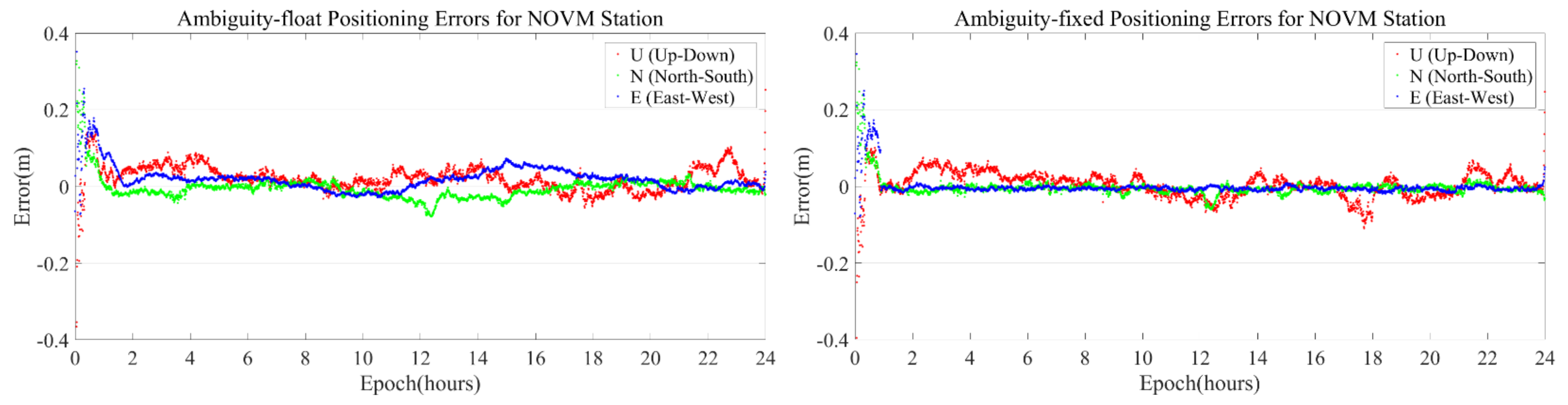
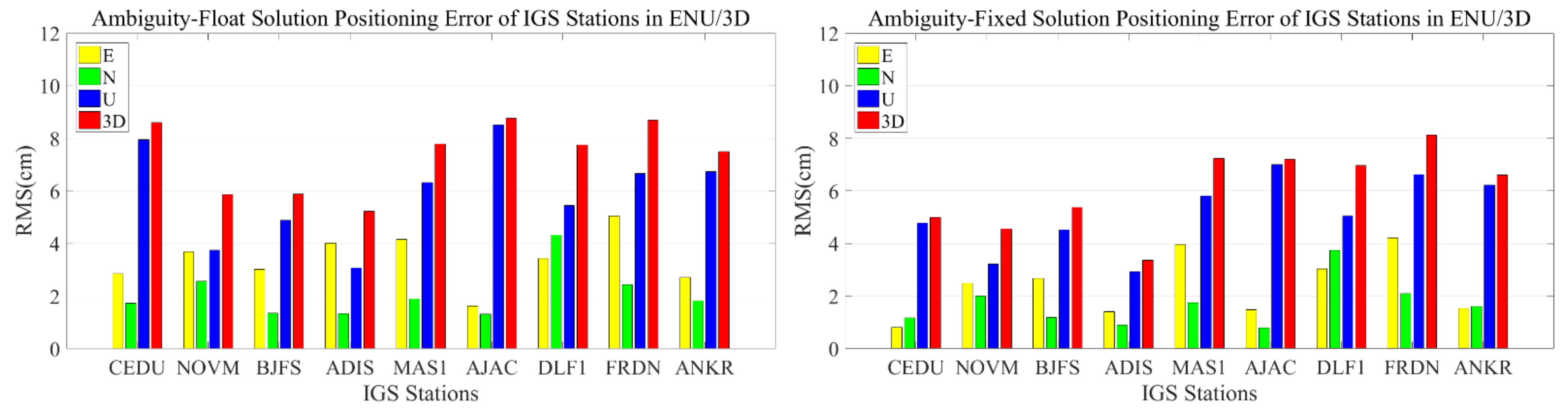
4.1. Validation Results of Real-Time Ambiguity Resolution for PPP

In this section, the real-time ambiguity-resolution algorithm for kinematic PPP is validated with nine randomly selected IGS stations and 10 days of data from 15 to 24 January 2017. Taking two IGS stations, CEDU and NOVM, on 15 January 2017 as examples, the time series of position errors between the ambiguity-float or ambiguity-fixed solutions and IGS-released data are shown in Figure 2 and Figure 3, respectively. It should be noted that the ambiguity-float and the ambiguity-fixed solution, respectively, indicate whether the ambiguity parameter is calculated in the form of a decimal-point number or an integer. The time series of position errors in E (east-west), N (north-south), and U (up-down) directions are denoted by blue, green, and red lines. It can be found from Figure 2 and Figure 3 that the positioning accuracy of real-time PPP ambiguity resolution is better than that of traditional float PPP, not only in the E direction but also in the N and U directions.

Table 2. The ambiguity-fixed ratio and RMS of real-time PPP in E (east-west), N (north-south), and U (up-down) directions and 3D-RMS (total position error) with different solution types.

IGS Station	Solution Type	RMS (cm)				Fixed Ratio	Precision Improvement of 3D-RMS
		E	N	U	3D-RMS
CEDU	Float	2.85	1.73	7.94	8.61	96.3%	↑ 42%
	Fix	0.80	1.17	4.78	4.99
NOVM	Float	3.69	2.57	3.75	5.86	96.2%	↑ 22%
	Fix	2.50	2.01	3.22	4.55
BJFS	Float	3.01	1.35	4.88	5.89	94.3%	↑ 9%
	Fix	2.67	1.18	4.52	5.38
ADIS	Float	4.02	1.34	3.07	5.23	97.1%	↑ 36%
	Fix	1.41	0.90	2.93	3.37
MAS1	Float	4.16	1.89	6.31	7.79	94.8%	↑ 7%
	Fix	3.96	1.75	5.81	7.25
AJAC	Float	1.63	1.32	8.51	8.76	95.7%	↑ 18%
	Fix	1.48	0.79	7.00	7.20
DLF1	Float	3.43	4.32	5.45	7.75	94.4%	↑ 10%
	Fix	3.04	3.74	5.04	6.97
FRDN	Float	5.04	2.43	6.66	8.70	89.3%	↑ 7%
	Fix	4.22	2.10	6.62	8.13
ANKR	Float	2.71	1.82	6.74	7.49	98.0%	↑ 12%
	Fix	1.53	1.61	6.23	6.61
Average	Float	3.39	2.09	5.92	7.14	95.1%	↑ 17%
	Fix	2.40	1.69	5.13	5.91

illustrates the ambiguity-fixed ratio and the accuracy of real-time PPP with ambiguity-float and ambiguity-fixed solutions. It should be pointed out that the ambiguity-fixed ratio represents the rate of the number of epochs for which the ambiguity parameters are successfully fixed as integers to the total number of epochs. It can be found in Table 2 that the total position error (3D-RMS) of both PPP ambiguity resolution and float PPP can achieve a positioning error within 10 cm. The most obvious improvement of the average accuracy is in the E direction, from 3.39 cm to 2.40 cm, with an enhancement of around 29%. The respective improvement of the N and U directions is about 19% and 13%. Besides, compared with real-time float PPP, the average accuracy of PPP ambiguity-resolution positioning error is enhanced by approximately 17%, and the average ambiguity-fixed ratio is about 95.1%. It should be pointed out that the average improvement of IGS stations in the vertical direction (the U direction) is about 13%, which is markedly worse than that of the horizontal directions (the improvement of E and N directions is around 29% and 19%, respectively). The reason could be that the vertical component has a strong correlation with the receiver-clock and the zenith wet-delay parameter during parameter estimation and absorbs the errors belonging to the receiver clock and the zenith wet delay [52]. In addition, the phase biases have been demonstrated to be more correlated with the horizontal direction than with the vertical direction [40,42]. In the two horizontal directions, because of the north-south ground tracks of GPS satellites at the equator in the Earth-fixed reference frame, the phase biases are more correlated with the east-west component than with the north-south [40]. Thus, after the ambiguity parameter is successfully recovered to an integer, the improvement of accuracy in the E direction is most significant, while the accuracy in the U direction is improved least. Meanwhile, the average accuracy of IGS station positioning error with real-time PPP ambiguity resolution and float PPP is given in Figure 4, where the RMS of E, N, U, and 3D are represented by the yellow, green, blue, and red bars, respectively.

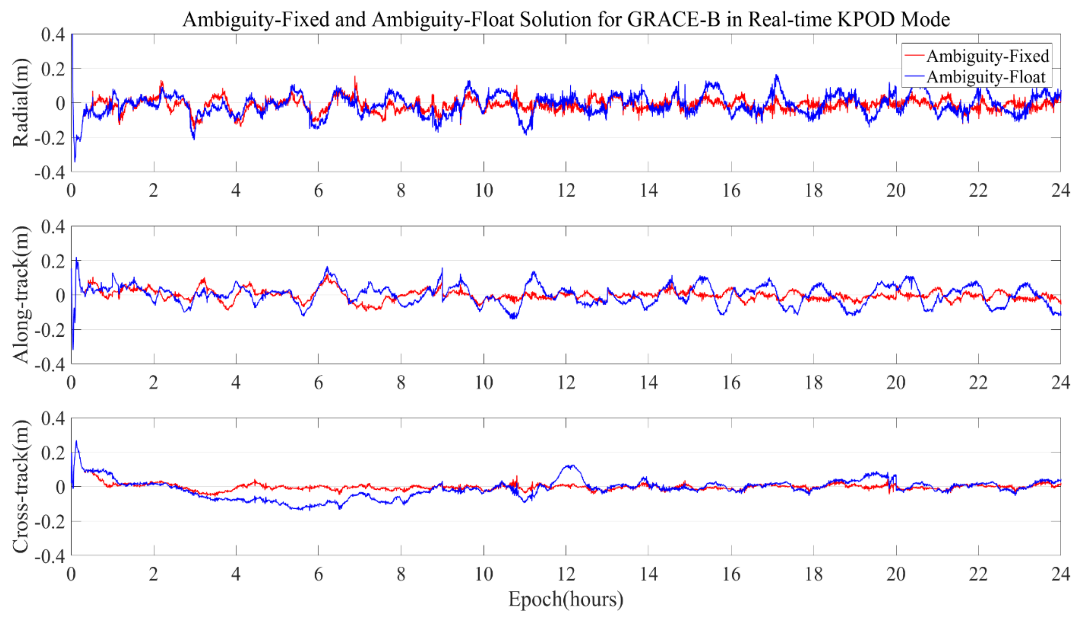
4.2. Validation Results of Real-Time Ambiguity Resolution for LEO KPOD

In this section, the spaceborne data of GRACE series satellites are used to verify the performance of real-time LEO KPOD with ambiguity resolution and compare with float KPOD for GRACE satellites. Ten days of onboard observations from 15 January 2017 to 24 January 2017 were used in this experiment. Figure 5 displays the time series of orbit differences between the real-time KPOD for GRACE-B and reference orbits on 15 January 2017, where the differences are shown in radial (R), along-track (A), and cross-track (C) directions, respectively. Reference orbits as real values are calculated by post-processed RPOD from the JPL (Jet Propulsion Laboratory), which can be obtained from the Information System and Data Centre (ISDC). Additionally, the orbital time series of differences with ambiguity-fixed and ambiguity-float solutions are denoted by red lines and blue lines, respectively. It can be found in Figure 5 that orbital differences of real-time KPOD with ambiguity resolution are better than those of the float KPOD mode in R, A, and C directions after ambiguities are recovered as integers. Meanwhile, compared with the real-time KOPD with ambiguity-float solutions, the differences of orbit in ambiguity-fixed solutions perform smaller fluctuations.

We further conducted statistics on the real-time KPOD accuracies of all participating experiments, which are shown in Figure 6. The upper sub-figure and bottom sub-figure exhibited in Figure 6 represent the result of the real-time KPOD with ambiguity-float and ambiguity-fixed solutions, respectively. The real-time KPOD accuracies and the date of experiments are depicted by the ordinate axis and the abscissa axis, respectively. The accuracies of different directions, i.e., the R, A, and C directions and 3D, of real-time KPOD are displayed with different colors denoted by yellow, green, blue, and red, respectively.

More details about the ambiguity-float and ambiguity-fixed solution of GRACE-B with real-time KPOD mode are shown in

Table 3. The GRACE-B ambiguity-fixed ratio and RMS of real-time KPOD in R (radial), A (along-track), and C (cross-track) directions and 3D-RMS (total position error) with different solution types.

GRACE-B.
Time	Method	Solution Type	RMS (cm)				Fixed Ratio	Precision Improvement of 3D-RMS
			R	A	C	3D-RMS
20170115	KPOD	Float	7.06	4.77	4.45	9.61	94.1%	↑ 21%
		Fix	6.32	3.39	2.56	7.61
20170116	KPOD	Float	6.31	4.02	3.21	8.14	90.4%	↑ 17%
		Fix	4.87	3.62	2.98	6.76
20170117	KPOD	Float	6.91	4.96	3.89	9.35	92.7%	↑ 15%
		Fix	6.37	3.52	3.14	7.93
20170118	KPOD	Float	7.03	3.88	2.54	8.42	94.8%	↑ 22%
		Fix	4.72	3.61	2.83	6.58
20170119	KPOD	Float	7.81	6.04	3.32	10.42	89.8%	↑ 11%
		Fix	6.82	5.52	3.15	9.32
20170120	KPOD	Float	4.94	4.31	3.92	7.64	91.9%	↑ 16%
		Fix	3.88	3.67	3.57	6.42
20170121	KPOD	Float	5.42	4.04	3.96	7.83	90.8%	↑ 15%
		Fix	4.61	3.14	3.61	6.64
20170122	KPOD	Float	5.44	3.65	3.47	7.41	91.5%	↑ 15%
		Fix	4.57	3.32	2.79	6.30
20170123	KPOD	Float	5.78	4.39	3.84	8.21	89.1%	↑ 17%
		Fix	4.61	3.74	3.31	6.80
20170124	KPOD	Float	4.83	3.95	4.66	7.79	93.4%	↑ 18%
		Fix	3.88	3.35	3.76	6.36
Average	KPOP	Float	6.05	4.40	3.73	8.36	91.9%	↑ 16%
		Fix	5.07	3.69	3.17	7.02

. Both accuracies of KPOD with the ambiguity-fixed and ambiguity-float solutions were able to reach the sub-decimeter level (around 6–10 cm) during the test period. However, the average accuracy of ambiguity resolution is better than that of the float solutions. The orbital 3D-RMS of GRACE-B reduced from 8.36 cm to 7.02 cm, compared with the ambiguity-float solution. Regarding the ambiguity-fixed ratio in the test period, the fixed ratio varies from 89.1% to 94.8%, and the average ambiguity-fixed ratio is 91.9%. Moreover, the 3D-RMS average orbital accuracy improvement is around 16%.

The accuracy of real-time KPOD for GRACE-A by applying the ambiguity-float and ambiguity-fixed solutions are illustrated in Figure 7, and it can be found that the 3D-RMS of real-time KPOD, both with ambiguity-float solutions and ambiguity-fixed solutions, is better than 10 cm. The orbital accuracy of the ambiguity-fixed solution for GRACE-A in each direction is better than that of the ambiguity-float solution during the processing period.

Table 4. The GRACE-A ambiguity-fixed ratio and RMS of real-time KPOD in R (radial), A (along-track), an C (cross-track) directions and 3D-RMS (total position error) with different solution types.

GRACE-A
Time	Method	Solution Type	RMS (cm)				Fixed Ratio	Precision Improvement of 3D-RMS
			R	A	C	3D-RMS
20170115	KPOD	Float	5.98	4.21	3.12	7.95	92.1%	↑ 14%
		Fix	4.81	3.88	2.94	6.84
20170116	KPOD	Float	7.31	4.53	3.66	9.35	93.6%	↑ 16%
		Fix	6.33	3.4	3.14	7.84
20170117	KPOD	Float	6.41	3.89	3.32	8.20	92.4%	↑ 17%
		Fix	4.52	3.92	3.21	6.79
20170118	KPOD	Float	4.88	4.36	3.62	7.48	94.2%	↑ 18%
		Fix	3.74	3.71	3.15	6.14
20170119	KPOD	Float	5.01	3.94	4.02	7.54	91.8%	↑ 15%
		Fix	4.08	3.56	3.44	6.42
20170120	KPOD	Float	5.64	3.88	3.67	7.77	94.6%	↑ 18%
		Fix	4.41	2.99	3.5	6.37
20170121	KPOD	Float	5.79	3.86	3.62	7.84	95.3%	↑ 20%
		Fix	4.36	3.48	2.84	6.26
20170122	KPOD	Float	5.22	4.54	3.81	7.90	93.3%	↑ 16%
		Fix	4.44	3.73	3.19	6.62
20170123	KPOD	Float	5.53	4.9	4.33	8.56	90.5%	↑ 14%
		Fix	4.31	4.4	4.03	7.36
20170124	KPOD	Float	7.24	5.88	3.41	9.93	90.7%	↑ 10%
		Fix	6.44	5.41	3.02	8.94
Average	KPOD	Float	5.90	4.40	3.66	8.22	92.9%	↑ 16%
		Fix	4.74	3.85	3.25	6.92

gives more comprehensive statistical information, including the accuracy of the real-time KPOD involved in the experiment, the fixed ratio of ambiguity, and the improvement of accuracy. The average RMS improvement of the ambiguity-fixed solution for GRACE-A in the radial, along-track, and cross-track directions relative to that of traditional-float KPOD is around 20%, 13%, and 11%, respectively. In addition, the average daily ambiguity-fixed ratio and 3D-RMS improvement compared with the float solution are 92.9% and 16%, respectively. Therefore, it has been demonstrated that the ambiguity resolution applied in the real-time KPOD for LEO can be considered an effective method to strengthen the observation model and improve the accuracy of POD.

4.3. Validation Results of Real-Time Ambiguity Resolution for LEO RPOD

In this section, the real-time RPOD is computed for GRACE satellites by employing the ambiguity-fixed and ambiguity-float solution to verify the performance of LEO POD. The orbital differences time series between the result of real-time RPOD and reference orbit in radial, along-track, and cross-track directions for GRACE-B on 15.01.2017 are depicted in Figure 8, where the abscissa axis and the ordinate axis are observation time and the orbital difference between RPOD and reference orbits, respectively. A phenomenon similar to real-time KPOD can be drawn from Figure 8 that the performance of ambiguity-fixed is better than that of ambiguity-float in the RPOD mode. Figure 9 gives the result of RPOD for GRACE-B with ambiguity-float (upper sub-figure) and ambiguity-fixed (bottom sub-figure) solutions. It can be seen that the 3D accuracy of fixed-ambiguity and float ambiguity-solutions are better than 9 cm and 8 cm, respectively, in real-time RPOD mode for the data used in our experiment.

Table 5. The GRACE-B ambiguity-fixed ratio and RMS of real-time RPOD in R (radial), A (along-track), and C(cross-track) directions and 3D-RMS (total position error) with different solution types.

GRACE-B
Time	Method	Solution Type	RMS (cm)				Fixed Ratio	Precision Improvement of 3D-RMS
			R	A	C	3D-RMS
20170115	RPOD	Float	6.31	4.27	2.61	8.05	95.4%	↑ 13%
		Fix	6.05	3.23	1.58	7.04
20170116	RPOD	Float	5.21	3.76	2.96	7.07	91.1%	↑ 9%
		Fix	4.65	3.51	2.79	6.46
20170117	RPOD	Float	6.63	4.13	3.54	8.58	93.6%	↑ 12%
		Fix	6.18	3.31	2.89	7.58
20170118	RPOD	Float	6.27	3.61	2.32	7.60	96.1%	↑ 16%
		Fix	4.57	3.52	2.71	6.37
20170119	RPOD	Float	7.01	4.59	3.03	8.91	90.4%	↑ 9%
		Fix	6.23	4.22	2.98	8.09
20170120	RPOD	Float	4.43	3.62	3.82	6.88	92.4%	↑ 12%
		Fix	3.79	3.51	3.19	6.07
20170121	RPOD	Float	4.61	3.24	3.41	6.59	90.7%	↑ 7%
		Fix	4.21	2.99	3.32	6.14
20170122	RPOD	Float	4.73	3.35	3.05	6.55	93.1%	↑ 11%
		Fix	4.16	3.10	2.65	5.83
20170123	RPOD	Float	4.71	3.94	3.13	6.89	89.7%	↑ 9%
		Fix	4.25	3.54	3.02	6.30
20170124	RPOD	Float	4.05	3.17	4.15	6.61	93.8%	↑ 13%
		Fix	3.43	2.95	3.56	5.76
Average	RPOD	Float	5.40	3.77	3.20	7.32	92.6%	↑ 11%
		Fix	4.75	3.39	2.87	6.50

lists the real-time RPOD solution type, RMS in radial, along-track, and cross-track directions, ambiguity-fixed ratio, and precision improvement. The average 3D-RMS of ambiguity-float and ambiguity-fixed solutions is 7.32 cm and 6.50 cm, respectively. In the real-time RPOD mode, the average accuracy of fixed ambiguity for GRACE-B is improved by 11% relative to that of ambiguity-float solutions. The respective improvement in the radial, along-track, and cross-track directions are 12%, 10%, and 10%. Nevertheless, the accuracy improvement of RPOD with ambiguity resolution is not as much as that of real-time KPOD mode. One of the primary reasons is that the accuracy of real-time RPOD with the constraints of the dynamic model is higher than that of KPOD without the constraints of the dynamic model. Thus, the accuracy after the ambiguity is fixed in the RKOD mode is not as obviously improved as that of the KPOD mode.

The statistical results of the real-time RPOD with ambiguity-float and ambiguity-fixed solutions for GRACE-A are exhibited in Figure 10 and

Table 6. The GRACE-A ambiguity-fixed ratio and RMS of real-time RPOD in R (radial), A (along-track), and C (cross-track) directions and 3D-RMS (total position error) with different solution types.

GRACE-A
Time	Method	Solution Type	RMS (cm)				Fixed Ratio	Precision Improvement of 3D-RMS
			R	A	C	3D-RMS
20170115	RPOD	Float	5.31	3.81	2.99	7.19	93.0%	↑ 9%
		Fix	4.67	3.61	2.85	6.55
20170116	RPOD	Float	6.93	4.32	3.41	8.85	94.3%	↑ 13%
		Fix	6.24	3.31	3.06	7.70
20170117	RPOD	Float	6.11	3.58	2.28	7.44	93.9%	↑ 12%
		Fix	4.32	3.84	3.11	6.56
20170118	RPOD	Float	4.17	4.01	3.18	6.60	91.6%	↑ 11%
		Fix	3.61	3.55	3.02	5.90
20170119	RPOD	Float	4.31	3.57	3.75	6.74	92.0%	↑ 9%
		Fix	3.88	3.48	3.21	6.12
20170120	RPOD	Float	4.79	3.35	3.41	6.77	95.1%	↑ 8%
		Fix	4.32	2.94	3.43	6.25
20170121	RPOD	Float	4.83	3.46	2.96	6.64	96.8%	↑ 9%
		Fix	4.25	3.32	2.79	6.07
20170122	RPOD	Float	4.71	3.94	3.13	6.89	94.5%	↑ 7%
		Fix	4.3	3.62	3.05	6.40
20170123	RPOD	Float	6.01	4.81	3.02	8.27	92.2%	↑ 12%
		Fix	5.23	4.12	2.89	7.26
20170124	RPOD	Float	4.32	4.21	3.26	6.86	94.9%	↑ 13%
		Fix	3.61	3.64	3.03	5.96
Average	RPOD	Float	5.15	3.91	3.14	7.18	93.8%	↑ 10%
		Fix	4.44	3.54	3.04	6.45

. The real-time results of RPOD for GRACE-A by employing ambiguity-fixed and ambiguity-float solutions are better than 10 cm in Figure 10. It can be found in Table 6 that the ambiguity-fixed ratio can reach more than 90% during the processing period, and regarding the accuracy improvement, after the ambiguities are successfully fixed as integers, the improvement varies from 7% to 13%. Thus, the ambiguity resolution, by applying IPC and WSB products, improves the accuracy of both real-time KPOD and RPOD mode for GRACE series satellites.

5. Conclusions

The real-time onboard POD for LEO with ambiguity resolution is an effective method to strengthen the observation model and improve the performance of orbit determination. To verify the effectiveness of single-receiver carrier-phase integer-ambiguity resolution on real-time PPP, KPOD, and RPOD, a methodology of ambiguity resolution based on IPC and wide-lane satellite-bias products from CNES has been briefly introduced in this work. Furthermore, the ambiguity resolution of real-time PPP, LEO KPOD, and RPOD are validated by applying the data from IGS stations and multiple GRACE satellites, respectively. The conclusions are shown below:

• The average accuracy of positioning error (3D-RMS) for the real-time PPP, both with ambiguity-fixed and ambiguity-float solutions, can achieve centimeter-level accuracy. Compared with the float PPP solutions, the average positioning errors of ambiguity-fixed solutions in the horizontal and vertical directions are improved by 26% and 13%, respectively, the accuracy improvement in the east-west direction is the most significant, at about 29%.
• After applying the integer-ambiguity resolution to the real-time KPOD mode for GRACE series satellites, the average accuracies (3D-RMS) of GRACE-A and GRACE-B in the abovementioned mode are about 6.92 cm and 7.02 cm, respectively. In comparison with real-time KPOD with ambiguity-float solutions, the average improvement in position for these two satellites, GRACE-A and GRACE-B, is approximately 16%.
• In the real-time RPOD mode, a comparison of orbital accuracy between ambiguity-float and ambiguity-fixed solutions for GRACE satellites shows that the average real-time RPOD accuracy (3D-RMS) with ambiguity-fixed solutions is better (about 10%) than that with float solutions. Regardless of fixed- or float-ambiguity solutions, the performance of real-time RPOD is better than that of the corresponding KPOD. However, when the constraints of the dynamic model are applied in real-time RPOD mode, the increase in the accuracy under the real-time RPOD mode is not as obvious as under the real-time KPOD mode without the constraints of the dynamic model. Moreover, the average ambiguity-fixing ratio in the real-time PPP, KPOD, and RPOD was above 90% during the test period.

References

1. Chen, C.-R.; Hwang, F.-T.; Hsueh, C.-W. Mission Studies on Constellation of Leo Satellites with Remote-Sensing and Communication Payloads. In Earth Observing Systems XXII; International Society for Optics and Photonics: San Diego, CA, USA, 2017; p. 1040207. [Google Scholar]
2. Ravanbakhsh, A.; Franchini, S. System engineering approach to initial design of leo remote sensing missions. In Proceedings of the 2013 6th International Conference on Recent Advances in Space Technologies (RAST), Istanbul, Turkey, 12–14 June 2013; pp. 659–664. [Google Scholar]
3. Gagliardi, F.; Vaccaro, A.; Villacci, D. Performance analysis of leo satellites based communication systems for remote monitoring and protection of power components. In Proceedings of the 2003 IEEE Bologna Power Tech Conference Proceedings, Bologna, Italy, 23–26 June 2003; Volume 2, p. 6. [Google Scholar]
4. Pelton, J.N.; Madry, S.; Camacho-Lara, S. Satellite applications handbook: The complete guide to satellite communications, remote sensing, navigation, and meteorology. In Handbook of Satellite Application; Springer: New York, NY, USA, 2013; pp. 3–19. [Google Scholar]
5. König, R.; Zhu, S.; Reigber, C.; Neumayer, K.-H.; Meixner, H.; Galas, R.; Baustert, G.; Schwintzer, P. Champ rapid orbit determination for gps atmospheric limb sounding. Adv. Space Res. 2002, 30, 289–293. [Google Scholar] [CrossRef]
6. Wickert, J.; Beyerle, G.; König, R.; Heise, S.; Grunwaldt, L.; Michalak, G.; Reigber, C.; Schmidt, T. Gps radio occultation with champ and grace: A first look at a new and promising satellite configuration for global atmospheric sounding. In Annales Geophysicae; Copernicus GmbH: Göttingen, Germany, 2005; pp. 653–658. [Google Scholar]
7. Kursinski, E.; Hajj, G.; Schofield, J.; Linfield, R.; Hardy, K.R. Observing earth’s atmosphere with radio occultation measurements using the global positioning system. J. Geophys. Res. Atmos. 1997, 102, 23429–23465. [Google Scholar] [CrossRef]
8. Wickert, J.; Reigber, C.; Beyerle, G.; König, R.; Marquardt, C.; Schmidt, T.; Grunwaldt, L.; Galas, R.; Meehan, T.K.; Melbourne, W.G. Atmosphere sounding by gps radio occultation: First results from champ. Geophys. Res. Lett. 2001, 28, 3263–3266. [Google Scholar] [CrossRef] [Green Version]
9. Cerri, L.; Berthias, J.; Bertiger, W.; Haines, B.; Lemoine, F.; Mercier, F.; Ries, J.; Willis, P.; Zelensky, N.; Ziebart, M. Precision orbit determination standards for the jason series of altimeter missions. Mar. Geod. 2010, 33, 379–418. [Google Scholar] [CrossRef]
10. Martín-Neira, M.; D’Addio, S.; Buck, C.; Floury, N.; Prieto-Cerdeira, R. The paris ocean altimeter in-orbit demonstrator. IEEE Trans. Geosci. Remote Sens. 2011, 49, 2209–2237. [Google Scholar] [CrossRef]
11. Li, B.; Ge, H.; Ge, M.; Nie, L.; Shen, Y.; Schuh, H. Leo enhanced global navigation satellite system (legnss) for real-time precise positioning services. Adv. Space Res. 2019, 63, 73–93. [Google Scholar] [CrossRef]
12. Li, X.; Dick, G.; Lu, C.; Ge, M.; Nilsson, T.; Ning, T.; Wickert, J.; Schuh, H. Multi-gnss meteorology: Real-time retrieving of atmospheric water vapor from beidou, galileo, glonass, and gps observations. IEEE Trans. Geosci. Remote Sens. 2015, 53, 6385–6393. [Google Scholar] [CrossRef] [Green Version]
13. Hadas, T.; Bosy, J. Igs rts precise orbits and clocks verification and quality degradation over time. GPS Solut. 2015, 19, 93–105. [Google Scholar] [CrossRef] [Green Version]
14. Wang, Z.; Li, Z.; Wang, L.; Wang, N.; Yang, Y.; Li, R.; Zhang, Y.; Liu, A.; Yuan, H.; Hoque, M. Comparison of the real-time precise orbit determination for leo between kinematic and reduced-dynamic modes. Measurement 2021, 187, 110224. [Google Scholar] [CrossRef]
15. Hauschild, A.; Tegedor, J.; Montenbruck, O.; Visser, H.; Markgraf, M. Precise onboard orbit determination for leo satellites with real-time orbit and clock corrections. In Proceedings of the 29th International Technical Meeting of the Satellite Division of the Institute of Navigation (ION GNSS+ 2016), Portland, OR, USA, 12–16 September 2016; pp. 3715–3723. [Google Scholar]
16. Liu, C.; Gao, W.; Liu, T.; Wang, D.; Yao, Z.; Gao, Y.; Nie, X.; Wang, W.; Li, D.; Zhang, W. Design and implementation of a bds precise point positioning service. Navig. J. Inst. Navig. 2020, 67, 875–891. [Google Scholar] [CrossRef]
17. Yang, Y.; Mao, Y.; Sun, B. Basic performance and future developments of beidou global navigation satellite system. Satell. Navig. 2020, 1, 1. [Google Scholar] [CrossRef] [Green Version]
18. Allahvirdi-Zadeh, A.; Wang, K.; El-Mowafy, A. Pod of small leo satellites based on precise real-time madoca and sbas-aided ppp corrections. GPS Solut. 2021, 25, 31. [Google Scholar] [CrossRef]
19. Miya, M.; Fujita, S.; Sato, Y.; Kaneko, K.; Shima, Y.; Hirokawa, R.; Sone, H.; Takiguchi, J.-I. Centimeter level augmentation service (clas) in japanese quasi-zenith satellite system, design for satellite based rtk-ppp services. In Proceedings of the 28th International Technical Meeting of the Satellite Division of the Institute of Navigation (ION GNSS+ 2015), Tampa, FL, USA, 14–18 September 2015; pp. 1958–1962. [Google Scholar]
20. Chatre, E.; Benedicto, J. 2019–galileo programme update. In Proceedings of the 32nd International Technical Meeting of the Satellite Division of The Institute of Navigation (ION GNSS+ 2019), Miami, FL, USA, 16–20 September 2019; pp. 650–698. [Google Scholar]
21. Wu, S.-C.; Yunck, T.P.; Thornton, C.L. Reduced-dynamic technique for precise orbit determination of low earth satellites. J. Guid. Control Dyn. 1991, 14, 24–30. [Google Scholar] [CrossRef]
22. Švehla, D.; Rothacher, M. Kinematic and reduced-dynamic precise orbit determination of low earth orbiters. Adv. Geosci. 2003, 1, 47–56. [Google Scholar] [CrossRef] [Green Version]
23. Li, X.; Wu, J.; Zhang, K.; Li, X.; Xiong, Y.; Zhang, Q. Real-time kinematic precise orbit determination for leo satellites using zero-differenced ambiguity resolution. Remote Sens. 2019, 11, 2815. [Google Scholar] [CrossRef] [Green Version]
24. Geng, J.; Teferle, F.N.; Shi, C.; Meng, X.; Dodson, A.; Liu, J. Ambiguity resolution in precise point positioning with hourly data. GPS Solut. 2009, 13, 263–270. [Google Scholar] [CrossRef] [Green Version]
25. Jäggi, A.; Hugentobler, U.; Bock, H.; Beutler, G. Precise orbit determination for grace using undifferenced or doubly differenced gps data. Adv. Space Res. 2007, 39, 1612–1619. [Google Scholar] [CrossRef]
26. Ge, M.; Gendt, G.; Rothacher, M.a.; Shi, C.; Liu, J. Resolution of gps carrier-phase ambiguities in precise point positioning (ppp) with daily observations. J. Geod. 2008, 82, 389–399. [Google Scholar] [CrossRef]
27. Laurichesse, D.; Mercier, F.; Berthias, J.P.; Broca, P.; Cerri, L. Integer ambiguity resolution on undifferenced gps phase measurements and its application to ppp and satellite precise orbit determination. Navigation 2009, 56, 135–149. [Google Scholar] [CrossRef]
28. Chen, X. An alternative integer recovery clock method for precise point positioning with ambiguity resolution. Satell. Navig. 2020, 1, 28. [Google Scholar] [CrossRef]
29. Loyer, S.; Perosanz, F.; Mercier, F.; Capdeville, H.; Marty, J.-C. Zero-difference gps ambiguity resolution at cnes–cls igs analysis center. J. Geod. 2012, 86, 991–1003. [Google Scholar] [CrossRef]
30. Katsigianni, G.; Loyer, S.; Perosanz, F.; Mercier, F.; Zajdel, R.; Sośnica, K. Improving galileo orbit determination using zero-difference ambiguity fixing in a multi-gnss processing. Adv. Space Res. 2019, 63, 2952–2963. [Google Scholar] [CrossRef]
31. Montenbruck, O.; Hackel, S.; van den Ijssel, J.; Arnold, D. Reduced dynamic and kinematic precise orbit determination for the swarm mission from 4 years of gps tracking. GPS Solut. 2018, 22, 79. [Google Scholar] [CrossRef]
32. Hofmann-Wellenhof, B.; Lichtenegger, H.; Wasle, E. Gnss–Global Navigation Satellite Systems: Gps, Glonass, Galileo, and More; Springer Science & Business Media: Berlin/Heidelberg, Germany, 2007. [Google Scholar]
33. Teunissen, P.; Montenbruck, O. Springer Handbook of Global Navigation Satellite Systems; Springer: Berlin/Heidelberg, Germany, 2017. [Google Scholar]
34. Wang, Z.; Li, Z.; Wang, L.; Wang, X.; Yuan, H. Assessment of multiple gnss real-time ssr products from different analysis centers. ISPRS Int. J. Geo-Inf. 2018, 7, 85. [Google Scholar] [CrossRef] [Green Version]
35. Zhan, Y. Comparison between uofc model and ionosphere-free combination model in ppp. In Journal of Physics: Conference Series; IOP Publishing: Bristol, UK, 2019; p. 022060. [Google Scholar]
36. An, X.; Meng, X.; Jiang, W. Multi-constellation gnss precise point positioning with multi-frequency raw observations and dual-frequency observations of ionospheric-free linear combination. Satell. Navig. 2020, 1, 7. [Google Scholar] [CrossRef]
37. Li, R.; Li, Z.; Wang, N.; Tang, C.; Ma, H.; Zhang, Y.; Wang, Z.; Wu, J. Considering inter-receiver pseudorange biases for bds-2 precise orbit determination. Measurement 2021, 177, 109251. [Google Scholar] [CrossRef]
38. Yang, Y.; Yue, X.; Yuan, J. Gps based reduced-dynamic orbit determination for low earth orbiters with ambiguity fixing. Int. J. Aerosp. Eng. 2015, 2015, 723414. [Google Scholar] [CrossRef] [Green Version]
39. Li, R.; Wang, N.; Li, Z.; Zhang, Y.; Wang, Z.; Ma, H. Precise orbit determination of bds-3 satellites using b1c and b2a dual-frequency measurements. GPS Solut. 2021, 25, 95. [Google Scholar] [CrossRef]
40. Melbourne, W.G. The case for ranging in gps-based geodetic systems. In Proceedings of the First International Symposium on Precise Positioning with the Global Positioning System, US Department of Commerce, Rockville, MD, USA, 15–19 April 1985; pp. 373–386. [Google Scholar]
41. Wübbena, G. Software developments for geodetic positioning with gps using ti4100 code and carrier measurements. In Proceedings of the 1st International Symposium on Precise Positioning with the Global Positioning System, Rockville, MD, USA, 15–19 April 1985; pp. 403–412. [Google Scholar]
42. Blewitt, G. Carrier phase ambiguity resolution for the global positioning system applied to geodetic baselines up to 2000 km. J. Geophys. Res. Solid Earth 1989, 94, 10187–10203. [Google Scholar] [CrossRef] [Green Version]
43. Dong, D.N.; Bock, Y. Global positioning system network analysis with phase ambiguity resolution applied to crustal deformation studies in california. J. Geophys. Res. Solid Earth 1989, 94, 3949–3966. [Google Scholar] [CrossRef]
44. Katsigianni, G.; Loyer, S.; Perosanz, F. Ppp and ppp-ar kinematic post-processed performance of gps-only, galileo-only and multi-gnss. Remote Sens. 2019, 11, 2477. [Google Scholar] [CrossRef] [Green Version]
45. MarFn, A.; Hadas, T.; Dimas, A.; Anquela, A.; Berne, J. Influence of real-time products latency on kinematic ppp results. In Proceedings of the ESA 5th International Colloquium on Scientific and Fundamental Aspects of the Galileo Program, Braunschweig, Germany, 27–29 October 2015. [Google Scholar]
46. Montenbruck, O.; Gill, E.; Lutze, F. Satellite orbits: Models, methods, and applications. Appl. Mech. Rev. 2002, 55, B27–B28. [Google Scholar] [CrossRef]
47. Svehla, D. Integer ambiguity algebra. In Geometrical Theory of Satellite Orbits and Gravity Field; Springer: Berlin/Heidelberg, Germany, 2018; pp. 319–354. [Google Scholar]
48. Wu, J.-T.; Wu, S.C.; Hajj, G.A.; Bertiger, W.I.; Lichten, S.M. Effects of antenna orientation on gps carrier phase. Manuscripta Geodaetica 1993, 18, 91–98. [Google Scholar]
49. Kouba, J. A Guide to Using International Gnss Service (IGS) Products; IGS Central Bureau: Pasadena, CA, USA, 2009. Available online: http://igscb.jpl.nasa.gov/igscb/resource/pubs/GuidetoUsingIGSProducts.pdf (accessed on 6 December 2020).
50. Ries, J.; Bettadpur, S.; Eanes, R.; Kang, Z.; Ko, U.-d.; McCullough, C.; Nagel, P.; Pie, N.; Poole, S.; Richter, T. The Development and Evaluation of the Global Gravity Model ggm05; Center for Space Research, The University of Texas: Austin, TX, USA, 2016. [Google Scholar] [CrossRef]
51. Bizouard, C.; Lambert, S.; Gattano, C.; Becker, O.; Richard, J.-Y. The iers eop 14c04 solution for earth orientation parameters consistent with itrf 2014. J. Geod. 2019, 93, 621–633. [Google Scholar] [CrossRef]
52. Xiao, G. Multi-Frequency and Multi-Gnss ppp Phase Bias Estimation and Ambiguity Resolution; Karlsruher Institut für Technologie (KIT): Karlsruhe, Germany, 2019. [Google Scholar]
Figure 1. Flow chart of ambiguity resolution for real-time PPP/LEO POD.
Aerospace 09 00025 g001
Figure 2. The time series of CEDU station position errors between the ambiguity-float (left subgraph) or ambiguity-fixed (right subgraph) solution and IGS-released data.
Aerospace 09 00025 g002
Figure 3. The time series of NOVM station position errors between the ambiguity-float (left subgraph) or ambiguity-fixed (right subgraph) solution and IGS-released data.
Aerospace 09 00025 g003
Figure 4. IGS station average positioning error of ambiguity-float (left) and ambiguity-fixed (right) solutions in E, N, and U directions and 3D-RMS.
Aerospace 09 00025 g004
Figure 5. Orbital differences of GRACE-B ambiguity-fixed and ambiguity-float KPOD based on comparison with reference orbits.
Aerospace 09 00025 g005
Figure 6. The accuracy (RMS) of real-time KPOD ambiguity-float (upper) and ambiguity-fixed (bottom) solution for GRACE-B.
Aerospace 09 00025 g006
Figure 7. The accuracy (RMS) of real-time KPOD ambiguity-float (upper) and ambiguity-fixed (bottom) solution for GRACE-A.
Aerospace 09 00025 g007
Figure 8. Orbital differences of GRACE-B ambiguity-fixed and ambiguity-float RPOD based on comparison with reference orbits.
Aerospace 09 00025 g008
Figure 9. The accuracy (RMS) of real-time RPOD ambiguity-float (upper) and ambiguity-fixed (bottom) solution for GRACE-B.
Aerospace 09 00025 g009
Figure 10. The accuracy (RMS) of real-time RPOD ambiguity-float (upper) and ambiguity-fixed (bottom) solution for GRACE-A.
Aerospace 09 00025 g010