
Quaternion versus Rotation Matrix Feedback for Spacecraft Attitude Stabilization Using Magnetorquers †


School of Aerospace Engineering, Sapienza University of Rome, via Salaria 851, 00138 Roma, Italy
†
This paper is an extended version of my paper published in Fifth IAA Conference on University Satellite Missions and Cubesat Workshop 2020, Rome, Italy, 28–31 January 2020.
Aerospace 2022, 9(1), 24; https://doi.org/10.3390/aerospace9010024
Submission received: 8 December 2021
/
Revised: 27 December 2021
/
Accepted: 29 December 2021
/
Published: 4 January 2022
(This article belongs to the Special Issue Spacecraft Attitude Control Using Magnetic Actuators)
Abstract
:The purpose of this paper is to compare performances between stabilization algorithms of quaternion plus attitude rate feedback and rotation matrix plus attitude rate feedback for an Earth-pointing spacecraft with magnetorquers as the only torque actuators. From a mathematical point of view, an important difference between the two stabilizing laws is that only quaternion feedback can exhibit an undesired behavior known as the unwinding phenomenon. A numerical case study is considered, and two Monte Carlo campaigns are carried out: one in nominal conditions and one in perturbed conditions. It turns out that quaternion feedback compares more favorably in terms of the speed of convergence in both campaigns, and it requires less energy in perturbed conditions.
1. Introduction
Magnetic actuators, also known as magnetorquers, are widely used as torque actuators for attitude control of spacecraft in low Earth orbits. The interest in such devices is due to the following reasons: (i) they are simple, reliable, and low cost; (ii) they need only renewable electrical power to be operated; and (iii) magnetorquers save system weight with respect to any other class of torque actuators. On the other hand, magnetorquers have the following important limitation: (i) the control torque is constrained to belong to the plane orthogonal to the Earth’s magnetic field; (ii) the maximum torque they can generate is substantially smaller than for other types of torque actuators. Due to these limitations, different types of actuators often accompany magnetorquers to provide full three-axis control, and a considerable amount of work has been dedicated to the design of magnetic control laws in the latter setting (see [1] and references therein). However, it is possible to stabilize the attitude of spacecraft in low Earth orbit by using only magnetorquers if the orbit inclination is not too low. Using such actuators convergence to the nominal attitude occurs more slowly compared to other torque actuators (see [2]).
Simple control algorithms that achieves attitude stabilization using only magnetorquers, are based on quaternion and attitude rate feedback. It has been shown that such control laws achieves stabilization for both inertial pointing spacecraft [2,3,4,5] and Earth (or nadir) pointing spacecraft [6,7,8,9,10]. However, using quaternion and attitude rate feedback can result in undesired unwinding phenomenon for the spacecraft. Such phenomenona originate from the fact that one of the two opposite quaternions that represent the nominal spacecraft attitude is unstable. Thus, if, during attitude evolution, the current quaternion becomes very close to the latter unstable quaternion, then the spacecraft attitude rather than converging to the nominal one is most likely pushed away from it [11]. Clearly, the unwinding phenomenon results in both slower convergence and higher energy consumption in performing attitude stabilization.
An alternative attitude stabilizing law that does not generate such an undesired phenomenon is obtained by replacing quaternion feedback with an appropriate rotation matrix feedback [11]. Since the desired attitude is represented by only one rotation matrix that is made asymptotically stable, clearly no unwinding phenomenon can occur.
The goal of this paper is to compare performances of quaternion and attitude rate feedback with those of rotation matrix and attitude rate feedback. The comparison is performed numerically by using the spacecraft model presented in [12] in terms of both speed of convergence and energy consumption.
The rest of the paper is organized as follows. In the next section, the models of the spacecraft and of the geomagnetic field are presented. In Section 3, the two stabilizing laws under examination are discussed. The numerical comparison of the control laws is performed in Section 4. Concluding remarks end the paper. Two appendices present the methods adopted for selecting the control gains and for compensating for residual magnetic dipole moments.
2. Models
2.1. Coordinate Frames
In order to describe the attitude dynamics of a rigid Earth-pointing spacecraft in a circular orbit and to represent the geomagnetic field, it is useful to introduce the following reference frames:
- Geocentric Inertial Frame. A commonly used inertial frame for Earth orbits is the Geocentric Inertial Frame, for which its origin is in the Earth’s center, its axis is the vernal equinox direction, the axis coincides with the Earth axis of rotation and points northward, and the axis completes the right-handed frame (see ([13], Section 2.6.1)).
- Orbital frame. The origin of this frame, also called Local Horizontal Local Vertical (LVLH), is in the satellites center of mass. The axis is along the spacecraft velocity. The axis points to the Earth’s center, and the axis is perpendicular to the orbit plane and completes the right-handed frame.
- Spacecraft body frame. The origin of this frame coincides with the satellite center of mass. Its axes are principal axes of inertia of the spacecraft.
The nominal Earth-pointing attitude corresponds to aligned with .
The notation used throughout the paper is presented in Table 1.
2.2. Attitude Kinematics
Since we deal with an Earth-pointing spacecraft in this work, the focus will be on the kinematics of the spacecraft with respect to the orbital frame. The attitude kinematics equations depend on the representation adopted for the attitude of with respect to .
If the attitude is represented by the following quaternion:
with , then the attitude kinematics is given by the following (see Section 5.5.3 of [14]):
where is the identity matrix, and the notation for represents the skew symmetric matrix:
so that for , it occurs that .
On the other hand, if the attitude is represented by rotation matrix , which transforms vectors of coordinates in into vectors of coordinates in , then the the attitude kinematics is given by the following (see ([15], Section 1.4.1)).
The relation between q and is given by the following.
Clearly, the following is obtained.
Moreover, since a circular orbit is considered, then where n is the constant orbital rate, and, consequently, the following is obtained.
2.3. Attitude Dynamics and Geomagnetic Field
Attitude dynamics can be expressed in a body frame as follows:
where is the spacecraft inertia matrix, , , and are the body coordinates of the gravity gradient torque, the control torque induced by magnetic coils, and the disturbance torque, respectively.
The gravity gradient torque in body coordinates is given by the following (see ([14], Section 6.10)):
where denotes the unit vector corresponding to the -axis of resolved in the body frame, which can be expressed as follows:
where the following is the case.
The spacecraft is equipped with three magnetic coils aligned with the -axes, which generate the following magnetic control torque:
where is the vector obtained by stacking the magnetic moments of the three coils, and is the geomagnetic field at the spacecraft expressed in . Clearly, the relation between and is given by the following.
For what follows, it useful to rewrite Equation (7) in terms of instead of . For that purpose, note that from Equations (5) and (6) it follows that . Thus, since is constant, the following holds.
By using Equation (3), we obtain the following.
Let be the geomagnetic field at spacecraft expressed in inertial frame and let be the rotation matrix that transforms vectors of coordinates in into vectors of coordinates in . Note that and vary with time at least because of the spacecraft’s motion along the orbit. Then, the following is the case:
which shows explicitly the dependence of on t. In order to study Equation (14), it is important to characterize the time-dependence of , which corresponds to characterizing the time-dependence of and . By adopting the so-called inclined dipole model of the geomagnetic field (see ([16], Appendix H)) and letting denote the radius of the circular orbit, we obtain the following.
In Equation (16), is the total strength of the inclined dipole, is the spacecraft position vector resolved in , and is the vector of the direction cosines of . The components of vector are the direction cosines of the Earth’s magnetic dipole expressed in , which is set equal to the following:
where is the coelevation of the inclined dipole, is the Earth average rotation rate, and is the right ascension of the dipole at time .
In order to characterize the time dependence of in (16), one needs to determine an expression for , which is the spacecraft’s position vector resolved in . Define a coordinate system , in the orbital plane, for which its origin is at the center of the Earth and with the axis coinciding with the line of nodes. Then, the position of satellite centre of mass is given by the following:
where is the argument of the spacecraft at time . Let be the orbit inclination and let dentote the right ascension of the Ascending Node (RAAN) of the orbit (see ([13], Section 2.6.2)). Then, the coordinates of the satellite center of mass in the inertial frame can be obtained as follows:
where the following:
is the rotation matrix corresponding to a rotation around the x-axis of magnitude and the following:
is the rotation matrix corresponding to a rotation around the z-axis of magnitude (see ([13], Section 2.6.2)).
By combining Equations (16)–(21), the expression of can be easily obtained. Moreover, the following holds.
Thus, by using Equation (15), an explicit expression for can be derived. It is easy to see that can be expressed as a sum of sinusoidal functions of t having different frequencies since sinusoidal functions having angular frequencies n and appear in the previous equations.
A simpler model of the geomagnetic field is the axial dipole model in which the Earth’s magnetic dipole is aligned with the Earth’s rotation axis (see [17]). Thus, the axial dipole model is obtained by setting in Equation (16) and by replacing with . Using such a model, the expression of is simplified as follows.
The latter equation shows that the adoption of a simpler model results in a sinusoidal with period .
2.4. Disturbance Torques
The most significant disturbance torques acting on a spacecraft in low Earth orbit are modeled as follows (see [12]). The residual magnetic torque in body coordinates is given by the following:
in which is the body coordinate of the residual magnetic dipole moment due to onboard electrical components. The aerodynamic torque is modeled as follows: where is the body coordinate of the vector from the center of mass to the center of pressure, and is the body coordinate of the aerodynamic force acting on the spacecraft. A simplified model for is considered by setting in which is the drag coefficient, is the area of the spacecraft cross section, is the atmospheric density at orbit altitude, and is the body coordinate of spacecraft velocity with respect to the air, which is approximated along with spacecraft velocity. The solar radiation pressure torque is modeled as , where is the body coordinate of the vector from the center of mass to the center of solar pressure, and is the body coordinate of the force due to solar radiation pressure, which is modeled as . In the last equation, is the solar flux density constant, c is the speed of light, is the reflectance factor, is the area of the sunlit surface, which is assumed constant in the worst case scenario, and is the body coordinate of the unit vector from the spacecraft to the Sun. Note that , where are the coordinates in the inertial frame of the same unit vector.
3. Attitude Stabilizing Laws
In this section, two attitude stabilizing laws are considered, and their performances are compared in Section 4.
3.1. Quaternion and Attitude Rate Feedback
Consider the following quaternion and attitude rate feedback:
where is the standard saturation function, and is the maximum control dipole moment for which its numerical value is reported in Table 2. The numerical values of the matrix gains and are determined by solving the linear quadratic optimal control problem described in Appendix A, which results in the values for and reported in Equation (A3).
Consider the closed-loop system given by Equations (1), (14), and (24) and set and , as in Equation (22). For the latter system the following properties hold. Equilibrium is asymptotically stable where . In fact, it can be verified that the linear approximation of the latter periodic system about is given by Equations (A1) and (A2) and has all characteristic exponents with negative real parts. On the other hand, equilibrium is unstable since the linear approximation about has three positive characteristic exponents [18].
It is well known that both opposite quaternions and correspond to the nominal attitude having aligned with . Thus, the fact that is unstable can result in the so-called unwinding phenomenon. In fact, if, during the spacecraft motion, it occurs that becomes very close to , then the spacecraft attitude rather than converging to the nominal one is most likely pushed away from it [11]. Such a behavior typically results in both slower convergence and higher energy consumption in performing attitude maneuvers. Consequently, it represents a weak point of the proposed control law.
3.2. Rotation Matrix and Attitude Rate Feedback
Consider the following rotation matrix and attitude rate feedback [11].
In the previous equation, the numerical values of and are chosen as in Equation (A3), and , , and are the columns of .
Consider the closed-loop system given by Equations (1), (14), and (25) and set and as in Equation (22). Clearly, the obtained system is periodic with period too. Moreover, for the latter system, equilibrium is asymptotically stable. In fact, it can be verified that the linear approximation of the latter periodic system about has all characteristic exponents with a negative real part. Actually, the linear approximation of the closed-loop system about is identical to the linear approximation about considered in the previous section. This is a consequence of the fact that both the linear approximation of the stabilizing law in Equation (24) about and the linear approximation of the stabilizing law in Equation (25) about can be expressed as follows:
where are the 3-2-1 Euler angles representing the attitude of with respect to (see [11]). Thus, the two control laws locally are identical. As a result, given an initial attitude sufficiently close to the nominal one and an initial angular velocity sufficiently small, if the initial attitude is represented by the quaternion closer to , then the corresponding evolutions of the spacecraft attitude obtained by applying either control laws in Equation (24) or the one in Equation (25) will be very close to each other.
Clearly, the control law in Equation (25) does not generate the unwinding phenomenon. In fact, the desired attitude is achieved only when , which is an asymptotically stable equilibrium. As a result, it is interesting to compare the performances of the stabilizing laws in Equations (24) and (25) to observe how much the unwinding phenomenon affects the performances of the control law in Equation (24).
4. Quaternion versus Rotation Matrix Feedback
The purpose of this section is to compare, numerically, the performances of the quaternion and attitude rate feedback in Equation (24) with those of the rotation matrix and attitude rate feedback in Equation (25). The comparison is carried out by using all the numerical values indicated in the previous sections. The focus of the comparison is on both speed of convergence to the nominal attitude and energy required to perform the control action. The results of two simulation cases are presented. In the first one, nominal conditions are considered with the main aim of studying the effects of the unwinding phenomenon on the speed of convergence and on energy consumption. In the second case, perturbations due to disturbance torques and to the adoption of the tilted dipole model are introduced so that a comparison in a more realistic scenario is obtained.
4.1. Nominal Case
In this subsection, the comparison is executed by neglecting disturbance torque and considering the aligned dipole model for the geomagnetic field. In these conditions, the closed-loop systems are periodic with period , and the stability results stated in Section 4 hold. Thus, it is of interest to determine in such a scenario the effect of the unwinding phenomenon on the performances. Two performance indexes are considered. The first one is the settling time for the principal angle, which is defined as the time needed for the principal angle between and to become and stay smaller or equal to 1 deg. Clearly, the settling time measures the speed of convergence relative to the nominal attitude. The second performance index is given by the following:
which provides an indirect and rough measure of the energy required to perform the attitude control action. Time in the previous equation is set to 30 so that the spacecraft is able to achieve the nominal attitude.
A Monte Carlo campaign has been run with the intent of obtaining some useful statistical information on the performances of the two control laws. Specifically, 100 simulations have been run. In each run, the initial rotation matrix has been selected randomly. The initial quaternion has been obtained by converting into a quaternion and selecting the quaternion with a non-negative scalar component . The latter choice should reduce the possibility for the winding phenomenon to occur. The initial angular velocity has been selected randomly within the following set 20 deg/s. The argument of the spacecraft at time (see Equation (18)) has been randomly selected too.
The results of the campaign are reported in Table 4.
The first row (Q) refers to quaternion feedback, and the second row (RM) refers to rotation matrix feedback. Symbol denotes the mean value of , and denotes the mean value of . Symbol denotes the number of runs (expressed in percentage on the total number) in which . Similarly, denotes the number of runs (expressed in percentage on the total number) in which .
The statistics show that, in terms of settling time, quaternion feedback performs better than rotation matrix feedback. In terms of energy consumption, the two control laws are practically equivalent even if in 65% of the simulation runs rotation matrix feedback uses less energy than quaternion feedback.
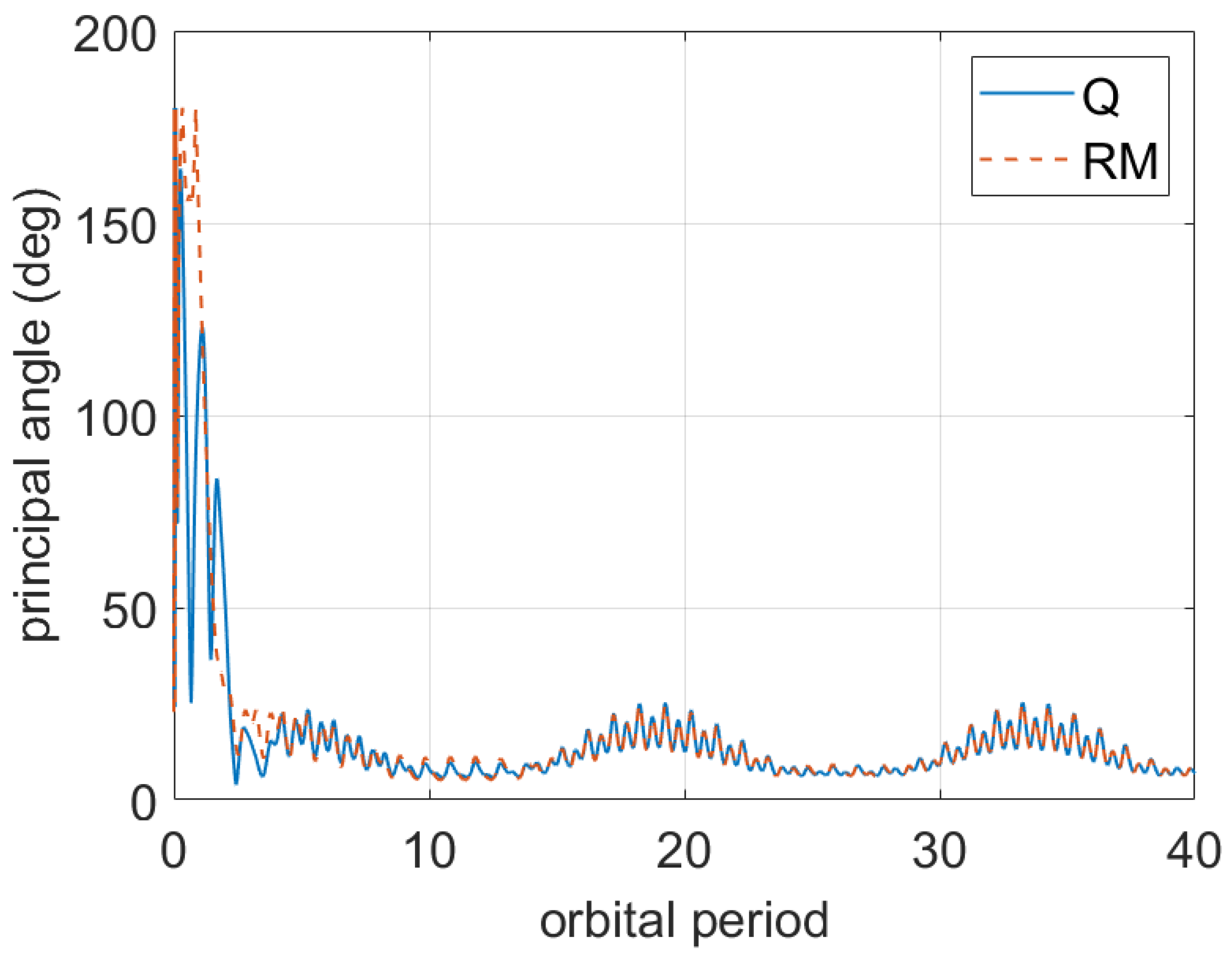
Figure 1 displays the time histories of the principal angle for a single run obtained by using quaternion feedback and rotation matrix feedback.
It turns out that, for this specific run, the settling time obtained with quaternion feedback is equal to 11 orbital periods, whereas by using rotation matrix feedback, the settling time is equal to 14 orbital periods. The value of is equal to 2.50 104 A2 m4 s for both control laws.
4.2. Perturbed Case
In this subsection, the performance comparison is carried out by considering a more realistic scenario in which the disturbance torques described in Section 2.4 act on the spacecraft and in which the inclined dipole model is adopted. Moreover, in this case the residual magnetic torque is approximately compensated by modifying the stabilizing laws in Equations (24) and (25) as follows.
The term represents an estimation of the residual dipole moment obtained by means of a Kalman filter, as reported in Appendix B.
In such a scenario, it is not appropriate to choose the settling time for the principal angle as the performance index that measures the speed of convergence. In fact, because of the presence of , the principal angle will not converge to 0. It will oscillate about some residual value. Thus, it more appropriate to select the Integral Time Absolute Error (ITAE) [19] as index for the speed of convergence for the principal angle, which is defined as follows.
In ITAE, the principal angle is weighted by time so that a high value of the principal angle at later times is penalized more than that at earlier times. In this perturbed case, is set equal to 40 so that the spacecraft’s attitude can reach a steady-state condition. On the other hand, index in Equation (27) is still used to measure the energy required to apply the control action.
A new Monte Carlo campaign including 100 runs has been executed. The initial rotation matrix , initial quaternion , initial angular velocity 20 deg/s, and initial argument of the spacecraft have been all randomly selected, as explained in the previous subsection.
The results of the campaign are reported in Table 5.
In the table, denotes the mean value of ITAE, and denotes the number of runs (expressed in percentage on the total number) in which .
The statistics show that in terms of both ITAE and energy consumption, quaternion feedback performs better than rotation matrix feedback.
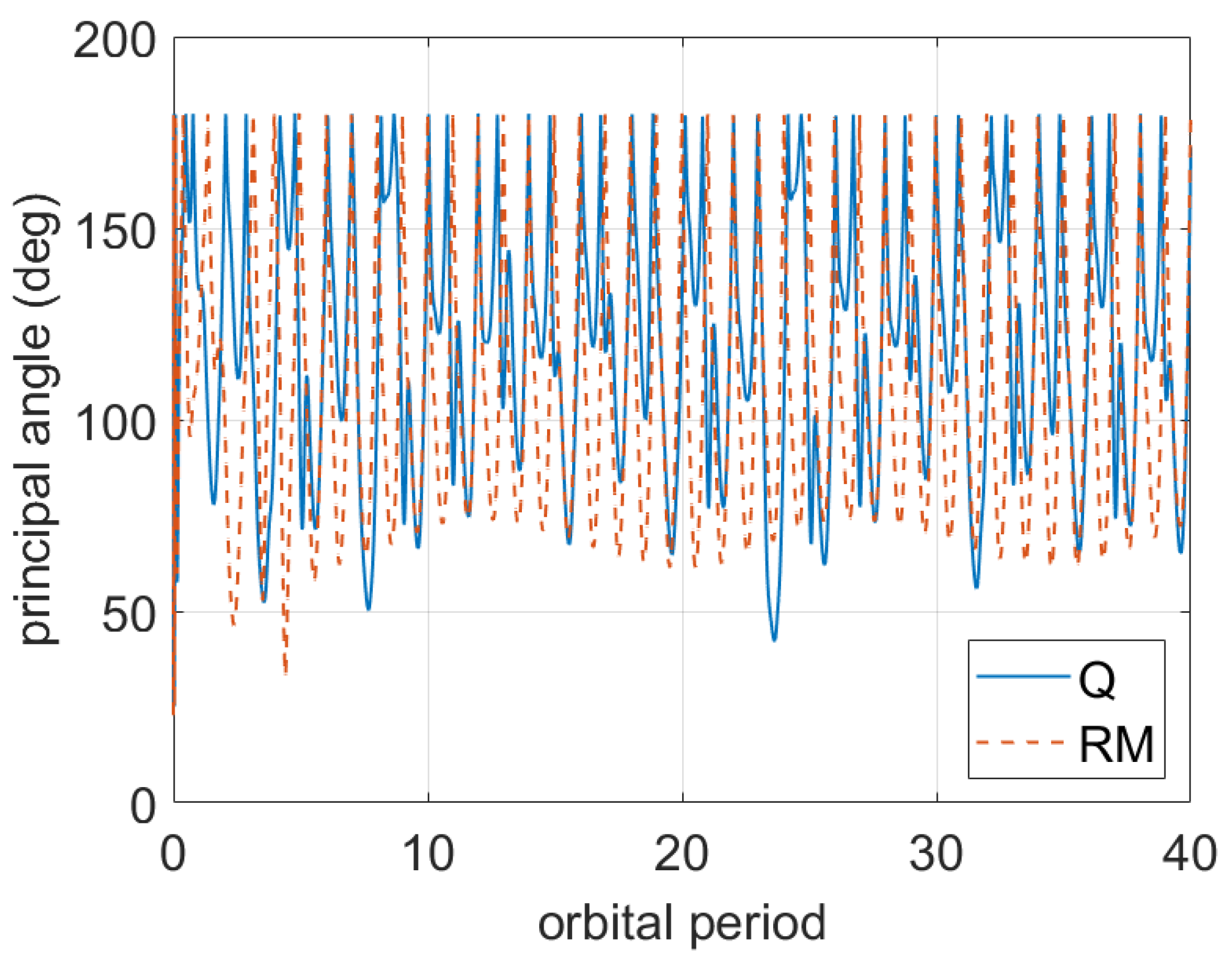
Figure 2 displays the time histories of the principal angle for a single run obtained by using quaternion feedback and rotation matrix feedback.
It turns out that for this specific run, the ITAE obtained with quaternion feedback is equal to 3.247 1011 deg sec, whereas the ITAE is equal to 3.255 1011 deg sec when using rotation matrix feedback. Moreover, the values of are, respectively, equal to 2.017 104 A2 m4 s and 2.062 104 A2 m4 s.
5. Conclusions
In this paper, a numerical comparison between quaternion plus attitude rate feedback and rotation matrix plus attitude rate feedback has been performed for a case study of an Earth-pointing spacecraft equipped with magnetorquers only as torque actuators. Monte Carlo campaigns show that in both nominal and perturbed conditions quaternion feedback achieves a faster convergence to the nominal attitude. Moreover, in terms of energy consumption, the two stabilizing laws are comparable in nominal conditions. However, quaternion feedback requires less energy in perturbed conditions. Note that, by using quaternion feedback, the unwinding phenomenon can occur, and its occurrence typically results in slower convergence and higher energy consumption. Thus, the fact that, in this study, quaternion feedback performs better both in terms of speed of convergence and of energy consumption testifies that the unwinding phenomenon most likely has occurred in rare simulation runs of Monte Carlo campaigns that have been executed.
Funding
This research received no external funding.
Conflicts of Interest
The author declare no conflict of interest.
Appendix A. Gain Selection
The goal of this appendix to present a method for determining effective values for the 3 × 3 matrix gains and . The method was obtained in [20] (see also [7]).
Let us neglect disturbance torque by setting , and consider the linear approximation of the closed-loop system given by Equations (1) and (14) and either (24) or (25). The linear approximation with either control laws is given by the following linear time-varying system:
which is subject to the state-feedback.
In the above equations, .
For selecting matrix gains and (or equivalently matrix gain K), consider the aligned dipole model of the geomagnetic field for which case is periodic with period (see Equation (22)). Then, matrix gain K is chosen so that the closed-loop system given by Equations (A1) and (A2) is asymptotically stable and control (A2) minimizes the following quadratic performance index:
where Q is a 6 × 6 positive semidefinite matrix, R is a 3 × 3 positive definite matrix, and the expectation operator is taken over the set of possible values for the initial state , which is assumed to be a random variable having zero mean and known covariance . Table A1 reports the values selected for those matrices as well as the initial guesses for and , respectively.

Table A1.
Parameters for gain selection.
| Q | R | |||
|---|---|---|---|---|
Appendix B. Compensation for the Residual Magnetic Torque
This appendix presents the method employed to compensate for the residual magnetic torque in Equation (23). The approach is based on obtaining an estimate of and plugging it into the stabilizing laws in Equation (28).
In order to estimate , we employ the method presented in [21], which uses a Kalman filter. Consider the following model of attitude dynamics:
which is obtained from Equations (7), (10), and (23) and in which the gravity gradient torque , aerodynamic torque , and solar radiation pressure torque are all neglected. In the above equation, is given by either of the stabilizing laws in Equation (28). Moreover, is modeled as constant. Thus, the following is the case.
Note that when the spacecraft attitude is in nominal conditions, and, consequently, (see Equations (5) and (6)). We introduce and determine the equation for , and we linearize it about , obtaining the following.
Note that in the linearized equation, the zero mean process noise has been added to take into account all the approximations that were introduced. Similarly, Equation (A5) is modified as follows:
where the zero mean process noise has been included to take into account possible time variations of the residual magnetic dipole moment.
Consider discrete times , where is the sampling interval, and integrate Equations (A6) and (A7) over interval . If is sufficiently small , , , , and can be approximately considered constant over the integration interval and are equal to , , , , and , respectively. Thus, the following equation is obtained:
where the following is the case.
Moreover, since can be measured, consider the following observation equation:
where is a zero mean measurement noise. Thus, the estimation of denoted by is obtained by designing a Kalman filter to estimate the state of Equation (A8) with observation Equation (A9) (see [22]).
The following data are employed to design the Kalman filter (see [12]). The sampling time is selected to s. The estimates are initialized to , . The corresponding covariance matrices are set to and . The covariance matrices of , , and v are chosen as , , and respectively.
In order to evaluate the performance of the proposed estimation method, the time histories of of obtained in the Monte Carlo campaign for the perturbed case using rotation matrix feedback are displayed in Figure A1. It is convenient to recall that, in the campaign, the residual magnetic dipole moment is constant and equal to (see Table 3). Similar time behaviors are obtained in the Monte Carlo campaign for the perturbed case using quaternion feedback and are not reported to save space. An important aspect shown in Figure A1 is that achieves steady state after few orbital periods.
Figure A1.
Time histories of obtained in the Monte Carlo campaign for the perturbed case using rotation matrix feedback.
Figure A1.
Time histories of obtained in the Monte Carlo campaign for the perturbed case using rotation matrix feedback.

In addition, Table A2 reports the statistics for obtained from the Monte Carlo campaign for the perturbed case using either quaternion feedback or rotation matrix feedback.
Table A2.
Statistics on from the Monte Carlo campaign for the perturbed case using either quaternion feedback (Q) or rotation matrix feedback (RM). In the campaign, the residual magnetic dipole moment is constant and equal to (see Table 3).
Table A2.
Statistics on from the Monte Carlo campaign for the perturbed case using either quaternion feedback (Q) or rotation matrix feedback (RM). In the campaign, the residual magnetic dipole moment is constant and equal to (see Table 3).
| Q | mean value (A m2) | standard deviation (A m2) |
| 0.14 | 0.75 | |
| −0.087 | 0.83 | |
| −0.11 | 0.78 | |
| RM | mean value (A m2) | standard deviation (A m2) |
| 0.18 | 0.83 | |
| −0.063 | 1.00 | |
| −0.13 | 0.88 |
The large standard deviations show that the estimation of is not accurate. Consequently, the compensation of the residual magnetic torque is not accurate either. Nevertheless, the proposed compensation is still highly beneficial. In fact, by running several simulations in perturbed conditions without operating any compensation of , it can be observed that no convergence to the nominal Earth-pointing attitude is achieved, as displayed in Figure A2, which is obtained from one of those simulations.
Figure A2.
Time histories of principal angle using quaternion feedback (Q, blue solid line) and using rotation matrix feedback (RM, red dashed line) obtained in a simulation in perturbed conditions without compensation of the residual magnetic torque.
Figure A2.
Time histories of principal angle using quaternion feedback (Q, blue solid line) and using rotation matrix feedback (RM, red dashed line) obtained in a simulation in perturbed conditions without compensation of the residual magnetic torque.

References
- Ovchinnikov, M.Y.; Roldugin, D. A survey on active magnetic attitude control algorithms for small satellites. Prog. Aerosp. Sci. 2019, 109, 100546. [Google Scholar] [CrossRef]
- Celani, F. Robust three-axis attitude stabilization for inertial pointing spacecraft using magnetorquers. Acta Astronaut. 2015, 107, 87–96. [Google Scholar] [CrossRef] [Green Version]
- Lovera, M.; Astolfi, A. Spacecraft attitude control using magnetic actuators. Automatica 2004, 40, 1405–1414. [Google Scholar] [CrossRef]
- Lovera, M.; Astolfi, A. Global magnetic attitude control of inertially pointing spacecraft. J. Guid. Control. Dyn. 2005, 28, 1065–1067. [Google Scholar] [CrossRef]
- Ovchinnikov, M.; Roldugin, D.; Penkov, V. Three-axis active magnetic attitude control asymptotical study. Acta Astronaut. 2015, 110, 279–286. [Google Scholar] [CrossRef]
- Wiśniewski, R.; Blanke, M. Fully magnetic attitude control for spacecraft subject to gravity gradient. Automatica 1999, 35, 1201–1214. [Google Scholar] [CrossRef]
- Celani, F. Gain Selection for Attitude Stabilization of Earth-Pointing Spacecraft Using Magnetorquers. Aerotec. Missili Spaz. 2021, 100, 15–24. [Google Scholar] [CrossRef]
- Ovchinnikov, M.; Roldugin, D.; Ivanov, D.; Penkov, V. Choosing control parameters for three axis magnetic stabilization in orbital frame. Acta Astronaut. 2015, 116, 74–77. [Google Scholar] [CrossRef]
- Psiaki, M.L. Magnetic Torquer Attitude Control via Asymptotic Periodic Linear Quadratic Regulation. J. Guid. Control. Dyn. 2001, 24, 386–394. [Google Scholar] [CrossRef]
- Yang, Y. An efficient algorithm for periodic Riccati equation with periodically time-varying input matrix. Automatica 2017, 78, 103–109. [Google Scholar] [CrossRef] [Green Version]
- Chaturvedi, N.A.; Sanyal, A.K.; McClamroch, N.H. Rigid-body attitude control. IEEE Control Syst. Mag. 2011, 31, 30–51. [Google Scholar]
- Avanzini, G.; de Angelis, E.L.; Giulietti, F. Two-timescale magnetic attitude control of Low-Earth-Orbit spacecraft. Aerosp. Sci. Technol. 2021, 116, 106884. [Google Scholar] [CrossRef]
- Sidi, M.J. Spacecraft Dynamics and Control; Cambridge University Press: Cambridge, MA, USA, 1997. [Google Scholar]
- Wie, B. Space Vehicle Dynamics and Control; American Institute of Aeronautics and Astronautics: Reston, VA, USA, 2008. [Google Scholar]
- de Ruiter, A.H.J.; Damaren, C.J.; Forbes, J.R. Spacecraft Dynamics and Control: An Introduction; Wiley: Chichester, UK, 2013. [Google Scholar]
- Wertz, J.R. (Ed.) Spacecraft Attitude Determination and Control; Kluwer Academic: Dordrecht, Holland, 1978. [Google Scholar]
- Alken, P.; Thébault, E.; Beggan, C.D.; Amit, H.; Aubert, J.; Baerenzung, J.; Bondar, T.; Brown, W.; Califf, S.; Chambodut, A.; et al. International geomagnetic reference field: The thirteenth generation. Earth Planets Space 2021, 73, 1–25. [Google Scholar] [CrossRef]
- Yakubovich, V.A.; Starzhinskii, V.M. Linear Differential Equations with Periodic Coefficients; J. Wiley & Sons: Jerusalem, Israel, 1975. [Google Scholar]
- Graham, D.; Lathrop, R.C. The synthesis of “optimum” transient response: Criteria and standard forms. Trans. Am. Inst. Electr. Eng. Part II Appl. Ind. 1953, 72, 273–288. [Google Scholar] [CrossRef] [Green Version]
- Viganò, L.; Bergamasco, M.; Lovera, M.; Varga, A. Optimal periodic output feedback control: A continuous-time approach and a case study. Int. J. Control 2010, 83, 897–914. [Google Scholar] [CrossRef]
- Inamori, T.; Sako, N.; Nakasuka, S. Magnetic dipole moment estimation and compensation for an accurate attitude control in nano-satellite missions. Acta Astronaut. 2011, 68, 2038–2046. [Google Scholar] [CrossRef]
- Anderson, B.D.; Moore, J.B. Optimal Filtering; Prentice-Hall: Englewood Cliffs, NJ, USA, 1979. [Google Scholar]
Figure 1.
Time histories of principal angle using quaternion feedback (Q, blue solid line) and using rotation matrix feedback (RM, red dashed line) (single run of the Monte Carlo campaign for the nominal case).
Figure 1.
Time histories of principal angle using quaternion feedback (Q, blue solid line) and using rotation matrix feedback (RM, red dashed line) (single run of the Monte Carlo campaign for the nominal case).

Figure 2.
Time histories of principal angle using quaternion feedback (Q, blue solid line) and using rotation matrix feedback (RM, red dashed line) (single run of the Monte Carlo campaign for the perturbed case).
Figure 2.
Time histories of principal angle using quaternion feedback (Q, blue solid line) and using rotation matrix feedback (RM, red dashed line) (single run of the Monte Carlo campaign for the perturbed case).

Table 1.
Notation.
| , , | vector of components of Eucledian vector with respect to frames , , and |
| respectively | |
| skew-symmetric matrix corresponding to (see Equation (2)) | |
| angular velocity of w.r.t. | |
| angular velocity of w.r.t. | |
| angular velocity of w.r.t. | |
| geomagnetic field at spacecraft | |
| q | quaternion representing rotation of w.r.t. |
| , | vector part and scalar part of q |
| vector from the Earth center to the satellite center of mass | |
| unit Eucledian vector corresponding to the -axis of | |
| identity matrix | |
| zero matrix |
Table 2.
Spacecraft, orbit, and geomagnetic field data.
| (kg m2) | (kg m2) | (km) | (deg) | (deg) | (Wb m) | (deg) |
| 1.416 | 2.0861 | 7021 | 98 | 137 | 7.71 1015 | 171 |
| (deg/day) | (Wb m) | (A m2) | ||||
| 360.99 | 7.60 1015 | 3.5 |
Table 3.
Disturbance torques data.
| (A m2) | (m) | (m2) | (kg/m3) | (W/m2) | |
| 2.2 | 0.22 | 6.39 10−13 | 1367 | ||
| (m) | (m2) | ||||
| 0.8 | 0.33 |
Table 4.
Statistics of the Monte Carlo campaign for the nominal case.
| control law | (orbital period) | (A2 m4 s) |
| Q | 13.8 | 6.20 104 |
| RM | 15.7 (+14%) | 6.19 104 (−0.1%) |
| 47% | 65% |
Table 5.
Statistics of the Monte Carlo campaign for the perturbed case.
| control law | (deg sec) | (A2 m4 sec) |
| Q | 1.3 1012 | 1.21 106 |
| RM | 2.1 1012 (+69%) | 1.36 10 6 (+12%) |
| 30% | 32% |
Publisher’s Note: MDPI stays neutral with regard to jurisdictional claims in published maps and institutional affiliations. |
© 2022 by the author. Licensee MDPI, Basel, Switzerland. This article is an open access article distributed under the terms and conditions of the Creative Commons Attribution (CC BY) license (https://creativecommons.org/licenses/by/4.0/).
Share and Cite
MDPI and ACS Style
Celani, F. Quaternion versus Rotation Matrix Feedback for Spacecraft Attitude Stabilization Using Magnetorquers. Aerospace 2022, 9, 24. https://doi.org/10.3390/aerospace9010024
AMA Style
Celani F. Quaternion versus Rotation Matrix Feedback for Spacecraft Attitude Stabilization Using Magnetorquers. Aerospace. 2022; 9(1):24. https://doi.org/10.3390/aerospace9010024
Chicago/Turabian StyleCelani, Fabio. 2022. "Quaternion versus Rotation Matrix Feedback for Spacecraft Attitude Stabilization Using Magnetorquers" Aerospace 9, no. 1: 24. https://doi.org/10.3390/aerospace9010024
Note that from the first issue of 2016, this journal uses article numbers instead of page numbers. See further details here.