Design Process and Environmental Impact of Unconventional Tail Airliners

Abstract

The future of aviation depends on reducing the environmental impact of the aircraft. Unconventional configurations can be the change the industry needs to achieve that goal. Therefore, the development of a tool that allows analyzing these configurations will contribute to their being considered more easily in future designs. This design procedure is based on an aerodynamic model and a weight methodology validated for unconventional tail designs. The load cases selected to size the structure were extracted from the certification regulations in force. In order to validate the methodology, the V-tail configuration was selected as a case study. The fuel savings reached with this tail configurations are around 0.7%, and the reduction in NO_x emissions are even greater. Thus, the methodology has been validated and it can be easily adapted to other unconventional tail configurations.

1. Introduction

At present, there is a growing awareness from most governments around the world about the emission of polluting gases into the atmosphere [1,2,3,4]. The environmental impact of aircraft rests on two main aspects: emission of noise and emission of particles and polluting gases that contribute to climate change [5,6,7]. On the other hand, the growth of air traffic is a continuum over the years. Despite the COVID-19 crisis, aviation is a resilient market, because it has recovered from similar downturns throughout its history, such as the Global Financial Crisis in 2008. In fact, both air traffic and aircraft deliveries are expected to recover to the previous annual growth levels, between 3% and 4%, for the next 20 years [8,9,10].

To enable this market development and the reduction of emissions, the performances of transport aircraft have been improving during over the past decades, especially, due to developments in key technology areas such as aerodynamics, propulsion, structures, avionics, materials, etc. [2,11,12]. Despite this clear evolution of jet aircraft throughout their history, their general configuration has hardly changed. Therefore, a field of study is opened in terms of the configuration of the aircraft concerned, being able to analyze unconventional configurations that potentially have benefits from the point of view of performances or emissions of polluting gases [13].

There are numerous studies that consider changes in airplane configuration and their impacts on performances. These novel configurations would result in a drastic change in the appearance of the airplane, for instance, joined-wing, flying wing, blended wing body or box-wing [14,15,16,17,18,19]. However, despite the potential benefits presented by these configurations, it is not foreseeable that manufacturers would launch these aircraft to market due to the drastic change they entail and their intrinsic complexity. In order to overcome these drawbacks, a small step in this direction would be to consider those novel configurations which suppose a minor change in the appearance of the aircraft. Thus, both manufacturers and airlines could evaluate in a more controlled way the impact of these solutions on their companies, in order to undertake a riskier project in the future. Precisely, in this context, unconventional tail configurations are solutions aligned to this idea.

Aircraft emissions can be divided into those which are proportional to fuel consumption and those which are not. Among species which belong to the first group are CO₂, H₂O and SO_x. Thus, just by using the respective emission index, it is possible to calculate them from the fuel flow data. On the other hand, for the other emission species (NO_x, CO, HC and soot), there are several methodologies to estimate them, such as P3T3, DLR and BFFM2, among others [20,21,22]. The use of unconventional tail configurations could reduce aircraft emissions through two main effects: reduction of aerodynamic drag and reduction of weight. Just the fuselage contributes around 28% to the parasite drag of the airplane and the empennage contributes 14% [23]. Regarding the weight, stabilizing surfaces could suppose around 5% of the maximum take off weight of the aircraft [16]. These percentages are indicative, but they show the possible repercussion that a new tail configuration could have.

In order to determine the potential benefits of unconventional tail configurations, a procedure to sizing these surfaces needs to be established for conceptual design stages. Classical methods to sizing tail surfaces at these initial steps of the aircraft design process are based on regressions built from the data available in the open literature. However, the available data related to unconventional tail configurations are not wide enough to build these design regressions because of their innovative nature. Thus, it is necessary to use design criteria based on the regulation in force to establish the feasible design for each tail configuration. A proposal of how to deal with the certification requirements to size an unconventional tail configuration has already been presented [24]. Thus, the next step is to analyze the impact of these novel tail configurations in weight and drag of the aircraft and, consequently, in fuel consumption and emissions of a given route. In the case of the drag, there are several methods to estimate it which are applicable to unconventional configurations [25,26,27,28]. However, the methods usually employed to estimate the weight of tail surfaces in conceptual design stages are empirical expressions based on statistical data and correction factors derived from designers’ experience. These kind of methods are not adequate for unconventional tail configurations as there are not enough data to build correlations. It is true that, for the simplest configurations, it is possible to adapt these empirical formulae, as is the case of V-tail configuration. However, there is no guarantee that the adaptation ends in reliable results if there is no other method to validate it.

In consequence, a methodology to estimate the weight of tail surfaces which is applicable to unconventional tail configurations is required. It needs to be fast to be used in early conceptual design stages but also reliable enough to reach results in the usual margin of error admissible in this phase of the design process, which is around 5–10% [16]. This weight method is going to be calibrated for a reference aircraft with conventional tail surfaces, which are formed by a horizontal surface, attached to the rear fuselage, and a vertical stabilizer. The weight estimation is performed by designing the tail structure attending to the loads that it needs to bear. These load cases are chosen from those described in the certification codes for commercial transport aircraft. Once the methodology is adjusted, it is the moment to apply it to an unconventional tail configuration. Thus, as indicated above, it is possible to establish a feasible design space based on the aircraft regulation in force so that, inside this feasible design space, an optimal solution can be found trying to minimize the weight of the tail surface, the drag and even the fuel consumption for a certain route. Optimization studies, from the standpoint of the weight and the drag, have already been presented in other previous studies, even a combination of them through MDO (Multidisciplinary Design Optimization) techniques [29]. Nevertheless, these approaches lose the point of view of the physics of the problem. It is not enough to build an artificial objective function as an arbitrary combination of drag and weight. It is better to analyze a useful combination of them, which is the equation that estimates the fuel consumption of the aircraft, including the effect of weight and drag. Thus, this is the final objective of this paper: determining a design procedure for unconventional tail design in order to analyze the potential fuel savings. The case study selected for demonstrating the methodology is the V-tail configuration, which is the simplest unconventional tail and has been deeply studied in the state of the art, so a comparison of the results which have been reached is feasible. The decision of selecting maneuvers included in certification codes, for sizing the structure and estimating the weight, is the most convenient approach to the problem, because the design must accomplish with the regulation in force if manufacturers want to develop the product. Therefore, the certification rules must be taken into account from the beginning of the research. This is a differentiated approach in V-tail configuration studies from those that can be found in the state of the art, because in this present case the objective is the commercial transport aviation sector, instead of other classical sectors where V-tail are more common, e.g., in unmanned aircraft [30,31,32].

The paper is organized so that it presents, as first step, the design strategy and the reference aircraft selected to perform the design. Then, a brief description of the aerodynamic model is included. The next step is to present the load cases selected and how they are considered in this study making use of the former aerodynamic model. After that, the weight estimation methodology is presented. Once all models have been explained, it is the moment to calibrate them for a reference aircraft with conventional tail configuration. Finally, the application of the methodology for the unconventional tail configuration selected is shown, analyzing the potential benefits or drawbacks of using the V-tail configuration instead of the conventional one for the chosen reference aircraft.

2. Materials and Methods

2.1. Design Strategy and Reference Aircraft

The objective is to design a V-tail that develops the same functions as a conventional tail configuration of a reference airplane, so that it is possible to substitute the original tail with the novel one. Four conditions are selected to assure that both configurations have the same functions. The first one is to guarantee that the static stability derivatives, both longitudinal and lateral, in cruise conditions are the same in both cases, or the unconventional tail aircraft would behave better statically. The second is controlling the aircraft after critical engine failure during climb in the second segment. For doing that, the tail control must cancel the yaw moment generated by the unbalanced thrust with a bank angle lower than 5${}^{\circ }$. The third condition is to allow the aircraft adequate control in crosswind landing conditions. To do that, the tail control must cancel the yaw moment generated by the crosswind with a bank angle lower than 5${}^{\circ }$. Finally, the fourth is allowing the trim of the aircraft in any other condition. Of course, it is possible to select much more stringent conditions that constraint the design space of the unconventional tail. The authors selected these as a first approximation to the problems because they can be modeled in a simple, but accurate enough, way in order to accomplish with the necessities of the conceptual design stages. The solution of the feasible design space for V-tail configurations taking into account these conditions has already been performed [24].

The structure is sized in order to bear the load cases presented in Section 2.3 and, consequently, the tail weight is estimated. In order to undertake a viability study of a novel configuration, the main parameter that needs to be analyzed is the fuel consumption of the aircraft. Thus, the final objective function to be optimized is the fuel weight for a given mission, which measures interactions between weight and drag. Once this solution is determined, the final step is to compare the original configuration with the unconventional one in terms of fuel consumption for a certain route. In order to perform this comparative study, it is necessary to choose a reference aircraft.

The reference aircraft has been selected from the database CeRAS (Central Reference Aircraft data System). This database had the objective of harboring design data of commercial transport aircraft. This idea was born because the scientific community found problems and inconsistencies in airplane data available in the open literature. Thus, this project tried to harmonize the sources of information in order to allow extracting better conclusions into comparative studies. This database was built in RWTH Aachen University, with Airbus collaboration [33]. The only available information in the database corresponds to a short-range aircraft denominated CSR-01. The most important parameters that described this aircraft are included in

Table 1. CSR-01 parameters available on CeRAS database.

Variable	Value
Maximum take of weight	77,000 kg
Operating empty weight	42,100 kg
Number of passengers	150
Mach number	0.78
Wing area	122.41 m2
Horizontal tail area	32.23 m2
Vertical tail area	28.21 m2
Horizontal tail weight	682 kg
Vertical tail weight	522 kg

. The database also includes information about greenhouse emissions of the aircraft in a certain route.

The database contains a three-views drawing, and a detailed description of the planform wing geometry. With this information and some design recommendations included in the open literature [25,28,34], it is possible to determine the characteristics of the high-lift devices. Additionally, the database includes information about the drag polar of the airplane depending on the Mach number and the flight configuration, represented in Figure 1. Even though the database does not indicate explicitly the Mach number at which the drag polar curves of take-off, climbing, approach and approach with extended landing gear have been calculated, the average speed in the design route for the two first conditions are around 0.25 Mach and for the two last are around 0.2 Mach.

From the standpoint of the tail surfaces, the geometries are fully defined in the database. However, some parameters need to be estimated. For instance, the maximum control deflections have been taken from Sanchez-Carmona and Cuerno-Rejado [24]; the percentage of chord that the controls take up is considered as 25%, according to the state of the art of other airplanes; and the airfoils for the tail surfaces selected are NACA 0012 in the case of the horizontal tailplane and NACA 0009 for the vertical tailplane. Once these tail parameters are known, it is possible to estimate the contributions of the tails to the zero-lift drag coefficient of the airplane. To perform this, the method proposed in [25] was followed, which is the same for horizontal and vertical surfaces:

$$c_{D0}{S}_w=2c_F\left(1+2.75(t/c)co{s}^2{\Lambda }_{0.5}\right)S.$$

(1)

In Equation (1), $c_{D0}$ is the zero-lift drag coefficient, $S_w$ is the wing area, S represents the wetted area of each stabilizer, $c_F$ is the friction coefficient that depends on the Reynolds number based on the mean geometric chord of each surface, $t/c$ is the relative thickness and ${\Lambda }_{0.5}$ is the sweep angle of the mean chords line. Following this methodology, the resultant zero-lift drag coefficients of the stabilizers are 0.0014 for the vertical surface and 0.0019 for the horizontal one. From the structural standpoint, it is necessary to know how the torsion box is defined according to the airfoils installed in each tail surface. The torsion box cross section is supposed as rectangular. Thus, the necessary hypotheses are to fix the position of the front and rear spars. In both cases, horizontal and vertical tail planes, it was decided to fix the front spar at 15% of the chord and the rear one to 55%. Furthermore, it is supposed that the ribs are separated from one to the following by 1 m, according to other analogous structures analyzed. The distance between the vertical stiffeners of the spars is 0.5 m. In order to determine the weight of the secondary and miscellaneous structures, it is necessary to know the values of geometrical magnitudes such as the fixed leading edge area, fixed trailed edge area or the area of tail control surfaces. All these magnitudes, which depend on the aircraft geometry, can be found in [35], which uses this same aircraft for its study.

The route selected for this study is defined as the design route in CeRAS database. The mission consists in transporting 13,608 kg of payload 5093 km, with a Mach number of 0.78 and an altitude of 35,000 ft. The database indicates that this mission is performed with a takeoff weight of 74,102 kg, which is slightly lower than the maximum takeoff weight. Furthermore, the reserve fuel is 3258 kg and the trip fuel is 14,992 kg, removing the fuel consumed during the taxi previous to takeoff and that after landing. At this point, it is necessary to adjust a model so that it can estimate with enough accuracy the trip fuel. This model is used for predicting the fuel consumption of the redesigned aircraft. The fuel required during the trip is estimated as the one burned for takeoff, climb, descent and landing, in addition to that required for the cruise phase [36]. The fuel burned during cruise phase can be estimated using Breguet range equation. The fuel required for the other phases is around 4% of the takeoff weight. The cruise starts at around 97.5% of takeoff weight, and the distance considered for Breguet range equation is obtained shortening the actual range by the distance traveled during the climb and descent phases, which is around 300 km. Keeping in mind these typical values, they can be slightly modified in order to better adjust the model to this specific aircraft in this specific route. Thus, the trip fuel, $TF$, is estimated as follows:

$$TF=TOW\left[0.037+0.98\left(1-e^{-\frac{R-370.4}{K}}\right)\right],$$

(2)

where R is the range and K is the Breguet range parameter, while the takeoff weight, $TOW$, is the addition of the landing weight, $LW$, to the trip fuel:

$$TOW=TF+LW.$$

(3)

The Breguet range parameter is calculated following the next expression in the case of turbofan aircraft [37]:

$$K=\frac{V}{c_e}\frac{c_L}{c_D}.$$

(4)

In Equation (4) appears the cruise speed V, the specific fuel consumption in cruise conditions $c_e$ and the aerodynamic efficiency in cruising conditions $c_L/c_D$. The specific fuel consumption is included in the database and takes the value 16.03 mg/Ns. The aerodynamic efficiency corresponds to the average along the trip, and it is possible to estimate it as the one corresponding to the point where the aircraft has consumed a half of the trip fuel. In that point, the airplane weight is the average between the takeoff and landing weights. Balancing the vertical forces of the aircraft in cruising conditions and by means of the drag polar, it is possible to determine the aerodynamic efficiency. It is remarkable that this procedure to determine the takeoff weight for the design route is iterative because the Breguet range parameter depends on the takeoff weight, through the aerodynamic efficiency. Once the procedure converges, the result is that the Breguet range parameter is 25,613.97 km, the takeoff weight is 73,896.84 kg and the trip fuel is 14,927.85 kg. These results present an error of $-0.277$% in the case of the takeoff weight and $-0.428$% in the case of the fuel consumption, when compared with the values contained in the database. These errors are associated with the limitations of the chosen model to estimate the trip fuel, which is based on supposing that the cruise phase of the flight is performed with a constant range parameter. This hypothesis implies that specific fuel consumption, speed and aerodynamic efficiency are constant along the cruise phase. According to Risse et al. [33], the first two magnitudes can be considered as constant, but not the aerodynamic efficiency, because the lift coefficient needs to vary to balance the variations in aircraft weight along the flight. Despite the hypotheses on which this model is based, the results are accurate enough for this study. Thus, it is possible to conclude that the proposed method is validated and calibrated for the reference aircraft and the given route.

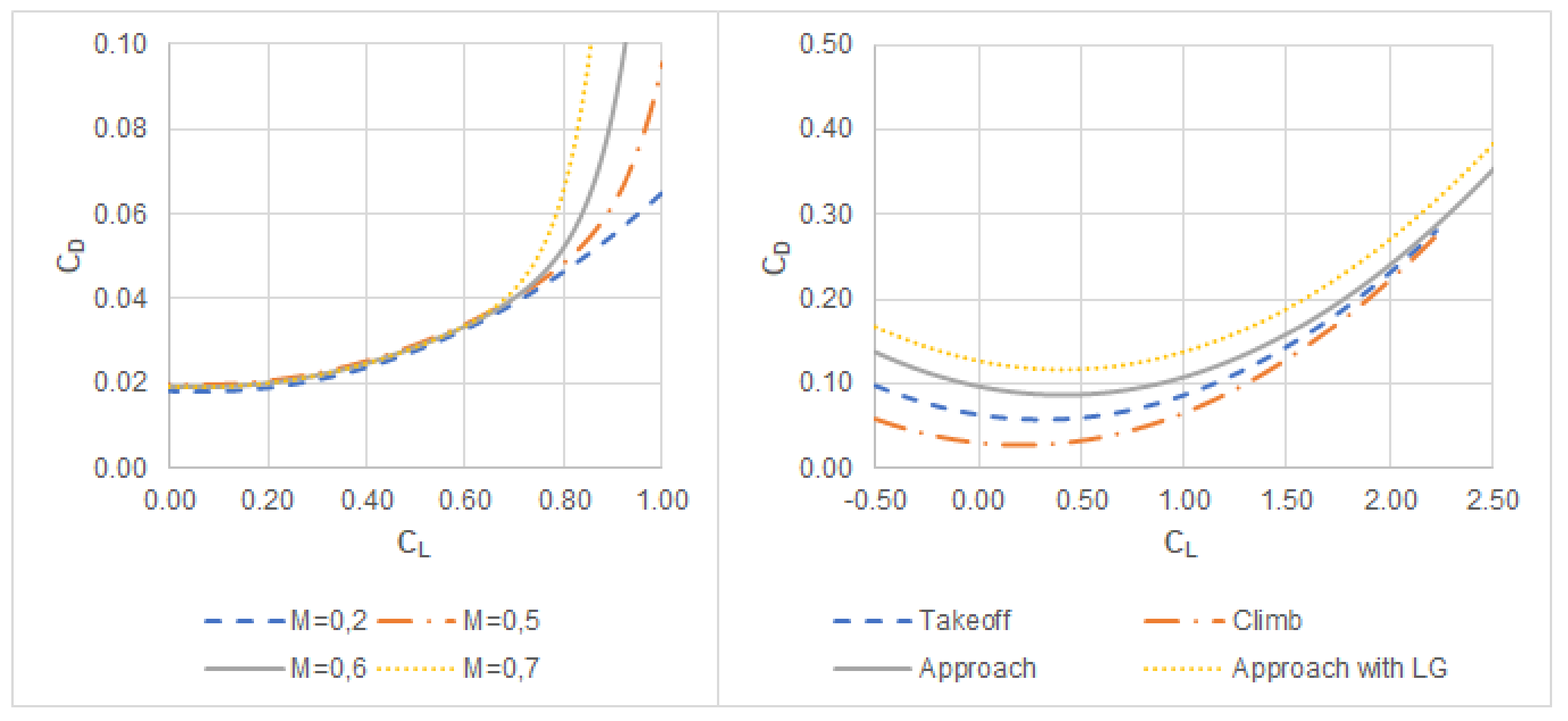
2.2. Aerodynamic Model

The aerodynamic model used in this study in order to estimate the stability derivatives and the aerodynamic loads is a combination of semi-empirical methods and VLM (Vortex Lattice Method). This technique was validated for unconventional tail configurations, using as a reference case V-tail [24]. The idea is to employ classical semi-empirical methods to determine the contributions of all the airplane to the stability derivatives and aerodynamic forces except the contributions of the tail surfaces, which are considered by means of an improved version of Tornado software. Tornado is a tool based on linear aerodynamics though for conceptual design applications [38]. It allows calculating both stability derivatives and forces distribution along the surface’s span. In addition, the software includes the Prandt-Glauert correction in order to expand the validity of its results to high subsonic regime [39]. Despite the wide versatility of the software, there are some inaccuracies that need to be solved in order to analyze results for unconventional tails. Among them, there are the non-linearities of controls deflections and interaction between surfaces and fuselage. Therefore, it is proposed to analyze the surfaces separately, calculating the aerodynamic forces of the isolated tail with Tornado, including the controls corrections, and the rest elements of the aircraft with semi-empirical methodologies. This decision is based on the reasoning that the classical semi-empirical techniques are not valid for unconventional geometries, so it is not possible to model the full aircraft through these methods. On the other hand, the versatility of Tornado can be used for considering these novel configurations.

It is noticeable that the cruise condition selected previously, for determining the fuel consumption, is not possible to be chosen in order to perform the cruise stability study. It is because the Mach number is within the high subsonic regime and exceeds the validity of the aerodynamic model selected. Because of that, it is necessary to select other cruise condition for calculating the stability performance. Despite that, if the novel aircraft design has the same stability characteristics in this other cruise condition, it is expected that it also develops the same behavior in any other cruise condition. Thus, the flight condition selected for these estimations is Mach 0.6 and an altitude of 22,000 ft. This combination corresponds to the design maneuvering speed for the chosen altitude at maximum takeoff weight, which is an advantage because several of the load cases considered in this study must be studied for this speed, as explained in the next section.

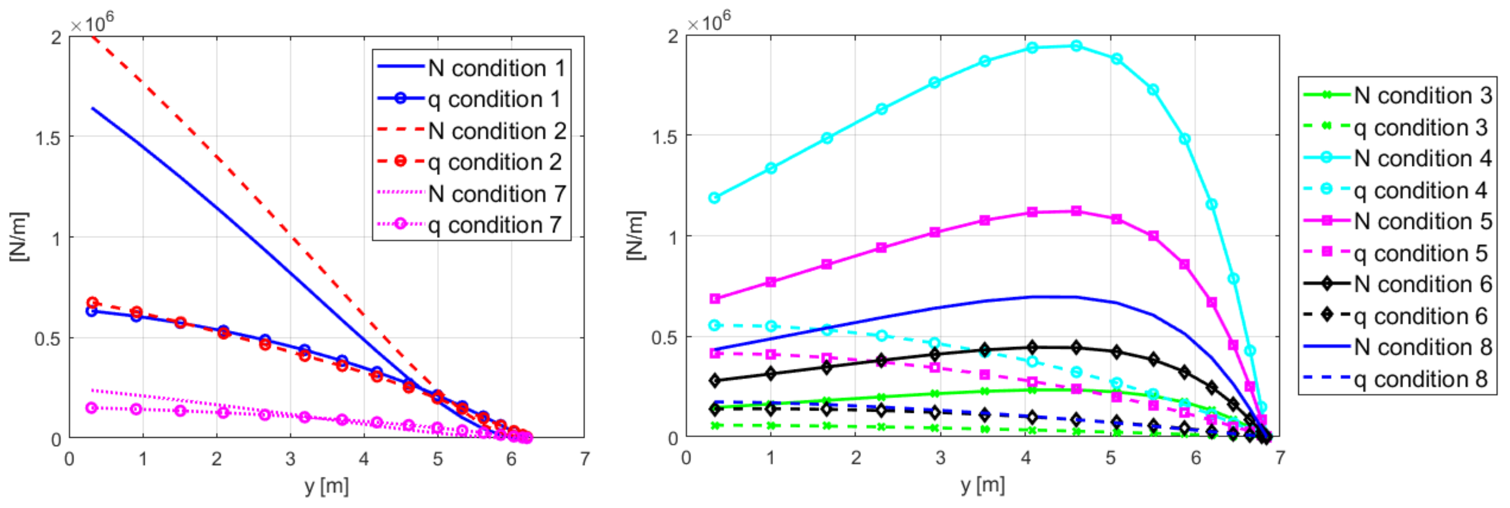
2.3. Load Cases for Tails Design

The load cases selected to size the structure were extracted from the current regulation codes for airplanes certification. The regulations in force in the European Union [40] (CS-25) and United States of America [41] (FAR-25) applicable to large airplanes are divided into different subparts. In both cases, Subpart C deals with the structural requirements of the aircraft that obtains its airworthiness certification through these regulations. In general, aircraft load analyses are very complex and require advanced tools to perform them, because there is a coupling between the motion of the aircraft, the aerodynamic forces and the deformations of the structure. Thus, a series of simplified models are presented in order to allow designers to evaluate the loads of tail surfaces in early stages of aircraft design [42]. The load cases can be separated into those which are related to the horizontal tail and those which affect the vertical tail.

Regarding the horizontal tail, the main conditions which need to be analyzed are the following: balanced maneuvers, unchecked elevator conditions, checked maneuvers and vertical gusts. It is true that there are other conditions such as rolling maneuvers or stalling that are included in the regulation, but the authors decided to leave them out of this study, to be considered in future works. From the standpoint of vertical tail loads, those considered in this study are: yawing maneuvers, rudder maneuvers, engine-out conditions and lateral gusts. Again, some other conditions exist that should be contemplated in order to broaden the study presented in this paper, for example a dynamic analysis caused by the presence of a lateral gust. The reason some maneuvers are not considered in this work, for both the horizontal tail design and the vertical surface one, is because the boundaries of the selected aerodynamic tool are exceeded.

2.3.1. Symmetric Maneuvers

The symmetric maneuvers are those that introduce loads into the horizontal tail. One type of these maneuvers considers that the pitching acceleration is equal to zero. The equations to be solved to determine the horizontal tail loads in these conditions are pitching moment balancing and vertical forces equilibrium. The solution of this system of equations ends in the angle of attack and the deflection of the elevator needed to balance the aircraft.

The other type of maneuvers that are considered as symmetric are those due to deflect the elevator in a rapid way. Among these maneuvers, there are two categories: unchecked and checked deflections. Unchecked deflections suppose that the movement of the elevator is sudden, producing maximum positive pitch acceleration of the aircraft when it is flying in cruise and stationary flight at design maneuvering speed $V_A$ [40,41]. The dynamic response of the aircraft must be taken into account for the determination of the resultant tail loads. Nevertheless, if the center of gravity suffers a vertical acceleration which supposes that the positive limit maneuvering load factor is exceeded during the dynamic response of the aircraft after the unchecked deflection, the loads that appear after reaching this load factor must not be considered. In order to reach this maximum acceleration, the elevator must be deflected from the position that balances the aircraft in horizontal stationary cruise flight, which is the solution of the previous system of equations, to the maximum position, staying at that position after that. The sudden deflection can be modeled through lineal or exponential laws. On the other hand, the checked deflection consists in reaching the maximum deflection of the elevator, but, after that, the elevators return to the balanced position. This law is modeled through a sinusoid that achieves these conditions. The characteristics of that sinusoid can be found in the regulation in force, in article CS 25.33137. In the case of the USA regulations, the code indicates that this maneuver must not exceed the limit loads, neither positive nor negative. The details of this maneuver are collected in article FAR 25.33138.

In order to model the loads generated in the horizontal tail after a maneuver with pitching acceleration caused by an unchecked deflection of the elevator, there is a simplified model that does not imply solving the dynamic behavior of the aircraft. The increment of tail load and pitch movement of the aircraft caused by a sudden deflection of the elevator can be divided into two contributions: the change of the angle of attack and the change of the elevator deflection itself. This model can be found completely expanded in [42], but the final expression reached is the following:

$$L_t=L_{t,n=1}+k_r{L}_{t{\delta }_e}\Delta {\delta }_{emax}.$$

(5)

The first term of Equation (5), $L_{t,n=1}$, corresponds to the force generated by the tail for balancing the aircraft at cruise flight. $L_{t{\delta }_e}$ is the derivative of the tail force depending on the deflection of the elevator, ${\delta }_e$, and $\Delta {\delta }_{emax}$ is the increment of elevator deflection. The second term of Equation (5) corresponds to the increment of force produced by the increment of deflection between the balanced position and the maximum one. This last contribution must be reduced by a response factor, $k_r$, which is supposed to be 0.9, to be conservative in the result. This parameter should be used only when the critical combination of speed and altitude is reached, in terms of load. In this study, the loads are estimated through Tornado software. It does not allow a temporal law for controls input. Thus, the simplified model is perfect to perform an estimation of the loads generated by the unchecked maneuver. Therefore, for determining the loads, it is enough to balance the aircraft in the corresponding condition and, after that, deflect the elevator to the maximum position. Since, at this point, it is not clear which is the most critical case in terms of load, it is decided not to include the response factor, so the results are even more conservative. In the case of checked maneuvers, it is also possible to use a simplified model for estimating the load generated at the tail. Again, the work of Lomax [42] includes the whole deduction, but the final expression is:

$$L_t=L_{t,bal}+L_{t{\delta }_e}\Delta {\delta }_{ecm}.$$

(6)

The tail force necessary to balance the aircraft at a certain load factor, in the general case different from one, corresponds to the first term of the previous expression $L_{t,bal}$·$L_{t{\delta }_e}$ is the incremental tail load due to elevator and $\Delta {\delta }_{ecm}$ is the incremental check maneuver elevator angle. The second one represents the increment of force generated at the tail caused by the fact of increasing the elevator deflection from the balanced position in a value equal to:

$$\Delta {\delta }_{ecm}=-\left(1+CBF\right)\left({\delta }_{ebal}-{\delta }_{etrim}\right)$$

(7)

where $CBF$ is the checkback factor [42] that takes zero value when the control comes back to the balanced position and 0.5 for overcheck conditions; ${\delta }_{ebal}$ corresponds to the elevator angle deflection for balancing the aircraft in the general case of load factor considered to study; and ${\delta }_{etrim}$ is the angle that balances the aircraft for load factor equal to 1, that is, at the beginning of the maneuver.

Through this simplified model, it is possible to estimate the loads generated in the tail by means of Tornado software. Nevertheless, the code states that this maneuver must be studied for speeds from $V_A$ to $V_D$ (design diving speed), so the validity boundaries of the aerodynamic model would be exceeded. Thus, this load case will only be considered in this study for speeds where the aerodynamic model has enough accuracy, inside the range that the regulation in force indicates.

2.3.2. Gusts Loads

Airplanes fly in a fluid that presents turbulence in form of gusts that introduce loads into the aircraft and, consequently, in both stabilizers. The model chosen for estimating these forces starts from Pratt Criteria [43,44], which supposes a sinusoidal gust with semi-wavelength of 12.5 mean geometric chord and an attenuation factor, $K_g$, in relation with the instant equivalent gust. From the year 2000, both European and North American codes changed, and the new model for calculating the load factors in presence of gusts is more complicated and less intuitive. Thus, it has been decided to follow the older model in order to allow a better integration in this study, keeping more conservative results. Therefore, the angle of attack induced in the aircraft by a vertical gust and the tail load are [42]:

$$\Delta {\alpha }_w=\frac{180K_g{U}_{max}}{1.69V\pi },$$

(8)

$$L_t=L_{t,n=1}+\left(1-\frac{dϵ}{d\alpha }\right)\Delta {\alpha }_w{L}_{t\alpha }.$$

(9)

In Equation (8), $K_g$ is the gust alleviation factor, V is the aircraft speed and $U_{max}$ is the maximum gust speed. In Equation (9), $L_{t,n=1}$ is the tail force when load factor is one, $ϵ$ is the downwash angle, $\alpha$ is the angle of attack, $\Delta {\alpha }_w$ is the increment of angle of attack of the wing and $L_{t\alpha }$ is the increment of tail force due to the angle of attack.

In order to incorporate this model in the improved Tornado tool, the first step is to balance the aircraft in certain condition and, after that, to introduce the increment of angle of attack indicated in the former expression. This same model can be used for estimating the loads generated in the vertical tail if a lateral gust appears, just substituting the mass parameter as the corresponding aircraft certification code indicates [40,42].

2.3.3. Asymmetric Maneuvers

The aircraft must be designed to bear the loads resulting in the yaw maneuvers that are indicated between $V_{MC}$ (minimum control speed) and $V_D$ speeds, both included, according to the articles CS 25.35137 or FAR 25.35138. The aerodynamic moment generated around the center of gravity must be balanced in a conservative way. In addition, it must be considered that the yaw speed is equal to zero and the wings are level, because these hypotheses are conservative in the loads generated. The asymmetric maneuvers that affects to the vertical tail which are caused by the deflection of the rudder can be reduced to three conditions. The first maneuver, called Maneuver 1, with the airplane in flight without acceleration or yawing, considers that the rudder is deflected quickly to the maximum angle or until the deflection that supposes a pedal force equal to 1335 N. The second condition, Maneuver 2, with the rudder in the maximum position or the corresponding position to where the pilot has to make 1335 N in the pedal, considers that the aircraft turns around the z-axis, yawing movement, until the resulting steady sideslip angle. The third one, Maneuver 3, with the aircraft balanced in yaw at the previous rudder position, supposes that the control comes back to zero.

Maneuver 1 can easily be modeled through Tornado, because indicating the maximum rudder deflection is enough to estimate the resultant forces. Maneuver 2 can be simplified following the steps indicated in [42], where the loads can be estimated as the addition of the loads caused by the fact of the maximum rudder position and the loads generated by the resultant sideslip angle. Finally, in the case of Maneuver 3, it is possible to determine the loads subtracting the loads corresponding to the stationary sideslip angle with maximum deflection of the rudder and the condition of stationary sideslip angle with null rudder deflection. That means that the loads can be estimated by the ones caused by flying with the stationary sideslip angle.

Another asymmetrical maneuver that must be taken into account according to the code is the control of the aircraft after the failure of the critical engine, included in the articles FAR 25.36738 or CS 25.36737. The equations necessary to solve this problem are included in [24], and the final expression where the tail load is possible to be determined, is:

$$\frac{1}{2}\rho V^2{S}_{w}b{c}_{n_{A-T}}-\frac{1}{2}\rho V^2{S}_w{L}_{TV}{c}_{YT}+T_e{y}_e=0$$

(10)

In Equation (10), b is the wing span, $T_e$ is the thrust of the critical engine, $y_e$ is the lateral position of the critical engine, $c_{n_{A-T}}$ is the yawing moment coefficient of the aircraft neglecting the contribution of the tail, $L_{TV}$ is the tail moment arm and $c_{YT}$ is the lateral force coefficient of the tail, through which it is possible to determine the force generated in the vertical tail. The regulation establishes two conditions to be taken into account: the rudder deflection needed to balance the yaw moment generated by the asymmetry of thrust flying with zero sideslip angle and the sideslip angle needed to cancel the yaw moment without any deflection of the rudder. Maneuver 2, Maneuver 3 and controlling the aircraft after critical engine failure without deflection of the rudder can result in a sideslip angle over the validity boundary of Tornado software, which is around 10º. Because of that, it has been decided to substitute these conditions by the boundary sideslip angle of 10º, instead of determining the corresponding stationary angle in each case. This simplification is imposed by the range of validity of the aerodynamic model and should be modified in future works.

2.4. Weight Estimation Models

The weight estimation of an element of an aircraft can be carried out through different strategies [45]. In these early stages of the design process, it is desirable to use a method with enough accuracy but that allows the user to make sensitivity studies for variations of the design parameters. From the standpoint of accuracy, it is desirable to incorporate complex methods based on FEM (Finite Elements Method) that estimate the weight with around 1–2%. However, the accuracy of these methods depends on the level of knowledge of the structural geometry, which is fully unknown at this point of the design process. Thus, it is necessary to use a tool to estimate the structural weight which does not need a deep knowledge of the geometry, but capable of sizing the structure, performing sensitivity studies of design parameters in a relatively short time. Taking into account these necessities, there are two possible kinds of methodologies: statistical methods and quasi-analytical methods. In this paper, a combination of both methods is proposed to estimate the weight of the different elements that form the tail structure. These elements can be classified in the following main groups: torsion box, ribs and secondary and miscellaneous structure. Adding the contributions of the three groups, the whole mass of the tail can be estimated.

Statistical methods are based on the knowledge of data about conventional tail configurations. These methods are adequate to estimate the mass of those elements for which sizing is more difficult to be determined in this early stage of the design, for instance, the ribs or the secondary and miscellaneous structure. In [35], it is possible to find an application of these methodologies for estimating the weight of ribs and the elements that form part of the secondary and miscellaneous structure, such as controls, leading and trailing edges structure or joints. The methodology presented in the reference is an adaptation of a method thought for determining wing masses. In addition, a case study for unconventional tail configuration is performed, so its use for this paper is fully justified.

After this, the most important contributions to the tail mass are the mass corresponding to the torsion box, whose elements are spars, skin and stringers. Sanchez-Carmona et al. [35] presented a method to estimate the weight of the torsion box. They indicated that the method is based on classical methodologies developed for metallic elements and, after sizing them, the results are corrected by a factor corresponding to the quotient between the densities of usual material composites and typical aluminum alloys employed in aeronautical structures.

The selected procedure for sizing the structure depends on the value of a factor called Farrar’s factor. It was decided to take the maximum value of this factor because it ends into a lighter structure [46]. In order to incorporate this method into the weight estimation of a tail surface, some hypotheses were made:

• the torsion box bears bending, shear and torsion;
• the torsion box is approximated by a rectangular geometry, as shown in Figure 2;
• the stringers have Z-shape section, and the relation between width and height is a factor of 0.3;
• the spars are stiffened by vertical elements located every certain distance;
• the caps define the extremes of the spars, and their areas are neglected when comparing to total panel area;
• for each section, extrados and intrados panels have the same geometry (this consideration is taken because the tail surface could generate lift upwards or downwards, depending on the flight condition of the aircraft); and
• the panel is sized for a uniform shear load, corresponding to the maximum that appears in the panel.

Keeping these hypotheses in mind, a bending moment, $M_f$, generates a compression load per unit of length, N, equal to $M_f/h_t{b}_t$. The sign of the bending moment determines which element of the torsion box, intrados or extrados panels, is subjected to compression and, consequently, which panel is sized with the proposed methodology. Because both panels have the same geometry, it is irrelevant to retain the sign of the bending moment.

A torsion moment, $M_{Tor}$, generates a shear flux, $q_T$, equal to $M_{Tor}/2h_t{b}_t$, while a shear force, $F_c$, generates a maximum shear flux equal to $F_c/2h_t$. Because of the sign of the shear flux generated by the torsion moment and by the shear force could not be the same, the corresponding shear flux used for sizing the panel is $\left|q_T\right|+\left|F_c/2h_t\right|$, which is the highest possible and the most conservative one.

Among the load cases considered in Section 2.3, the most critical combinations of shear and compression loads were selected for each section of the surface. For this critical case, the corresponding torsion box will be sized. After that, it is possible to estimate the tail weight, adding the corresponding weight of the ribs and secondary and miscellaneous structures.

2.5. Emissions Models

The emissions of greenhouse gases can be estimated through different procedures depending on the species. In this context, emission index (EI) is defined as the mass of pollutant, in grams, divided by the mass of fuel used in kilograms [21]. As explained in the Introduction, emissions can be classified between those gases that are proportional to fuel consumption and those which are not. Therefore, for gases belonging to the first group, the emission indexes are constant. In this case, they can be directly calculated from the fuel weight consumption. The species which belong to this group are CO₂, H₂O and SO_x. The corresponding emission indices for them are: EI CO₂, 3149; EI H₂O, 1200; and EI SO_x, 0.84 [33].

On the other hand, NO_x, CO and HC emissions do not have constant emission indexes. At this point of conceptual design stage, several techniques can be applied in order to estimate these indexes. For this purpose, the ICAO Engine Emissions Databank [47] is a repository with information on exhaust emissions of those engines that have entered production. The information is based on experimental tests for an idealized landing/take-off cycle (LTO) in International Standard Atmosphere (ISA) conditions. The LTO cycle only assesses the emissions below 915 m (3000 ft) and, therefore, may not be a good guide for analyzing other flight modes, for instance, cruise [21]. The ICAO Databank includes information about the following phases of flight: take off, climb out, approach and taxi/ground idle. These conditions correspond to a throttle setting, in percent of maximum rated output, of 100%, 85%, 30% and 7%, respectively, to the four previous conditions. Nevertheless, there are several correction procedures to take into account altitude effects and estimate emissions in cruise conditions. Among them, Fuel Flow Method 2, developed by Boeing, and DLR (Deutsches Zentrum für Luft- und Raumfahrt e.V., literally German Center for Air- and Space-flight) method are simple methods that provide around 10% accuracy, which are adequate to use in these early stages of aircraft design with reduced available data [48].

Boeing’s Fuel Flow Method 2 (BFFM2) [49] is an empirical procedure which computes in-flight aircraft emissions using, as a base, the measured fuel flow and the engine ICAO data sheets. This method takes into account ambient pressure, temperature, humidity and Mach number. It enables the calculation of NO_x, CO and HC emissions [50]. DLR method is based on the same principle as BFFM2, but the way the parameters are manipulated and the required input data are different. The corresponding inputs in this case are total pressure and temperature which comprehend stagnation and flight speed effects. Furthermore, this methodology just enables the calculation of NO_x [48]. In this study, both methods are considered in order to check both paths.

The estimation of these emission indexes depends on ambient conditions and flight phases, since fuel flow changes. Because this study is undertaken by means of a comparison with a reference aircraft, emissions should be focused on the cruise flight. It is assume that emissions throughout the other phases are very similar in both CSR-01 and the redesigned aircraft. Thus, it is considered that all the fuel has been burnt during cruise phase. The uncertainties associated with this assumption are made in both aircraft, and they are neglected when a comparison between emissions is carried out.

3. Results

3.1. Test Case for Conventional Tail Configuration

This section allows calibrating the methodologies presented previously in order to extract more relevant conclusions when the results for the unconventional tail are performed. The weight estimation method exposed in previous section needs to know the loads generated in the tail surfaces. Keeping in mind the limitations of the aerodynamic model, the following maneuvers were selected:

• Steady turn at $V_A$ speed at limit maneuvering load factor at 22,000 ft, as a symmetric steady maneuver.
• Sudden deflection of the elevator in cruising flight at $V_A$ speed at 22,000 ft, as symmetric unchecked maneuver.
• Lateral balancing of the aircraft after critical engine failure in climbing after taking off with no sideslip angle at sea level altitude.
• Flight at $V_A$ speed with 10° sideslip angle, without any deflection of the rudder, at 22,000 ft. This maneuver corresponds to Maneuver 2 of those explained in the asymmetric maneuvers section.
• Flight at $V_A$ speed with 10° of sideslip angle and maximum rudder deflection in the direction opposite to the turn, at 22,000 ft. This maneuver corresponds to Maneuver 3 of those explained in the asymmetric maneuvers section.
• Lateral gust at $V_A$ speed at 22,000 ft.
• Vertical and positive gust at $V_A$ speed at 22,000 ft.
• Flight at $V_A$ speed with zero sideslip angle, but with maximum rudder deflection. This maneuver corresponds to Maneuver 1 of those explained in the asymmetric maneuvers section.

The numbers of the above list re used to identify the maneuvers and flight conditions from now on. Furthermore, these maneuvers are divided into those that introduce loads into the horizontal tail surface and those into the vertical tail plane.

It is important to clarify that the loads determined with the proposed methodology are limit loads. This means that in order to size the structure it is necessary to increment these values by a certain factor established in the regulation codes to convert them into ultimate loads [40,41]. This factor takes the value 1.5. In order to consider possible manufacturing imperfections, which suppose that the actual performance of the structure is different from the theoretical one, it has been decided to keep an additional safety margin of 10%. Therefore, the loads obtained with the aerodynamic methodology are increased by 65%. On the other hand, it is important not to forget that the weight of the structure itself submitted to the corresponding load factor also introduce loads in the structure and it is necessary to take them into account. This fact imposes that the procedure to determine the mass of the structure is iterative because the weight depends on the loads and vice versa. Thus, the process starts with a tentative structural weight; after, that the resultant loads, both dependent of aerodynamics and weight, are determined; and, finally, the structure is sized. Then, the weight of the structure is calculated, and it is compared with the supposition. This new weight is considered as an input for the next step of iteration. The process finishes when the difference between the input weight and the output one is small compared with the obtained value.

Once the procedure converged, the results obtained for compression loads per unit length and shear flux along the semispan of both horizontal and vertical tail planes are presented in Figure 3. It is possible to see that Condition 2 is the most critical one in order to size the torsion box of the horizontal tail plane. On the other hand, the most restrictive condition for determining the weight of the vertical tail surface is Condition 4. These two critical conditions result on a final tail surface weight of 644 kg for the horizontal tail surface and 522 kg for the vertical tail, respectively. When comparing with the weights included in the database, these estimations have an accuracy of $-5.6$% and 1.5% for horizontal tail and vertical tail, respectively. These results are below the classical boundary considered in conceptual design stages that is around 10% [16]. Thus, the methodology is calibrated and checked for the reference aircraft.

From ecological point of view,

Table 2. Estimated CSR-01 emissions for the selected route.

Parameter	kg
CO2	47,007.8
H2O	17,134.2
SOx	12.54
HC	1.438
CO	39.926
NOx	173.59 (BFFM2)/160.00 (DLR)

includes the results of greenhouse emissions obtained considering the trip fuel model presented formerly.

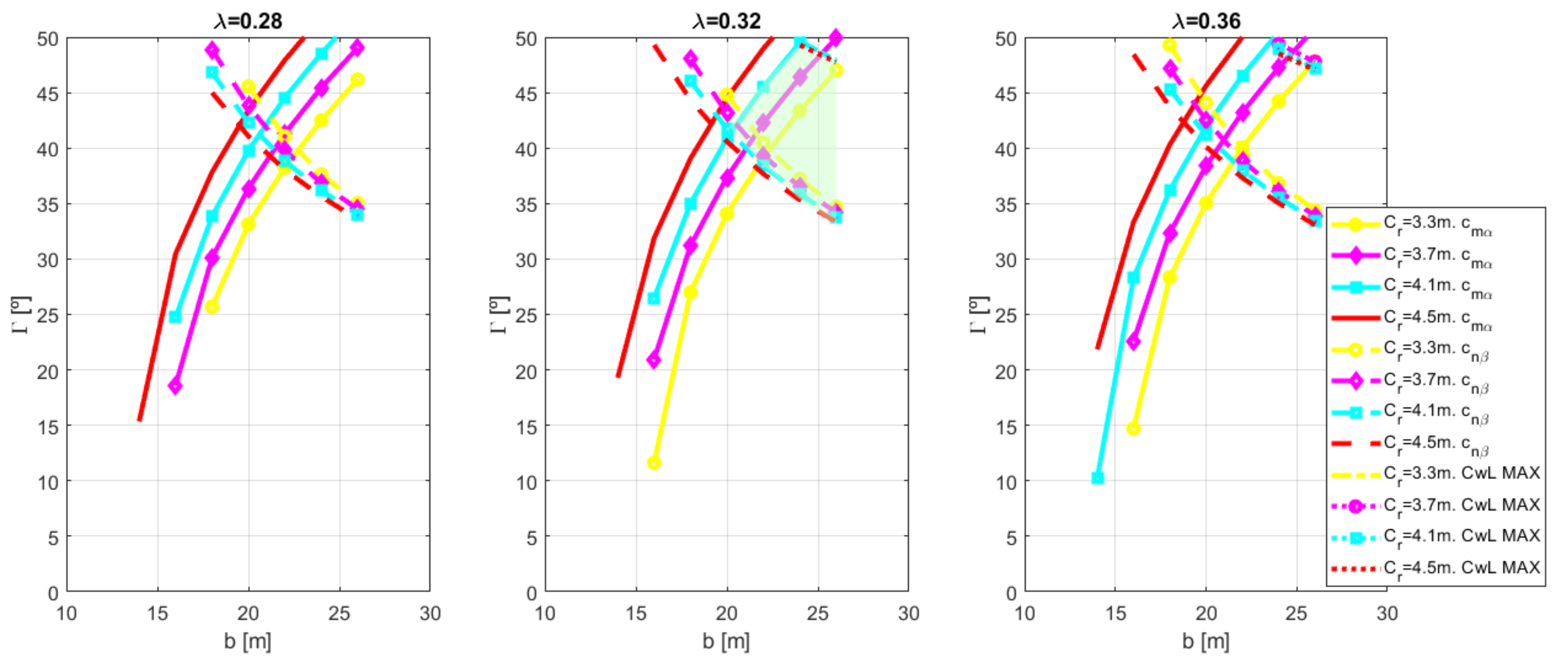
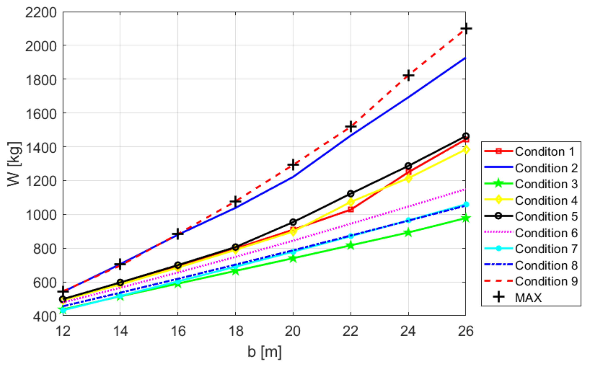
3.2. Unconventional Tail Design

The configuration selected for this case study presented in this paper is V-tail configuration. This selection is based on the fact that it supposes a small change in the external appearance of the aircraft, which would have higher acceptance both by the passengers and the companies. Furthermore, this unconventional configuration is the simplest and most similar to a conventional tail configuration, which makes the validation tasks easier. Despite that, the procedure presented in this paper is thought to be applicable for any other unconventional tail configuration, as long as the limitations of the selected methodologies are not exceeded.

The parameters that define the V-tail geometry are the following: root chord, taper ratio, span, dihedral angle, sweep of $1/4$ chords line, twist angle, relative thickness and airfoil. Some of these parameters can be considered as constant because their influence in performances is reduced, or their values are typical in the state of the art of commercial airplanes. For instance, the airfoil installed on tail surfaces is symmetric in the majority of the aircraft, so it was decided to choose the same airfoil as the horizontal tail surface one of the reference aircraft. For the same reason, the horizontal tail plane of the reference aircraft has zero twist angle along the span, thus it was decided to take the same for the V-tail. Furthermore, the relative thickness was chosen equal to the corresponding to the horizontal tail surface of CSR-01 as well. Finally, the sweep angle of the $1/4$ chords line was fixed at the same value of the horizontal tail surface of the reference aircraft. To sum up, the final parameters under study are root chord, taper ratio, span and dihedral angle. The definitions of these parameters for the V-tail configuration can be found in [24].

Once the geometry is defined, it is necessary to identify the span and the position of the longitudinal and lateral controls. The controls are trailing edge devices that extend from 12.5% to 100% of span. This surface is divided into two controls. The longitudinal one is located in the outboard part of the surface and spans a half of the semispan. On the other hand, the lateral control spans from 12.5% to 50% of the semispan of the V-tail. This design decision is based on the fact that the asymmetric control is considered for controlling the yaw movement of the aircraft, but not the roll. It is true that a coupling between the two movements exists, but it is lower in the case of considering the inner surface as the lateral control instead of the outer one [30].

The feasible design space where the minimum weight must be found is represented in Figure 4. A fully explanation of how this design space is determined is included in [24]. From the four constraints that define this space, there are three active boundaries: static longitudinal stability at cruising conditions, static lateral stability at cruising conditions and maximum negative deflection of lateral control for crosswind landing condition. The design space establishes a combination of the design parameters (taper ratio, root chord, span and dihedral angle) where all conditions are accomplished.

The next step is to evaluate the objective function inside of the feasible design space in order to find the minimum value of the function and the corresponding combination of the design parameters. In the case of V-tail, both symmetric and asymmetric maneuvers introduce loads on the same surface, because both control channels, lateral and longitudinal, are generated in this tail. The maneuvers contemplated to determine the loads for sizing the structure are described in Section 3.1. The numeration established there allows identifying for which maneuver the results are being represented. Additionally, because in the V-tail configuration the lateral and longitudinal maneuvers are coupled, in order to solve any lateral maneuver, it is necessary to balance the aircraft longitudinally beforehand. This fact indicates that lateral maneuvers introduce loads to the structure via two ways: the lateral maneuver itself and the longitudinal balancing. This balancing is performed through two sources: the tail incidence angle and the longitudinal control deflection. It is considered that this tail configuration has fixed incidence angle, and it is determined by balancing the aircraft at cruising conditions. This is to fly at $V_A$ speed at 22,000 ft of altitude, in order not to exceed the boundaries of the aerodynamic model, as happened with the reference aircraft CSR-01.

Among the maneuvers considered in that list, Maneuver 1 requires special mention. A stationary turn is performed such as the lateral control keeps the aircraft flying without sideslip angle. This fact introduces additional loads to the tail surface, which in the reference aircraft does not because it is generated in the vertical tail. In order to be conservative and cover all conditions where both controls are deflected, an additional maneuver is considered for sizing the structure. This is maximum control deflection of both controls at limit and positive load factor at $V_A$ speed. This condition is identified as Condition 9. Finally, it must be highlighted that the load factor associated to the lateral gust depends on the tail geometry because it depends on the lateral force derivative. In consequence, the load factor in lateral gust condition changes according to the combination of the design parameters. For the rest of the maneuvers, the way to model them was carried out as explained for the reference aircraft CSR-01.

Now it is the moment to perform a variation of the design variables in order to determine the bending moment, the shear force and the torsion moment introduced into the structure for each combination of those parameters. Once the loads have been performed for a wide interval of the design variables, the next step is to size the structure in order to estimate the weight of the tail. The procedure is the same as that followed for the reference aircraft. This weight corresponds to the one that is the maximum among the load conditions studied for each combination of the design parameters. Figure 5 represents the weight variation for all load conditions depending on the tail span, for fixed values of the rest of design parameters. Furthermore, the envelope of the maximum weight values for each parameter combination is indicated in it. The shown tendency for the variations of span is qualitatively the same as the tendency of variations in the rest of the design parameters: the weight decreases for lower values of the design variables. In addition, the critical conditions are one and two, depending on the combination of the parameters. In consequence, the optimal of the objective function is reached where the design variables present the lower feasible values. Of course, this optimal must accomplish with the constraints. Furthermore, because of the objective function is monotonous along all the interval of the design parameters, the optimal is reached over the boundary of a constraint [51,52].

Analyzing the monotony along the constraint functions, it is possible to conclude that the active ones are those corresponding to longitudinal static stability and lateral static stability. Keeping in mind the feasible design space shown in Figure 4, the optimum can be found in the geometric place defined by the intersection of these two constraints, because this is precisely where the design parameters reach their lower values. This intersection reduces the degree of freedom of the problem, since a new relation between the design variables is imposed. The resultant combination of the parameters is shown in Figure 6. Therefore, a new feasible design space is defined where the optimal point needs to be found.

In this case, the rule of reaching the lower values of the design parameters does not work anymore, because reducing the root chord will result in an increase of the span. Thus, it is necessary to analyze the behavior of the objective function along this feasible design space. This analysis indicates that the effect of increasing the span is harder than the effect of reducing the root chord. In consequence, the minimum weight is reached when the maximum root chord and taper ratio is obtained. The resultant weight estimation determines that the V-tail weights around 1300 kg.

This result is not relevant if it is analyzed in an isolated way. The important point is how this result affects to the fuel consumption in the route studied for the CSR-01. The designed V-tail configuration presents a reduction of the wetted area, which supposes a reduction on the aerodynamic drag. Equation (1), applied previously for the tail surfaces of the reference aircraft, is used for estimating the zero-lift drag of the V-tail. The only clarification that must be indicated is that the tail area was determined by extending the surface to reach the symmetry plane, in order to consider the interference with the fuselage contribution. In consequence, for reducing the aerodynamic drag, it is necessary to reduce the area of the V-tail. The resulting parasite drag coefficient of varying the design parameters along the new feasible design space is shown in Figure 7. In this case, it is possible to see that the effect of reducing the root chord is harder than the effect of increasing the tail span.

Thus, the effect of minimizing the weight has the opposite effect in the tail drag. In consequence, it is necessary to determine which effect is harder from the standpoint of the fuel consumption in the chosen route. The procedure followed is the same as that explained for the reference aircraft. In this case, it is necessary to consider the changes in weight and drag. For each combination of the design parameters, the new operative empty weight is determined, just removing the weight of the original tail surfaces and adding the corresponding to the unconventional tail. From the standpoint of the polar drag, the procedure consists of substituting the drag of the original tail by the new one. Again, the equation to calculate the fuel consumption is iterative because the Breguet range parameter depends on the takeoff weight of the aircraft, which is the unknown of the problem. Once the problem converged, the results reached are represented in Figure 8. It shows the variation in percentage of the estimated fuel consumption with respect to the one reached for the reference aircraft. It is possible to see that the line for $\lambda =0.36$ crosses the line for $\lambda =0.32$. The combination of forces and moments to which the structure is subjected to in the case of that last point of the line for $\lambda =0.32$ ends in a heavier torsion box than the one to which the weight estimation process converges in the case of the corresponding parameters of the last point of the line for $\lambda =0.36$. These differences found in the torsion box estimation imply that the final weights and, as a consequence, the trip fuel of these both cases are as shown in Figure 8. Finally, Figure 9 represents the variations of the most relevant greenhouse gases emitted by the aircraft in the design route, following the same procedure as the one used for the reference aircraft CSR-01. In the case of NO_x emissions, just those calculated with BFFM2 are represented because they are the most conservative. As the exhaust gas emissions are somehow proportional to the trip fuel consumption, the behaviors of the lines are qualitatively similar to the behavior of the trip fuel consumption, even the crossing of the lines.

4. Discussion

These results point out that the effect of reducing the tail area and, in consequence, the friction drag of the tail is more important for reducing the fuel consumption than the effect of reducing the weight. The optimal reached supposes an increased tail weight of a 30% with respect to the reference aircraft, but the fuel consumption in the design route is reduced by 0.7% with respect the consumption of CSR-01 for the same route. It is necessary to highlight that the Breguet range parameter determined after the convergence procedure for the optimal solution is 25,993.49 km, which is an improvement of that parameter by 1.48%. The fuel reductions determined in this study are aligned with those found in other studies that analyzed the advantages and drawbacks of using V-tail configuration in commercial transport aviation [15]. This study concludes that this tail configuration supposes an increase of weight with respect to the conventional configuration, but the fuel consumption savings are practically neutral. Furthermore, the study reveals that V-tails will suppose a reduction of tail area of around 20%. In this study, the reached optimal design supposes a reduction of the tail area with respect to the reference aircraft of 21%. Thus, the procedure presented in this paper for sizing unconventional tail configuration is validated through the application to the V-tail case study.

Focusing on the environmental impact, the emissions which are considered to be proportional to fuel consumption present the same reductions as it, obviously. As an example, one of them, CO₂, is depicted in Figure 9. On the other hand, NO_x emissions are reduced to a greater extent than savings in trip fuel. This is an important conclusion because it could be a stronger reason for considering this unconventional configuration for future aviation. However, HC and CO emissions are not so reduced. In fact, CO emissions are increased with respect to reference aircraft ones. This is justified when analyzing the ICAO databank, since the selected engine emits more CO for lower fuel flows. As this unconventional configuration needs lower thrust levels to develop cruise flight, lower fuel flow is demanded. In consequence, CO emissions are increased.

In order to carry out the sizing of unconventional tail configurations considering design requirements based on the certification regulations for commercial transport aircraft, several tools are needed for estimating aerodynamics performances and weights. These tools were developed in previous studies, and this paper presents the interaction of those tools and their application of a case study of sizing a V-tail configuration. Their interaction was measured from the standpoint of the impact on the fuel consumption for a certain route of a reference aircraft. Even though tools were validated, they have some limitations that need to be considered. Thus, the decision to perform a comparative study of the results with respect to a reference aircraft tries to reduce the impact of those limitations. The comparative strategy assumes that the inaccuracies reached by the results for the reference aircraft are analogous to the ones reached by the results of the unconventional tail, so the comparative conclusions are more relevant than trying to extract absolute results.

From the standpoint of the selected load cases, the maneuvers cover almost all relevant conditions included in the certification regulations that are compatible with the limitations of the aerodynamic methodology. The aerodynamic tool does not allow considering transonic conditions or situations where the tail is near to stall. Despite that, the load cases considered in this study resulted in an accurate estimation of the stabilizers’ weight for the reference aircraft during the calibration process. Nevertheless, it would be desirable to check this result in future stages of this study. The main drawback is the difficulty to find an aerodynamic tool that allows the user to analyze transonic conditions with the lower computational time required in these early conceptual design stages. Therefore, the study presented in this paper could be considered as a first approximation to the problem in order to reduce the cases that need to be performed with a more complex and more accurate aerodynamic tool.

Despite of the limitations associated to the chosen tools, the presented methodology has been validated for the case study of V-tail configuration. The reductions in terms of tail area and fuel consumption are in line with those predicted by other previous viability studies. However, it is not possible to conclude that this tail configuration will suppose an actual fuel consumption reduction. Keeping in mind that the methodologies used in conceptual design stages have an accuracy of around 5–10%, the resultant savings in terms of fuel consumption are not relevant. The main conclusion that can be extracted from this conceptual design study is that V-tail configuration should be considered for deeper stages of aircraft design process. After a preliminary and more detailed design study, it will be possible to conclude if this configuration is as promising as it seems in this work.

Finally, the extension of this methodology to other configurations is immediate once that configuration is defined in terms of geometrical parameters. However, performing a previous analysis is recommended in order to determine if any limitations of one of the tools is reached. In that case, the corresponding corrections to the methodologies should be implemented.

5. Conclusions

This paper presents a conceptual design tool for sizing unconventional tail configurations for commercial transport aircraft which was calibrated and tested. Furthermore, the selected and modeled load cases for sizing aircraft tails cover almost all relevant conditions included in the certification regulations for commercial transport airplanes, keeping in mind the limitations of the chosen aerodynamic methodology. Despite the limitations of the study, the methodology estimates with enough accuracy the weight of conventional tail surfaces. The case study selected consists of sizing a V-tail configuration and analyzing the impact on the fuel consumption and the greenhouse emissions for a selected route based on a reference aircraft. The results reached for V-tail configurations in terms of fuel savings coincide with those reached in other previous analysis, so the tool is validated. Moreover, the methodology can easily be extended to some other unconventional tail configuration. From the standpoint of the V-tail configuration itself, the resultant fuel savings are not relevant according to the required accuracy for models used in conceptual design, but V-tail configuration is an option that can be considered for preliminary and detailed design study in order to confirm, or not, the fuel savings and reductions in pollutants.

References

1. ACARE (The Advisory Council for Aeronautics Research in Europe). Aeronautics and Air Transport beyond Vision 2020 (Towards 2050); Technical Report; European Commission: Brussels, Belgium, 2010. [Google Scholar]
2. European Aviation Safety Agency. European Aviation Environmental Report; Technical Report; European Aviation Safety Agency: Cologne, Germany, 2019. [Google Scholar]
3. Darecki, M.; Edelstenne, C.; Enders, T.; Fernandez, E.; Hartman, P.; Herteman, J.P.; Kerkloh, M.; King, I.; Ky, P.; Mathieu, M.; et al. Flightpath 2050 Europe’s Vision for Aviation. Report of the High Level Group on Aviation Research Policy; European Commission: Brussels, Belgium, 2011. [Google Scholar] [CrossRef]
4. European Parliament, C.o.t.E.U. Directive 2008/101/EC of the European Parliament and of the Council of 19 November 2008 amending Directive 2003/87/EC so as to include aviation activities in the scheme for greenhouse gas emission allowance trading within the Community. Off. J. Eur. Union 2009, 52, 3–21, ISSN 1725-2555. [Google Scholar]
5. Lee, D.; Pitari, G.; Grewe, V.; Gierens, K.; Penner, J.; Petzold, A.; Prather, M.; Schumann, U.; Bais, A.; Berntsen, T. Transport impacts on atmosphere and climate: Aviation. Atmos. Environ. 2010, 44, 4678–4734. [Google Scholar] [CrossRef] [PubMed] [Green Version]
6. Macintosh, A.; Wallace, L. International aviation emissions to 2025: Can emissions be stabilised without restricting demand? Energy Policy 2009, 37, 264–273. [Google Scholar] [CrossRef] [PubMed]
7. Wasiuk, D.K.; Khan, M.A.H.; Shallcross, D.E.; Lowenberg, M.H. A commercial aircraft fuel burn and emissions inventory for 2005–2011. Atmosphere 2016, 7, 78. [Google Scholar] [CrossRef] [Green Version]
8. BOEING. Commercial Market Outlook 2020–2039; BOEING: Arlington, VA, USA, 2020. [Google Scholar]
9. AIRBUS. Global Market Forecast. Cities, Airports and Aircraft 2019–2038; AIRBUS: CEDEX Blagnac, France, 2019. [Google Scholar]
10. FAA. FAA Aerospace Forecasts Fiscal Years 2020–2040; Technical Report; Forecasts and Performance Analysis Division (APO-100), Federal Aviation Administration: Washington, DC, USA, 2020.
11. Anderson, J. The Airplane: A History of Its Technology; AIAA: Reston, VI, USA, 2002. [Google Scholar]
12. Martinez-Val, R.; Perez, E. Aeronautics and astronautics: Recent progress and future trends. Proc. Inst. Mech. Eng. Part C J. Mech. Eng. Sci. 2009, 223, 2767–2820. [Google Scholar] [CrossRef]
13. Tasca, A.L.; Cipolla, V.; Salem, K.A. Innovative Box-Wing Aircraft: Emissions and Climate Change. Sustainability 2021, 13, 3282. [Google Scholar] [CrossRef]
14. Kroo, I. Nonplanar Wing Concepts for Increased Aircraft Efficiency. In Proceedings of the VKI lecture series of Innovative Configurations and Advanced Concepts for Future Civil Aircraft, Sint-Genesius-Rode, Belgium, 6–10 June 2005; pp. 1–29. [Google Scholar]
15. Frota, J.; Nicholls, K.; Whurr, J.; Müller, M.; Gall, P.E.; Loerke, J.; Macgregor, K.; Schmollgruber, P.; Russell, J.; Hepperle, M.; et al. Final Activity Report. New Aircraft Concept Research (NACRE); Technical Report; SIXTH FRAMEWORK PROGRAMME PRIORITY 4. Aeronautics and Space. FP6-2003-AERO-1; NACRE Consortium: Blagnac, France, 2010. [Google Scholar]
16. Torenbeek, E. Advanced Aircraft Design; John Wiley & Sons, Ltd.: Chichester, UK, 2013. [Google Scholar]
17. Garcia-Benitez, J.; Cuerno-Rejado, C.; Gomez-Blanco, R. Conceptual design of a nonplanar wing airliner. Aircraft Eng. Aerospace Technol. 2016, 88, 561–571. [Google Scholar] [CrossRef]
18. Zhang, C.; Zhou, Z.; Zhu, X.; Meng, P. Nonlinear static aeroelastic and trim analysis of Highly Flexible Joined-Wing aircraft. AIAA J. 2018, 56, 4988–4999. [Google Scholar] [CrossRef]
19. Belardo, M.; Marano, A.D.; Beretta, J.; Diodati, G.; Graziano, M.; Capasso, M.; Ariola, P.; Orlando, S.; Di Caprio, F.; Paletta, N.; et al. Wing Structure of the Next-Generation Civil Tiltrotor: From Concept to Preliminary Design. Aerospace 2021, 8, 102. [Google Scholar] [CrossRef]
20. SAE. Procedure for the Calculation of Aircraft Emissions; Technical Report AIR5715; SAE International: Warrendale, PA, USA, 2009. [Google Scholar]
21. EASA. Introduction to the ICAO Engine Emissions Databank; Technical Report; EASA: Cologne, Germany, 2021. [Google Scholar]
22. Eyers, C.; Norman, P.; Middel, J.; Plohr, M.; Michot, S.; Atkinson, K.; Christou, R. AERO2k Global Aviation Emissions Inventories for 2002 and 2025; Technical Report; QinetiQ Ltd.: Farnborough, UK, 2004. [Google Scholar]
23. Anderson, J.D. Aircraft Performance and Design; WCB McGraw-Hill: Boston, MA, USA, 1999. [Google Scholar]
24. Sanchez-Carmona, A.; Cuerno-Rejado, C. Vee-tail conceptual design criteria for commercial transport aeroplanes. Chin. J. Aeronaut. 2019, 32, 595–610. [Google Scholar] [CrossRef]
25. Torenbeek, E. Synthesis of Subsonic Airplane Design; Delft University Press: Delft, The Netherlands; Kluwer Academic Publishers: Dordrecht, The Netherlands, 1982. [Google Scholar]
26. Roskam, J. Airplane Deisgn. Part V: Component Weight Estimation; DAR Corporation: Ottawa, KS, USA, 1999. [Google Scholar]
27. Raymer, D.P. Aircraft Design: A Conceptual Approach, 1st ed.; American Institute of Aeronautics and Astronautics, Inc.: Washington, DC, USA, 1989. [Google Scholar]
28. Sadraey, M.H. Aircraft Design. A Systems Engineering Approach, 1st ed.; John Wiley & Sons, Ltd.: Chichester, UK, 2013. [Google Scholar]
29. Lucas, S.D.; Velazquez, A.; Vega, J.M. An Optimization Method for an Aircraft Rear-end Conceptual Design Based on Surrogate Models. In Proceedings of the World Congress of Engineering, London, UK, 6–8 July 2011; Volume 3, pp. 2610–2615. [Google Scholar]
30. García-Hernández, L.; Cuerno-Rejado, C.; Pérez-Cortés, M. Dynamics and Failure Models for a V-Tail Remotely Piloted Aircraft System. J. Guid. Control Dyn. 2017, 41, 506–514. [Google Scholar] [CrossRef]
31. Musa, N.A.; Mansor, S.; Ali, A.; Omar, W.Z.W. Importance of transient aerodynamic derivatives for V-tail aircraft flight dynamic design. In Proceedings of the 30th Congress of the International Council of the Aeronautical Sciences, ICAS 2016, Daejeon, Korea, 25–30 September 2016. [Google Scholar]
32. Zhang, G.Q.; Yu, S.C.M.; Chien, A.; Xu, Y. Investigation of the Tail Dihedral Effects on the Aerodynamic Characteristics for the Low Speed Aircraft. Adv. Mech. Eng. 2013, 2013, 1–12. [Google Scholar] [CrossRef] [Green Version]
33. Risse, K.; Schäfer, K.; Schültke, F.; Stumpf, E. Central Reference Aircraft data System (CeRAS) for research community. CEAS Aeronaut. J. 2016, 7, 121–133. [Google Scholar] [CrossRef]
34. Nicolai, L.M.; Carichner, G.E. Fundamentals of Aircraft and Airship Design. Volume I: Aircraft Design, AIAA educa ed.; American Institute of Aeronautics and Astronautics, Inc.: Blacksburg, VI, USA, 2010. [Google Scholar]
35. Sanchez-Carmona, A.; Cuerno-Rejado, C.; Garcia-Hernandez, L. Unconventional Tail Configurations for Transport Aircraft. In Progress in Flight Physics Volume 9; Knight, D.D., Bondar, Y., Lipatov, I.I., Reijasse, P., Eds.; Torus Press: Moscow, Russia; EDP Sciences: Les Ulis, France, 2017; Chapter 1; pp. 127–148. [Google Scholar]
36. Martinez-Val, R.; Roa, J.; Perez, E.; Cuerno, C. Effects of the mismatch between design capabilities and actual aircraft utilization. J. Aircraft 2011, 48, 1921–1927. [Google Scholar] [CrossRef]
37. Martinez-Val, R.; Palacin, J.F.; Perez, E. The evolution of jet airliners explained through the range equation. Proc. Inst. Mech. Eng. Part G J. Aerospace Eng. 2008, 222, 915–919. [Google Scholar] [CrossRef]
38. Melin, T. A Vortex Lattice MATLAB Implementation for Linear Aerodynamic Wing Applications. Master’s Thesis, Royal Institute of Technology (KTH), Stockholm, Sweden, 2000. [Google Scholar]
39. Polhamus, E.C. Charts for Predicting the Subsonic Vortex-Lift Characteristics of Arrow, Delta, and Diamond Wings; Technical Report April, NASA TN D-6243; NASA: Washington, DC, USA, 1971.
40. Certification Specifications and Acceptance Means of Compilance for Large Aeroplanes CS-25. arXiv 2019, arXiv:1011.1669v3. [CrossRef]
41. Airworthiness Standard: Transport Category Airplanes. Title 14—Chapter I—Subchapter C—Part 25 Code of Federal Regulations. 2017. Available online: https://www.faa.gov/aircraft/air_cert/airworthiness_certification/std_awcert/std_awcert_regs/regs/ (accessed on 1 June 2021).
42. Lomax, T.L. Structural Loads Analysis for Commercial Transport Aircraft: Theory and Practice; AIAA Education Series: Reston, VI, USA, 1996. [Google Scholar]
43. Pratt, K. A Revised Formula for Caluclation of Gust Loads; Technical Report, NACA TN 2964; NASA: Washington, DC, USA, 1953.
44. Pratt, K.; Walker, W. Revised Gust Load Formula and a Re-Evaluation of V-G Data Taken on Civil Transport Airplanes from 1933 to 1950; Technical Report, NACA Report 1206; NASA: Washington, DC, USA, 1953.
45. Dababneh, O.; Kipouros, T. A review of aircraft wing mass estimation methods. Aerospace Sci. Technol. 2018, 72, 256–266. [Google Scholar] [CrossRef]
46. Farrar, D. The design of compression structures for minimum weight. J. R. Aeronaut. Soc. 1949, 53, 1041–1052. [Google Scholar] [CrossRef]
47. ICAO. ICAO Aircraft Engine Emissions Databank; ICAO: Montreal, QC, Canada, 2021. [Google Scholar]
48. Schaefer, M.; Bartosch, S. Overview on Fuel Flow Correlation Methods for the Calculation of NOx, CO and HC Emissions and Their Implementation into Aircraft Performance Software; Technical Report; DLR: Cologne, Germany, 2013. [Google Scholar]
49. Dubois, D.B.; Paynter, G.C.B. “Fuel Flow Method 2” for Estimating Aircraft Emissions. SAE Trans. 2006, 115, 1–14. [Google Scholar] [CrossRef]
50. Jelinek, F.; Carlier, S.; Smith, J. The Advanced Emission Model (AEM3)—Validation Report—Version 1.5—Appendices A, B and C; Technical Report; Eurocontrol: Bretigny-sur-Orge, France, 2004. [Google Scholar]
51. Papalambros, P. Monotonicity Analysis in Engineering Design Optimization. Ph.D. Thesis, Stanford University, Stanford, CA, USA, 1979. [Google Scholar]
52. Papalambros, P.Y.; Wilde, D.J. Principles of Optimal Design: Modeling and Computation, 3rd ed.; Cambridge University Press: Cambridge, UK, 2017; p. 484. [Google Scholar]
Figure 1. Airplane drag polar of CSR-01 in clean configuration for different Mach numbers (left); and in take-off, climb, approach and final approach with landing gear extended conditions (right).
Aerospace 08 00175 g001
Figure 2. Torsion box drawing, where height is h t , length is b t , spar web thickness is t L and pitch between stringers is b.
Aerospace 08 00175 g002
Figure 3. Compression load per unit length and shear flux distributions for symmetric loads in horizontal tail surface (left) and for asymmetric loads in vertical tail surface (right).
Aerospace 08 00175 g003
Figure 4. Feasible design space defined by the constraints imposed by static derivatives at cruising conditions, both longitudinal ( c m α ) and lateral ( c n β ), and by the maximum deflection of the lateral control for crosswind landing conditions, establishing a maximum value for the dihedral angle (CwL MAX).
Aerospace 08 00175 g004
Figure 5. Weight estimation of V-tail for the nine conditions studied, for variation in span and for the parameters Γ = 30°, c r = 3.7 m and λ = 0.32.
Aerospace 08 00175 g005
Figure 6. Design variables combination resulting of intersecting the constraints associated with the static stability conditions, both longitudinal and lateral.
Aerospace 08 00175 g006
Figure 7. Friction drag coefficient as a function of the taper ratio and root chord along the new feasible design space determined intersecting the active constraints.
Aerospace 08 00175 g007
Figure 8. Fuel consumption variation with respect to the reference aircraft for the design route as a function of the taper ratio and root chord along the new feasible design space determined by intersecting the active constraints.
Aerospace 08 00175 g008
Figure 9. Emissions variation with respect to the reference aircraft for the design route as a function of the taper ratio and root chord along the new feasible design space determined by intersecting the active constraints.
Aerospace 08 00175 g009