Article

Multi-Aircraft Trajectory Collaborative Prediction Based on Social Long Short-Term Memory Network

College of Civil Aviation, Nanjing University of Aeronautics and Astronautics, No. 29 General Avenue, Nanjing 211106, China
*
Author to whom correspondence should be addressed.
Aerospace 2021, 8(4), 115; https://doi.org/10.3390/aerospace8040115
Submission received: 18 March 2021 / Revised: 10 April 2021 / Accepted: 12 April 2021 / Published: 19 April 2021

Abstract

:
Aircraft trajectory prediction is the basis of approach and departure sequencing, conflict detection and resolution and other air traffic management technologies. Accurate trajectory prediction can help increase the airspace capacity and ensure the safe and orderly operation of aircraft. Current research focuses on single aircraft trajectory prediction without considering the interaction between aircraft. Therefore, this paper proposes a model based on the Social Long Short-Term Memory (S-LSTM) network to realize the multi-aircraft trajectory collaborative prediction. This model establishes an LSTM network for each aircraft and a pooling layer to integrate the hidden states of the associated aircraft, which can effectively capture the interaction between them. This paper takes the aircraft trajectories in the Northern California terminal area as the experimental data. The results show that, compared with the mainstream trajectory prediction models, the S-LSTM model in this paper has smaller prediction errors, which proves the superiority of the model’s performance. Additionally, another comparative experiment is conducted on airspace scenes with aircraft interactions, and it is found that S-LSTM has a better prediction effect than LSTM, which proves the effectiveness of the former considering aircraft interaction.

1. Introduction

With the increasing flight density in the airspace, how to make full use of the limited airspace resources has become increasingly urgent. Therefore, the industry has increased the research and development of intelligent air traffic management (ATM) tools. The purpose is to provide controllers with intelligent auxiliary decision-making tools to help detect and resolve conflicts, order approach and departure, monitor abnormal aircraft behavior, and manage traffic. However, these automated decision support systems rely on high-precision and reliable aircraft trajectory prediction. As the current ATM mode based on airspace sectors has certain limitations in predictability, efficiency, and safety, it cannot meet future high-density traffic requirements. With the development of NextGen [1] in the United States and Single European Sky ATM Research (SESAR) [2] in Europe, a new trajectory-based operation (TBO) ATM mode has been promoted. The mode shares the dynamic information of the trajectory among air traffic control, airlines, and aircraft based on the accurate 4D aircraft trajectory prediction to realize collaborative decision-making between flight and control. This will help reduce the workload of controllers, increase the airspace capacity, improve airspace resource utilization, and ultimately achieve effective management in high-density, large-flow, and small-interval airspace. In general, trajectory prediction plays a vital role in the ATM system, whether in the current sector-based operation or the future TBO.
Aircraft are susceptible to flight intentions, control behaviors, unstable weather conditions, and other uncertain factors during flight. Therefore, they are discussed to improve the accuracy and reliability of aircraft trajectory prediction. Usually, the uncertain factors will change the flight state or planned trajectory of the affected aircraft. For example, when convective weather or flow control occurs in a certain local area, it will affect the aircraft that originally planned to fly over the area, forcing them to deviate from the planned trajectory. In other words, the uncertain factors are indirectly reflected in the changes in the aircraft’s flight state and planned flight trajectory. If the relationship between aircraft trajectories can be considered when constructing the trajectory prediction model, the uncertain factors are indirectly considered. Figure 1 shows a schematic diagram of the interaction between multiple aircraft in certain airspace. It can be seen from the figure that the aircraft may be affected by aircraft within a certain range in front of them rather than the rear, whether it is at the same or different altitudes. For example, the aircraft ahead does not follow the prevailing trajectory, which means that some uncertain factors (such as convective weather) have appeared ahead. If this information can be used to predict the current aircraft trajectory, it will help improve prediction accuracy.
The Long Short-Term Memory (LSTM) network can effectively capture the long-term dependencies of sequences and has been successfully applied to various time series prediction tasks in recent years [3,4,5]. In previous research, we proposed a single aircraft trajectory prediction model based on deep LSTM, which did not consider the interaction between aircraft [6]. This paper will consider the interaction between aircraft and establish a multi-aircraft trajectory collaborative prediction model based on Social Long Short-Term Memory (S-LSTM). Since the hidden state in the LSTM network structure represents the spatio-temporal characteristics of aircraft, S-LSTM establishes an LSTM network for each aircraft and establishes a pooling layer to share the hidden state information of the associated network, which can effectively capture the interactive information between the aircraft. Therefore, the model is employed for the research-at-hand. In addition, the method in this paper is a 4D trajectory generation model of multiple aircraft. The input sequence is the historical trajectory of multiple aircraft, and the output is the corresponding predicted value of the future trajectory.

2. Related Work

In recent years, many scholars have performed a great deal of research on aircraft trajectory prediction. Now, there are three mainstream prediction methods for this problem: state estimation models, kinetic models, and machine learning models.

2.1. State Estimation Models

The state estimation models construct the state transition matrix in the state equation through the motion equation. They do not involve the aircraft’s mass, force, and other performance parameters but study the relationship between the position at each time point in the future and the historical position, velocity, acceleration, angle, etc. They are also divided into single-model estimation and multi-model estimation according to different assumptions about whether the aircraft has a single mode or multiple flight modes in the prediction process. In single-model estimation, the Kalman filter (KF) algorithm [7,8], particle filter algorithm [9], hidden Markov model (HMM) [10,11,12,13], and their various improved algorithms [14] have been applied in trajectory prediction. When using the KF algorithm for short-term trajectory prediction, Chatterji [7] used the current ground speed, trajectory angle estimation and kinematic equations to propagate the current position estimate forward to obtain the future estimate. Although single-model estimation models have been widely used and achieve certain results, they cannot estimate the hybrid system well with different modes. The aircraft trajectory prediction problem can be regarded as a Stochastic Linear Hybrid System (SLHS) estimation problem, which needs to be solved by the multi-model estimation. As an important method to solve the SLHS estimation problem, the computational cost of the multi-model algorithm increases exponentially with time. Therefore, the generalized Pseudo-Bayes algorithm, interacting multiple model (IMM), and other suboptimal algorithms are proposed. In particular, the IMM algorithm has excellent performance and low computational cost and has been successfully applied to trajectory prediction [15]. However, the standard IMM algorithm assumes that the residual is zero mean and calculates the mode transition probability through the likelihood function. This assumption is usually invalid due to the incompleteness of the mode set in the IMM algorithm. Therefore, many researchers have proposed improved multi-model estimation methods [16,17,18,19]. Zhang et al. [17] proposed an improved IMM algorithm, abandoning the assumption that the likelihood function is a zero-mean Gaussian function, and defined a new likelihood function to update the flight mode probability. In addition, the multi-model estimation models the flight mode transition as a Markov process with a constant mode transition probability matrix, independent of continuous state variables [15]. However, the behavior of an aircraft consists of discrete transitions between many flight modes (discrete states) and continuous motion (continuous state) corresponding to specific flight modes. Therefore, many documents try to model the transition probability of aircraft flight mode depending on its continuous state (such as position, speed, etc.) [20,21,22,23]. Seah et al. [20,21] proposed a multi-model KF algorithm based on the continuous state-dependent mode transition matrix to solve the aircraft trajectory prediction.

2.2. Kinetic Models

The kinetic models mainly study the relationship between the force acting on the aircraft and its motion. They are usually expressed as a set of differential equations. Given the current state of the aircraft, meteorological conditions, and aircraft intentions, the continuous points of the future trajectory can be predicted by integrating differential equations in a time interval. Therefore, this method integrates aircraft intention, performance parameters, and meteorological environment data for calculation. The point mass model (PMM) is the most widely used to model aircraft motion in a fast simulation environment [24,25,26]. Fukuda et al. [24] used PMM to model aircraft motion, and the work rate of force acting on aircraft was equal to the increased rate of potential energy and kinetic energy. Since the motion of the aircraft is an SLHS with different flight modes, it is more reasonable to establish motion equations corresponding to different flight modes. Therefore, many scholars use PMM to predict under SLHS [27,28,29]. Unified and comprehensive intent information is necessary for trajectory prediction. At present, related studies have expanded and improved the flight script to provide a formalized aircraft intent description language [30,31,32,33]. Félix et al. [30] designed a computer formal language to express aircraft intentions, which combined standard operating procedures, airline operating preferences, and the actual pilot’s decision-making process. Aircraft performance parameters provide the aircraft performance data required by the kinetic models. These parameters are related to the type of aircraft, the current motion state of the aircraft (position, speed, weight, etc.), the current atmospheric conditions, and aircraft intention. Aiming at the problem that performance parameters are difficult to obtain, there are some related studies [34,35]. Thipphavong et al. [34] proposed a universal real-time adaptive weighting algorithm to improve the accuracy of climb trajectory prediction. It dynamically adjusted the weight of the aircraft in the model through the available radar trajectory and weather data without any additional information from the aviation operation center or the aircraft. Meteorological data provide information related to the environment, such as temperature, wind direction and speed, air pressure, gravity, and magnetic force changes. Presently, the most popular meteorological databases include the European Centre for Medium-Range Weather Forecasts (ECMWF) and the North American Mesoscale Forecast System (NAM). When environmental information cannot be obtained, estimated values are sometimes used instead. Given the problems of diverse meteorological data formats and sources, some documents have researched the application of specific types of data in trajectory prediction problems.

2.3. Machine Learning Models

The machine learning models mainly mine the laws of trajectory change over time from a large amount of data and use them to predict trajectory. On the one hand, they mainly rely on the similarity of trajectories to mine representative trajectory patterns. On the other hand, they are based on the reconstruction of input and output space [26]. Here, they are divided into regression models, neural networks, and other methods.
At present, the commonly used regression methods in trajectory prediction include local weighted linear regression (LWLR), local weighted polynomial regression, etc. Leege et al. [36] took the actual trajectory and meteorological data as the model’s input and used the stepwise regression method to predict the arrival time. Hamed et al. [37] used standard linear regression models, neural networks, and local weighted regression to predict the height of aircraft climb, and then used principal component analysis to reduce the input data’s dimensionality. Tastambekov et al. [38] established a local linear regression model for trajectory prediction based on historical radar trajectory data without using any physical or aviation parameters.
Since neural networks (NNs) can approximate any continuous mapping well, it is a suitable improvement method compared to general linear regression. At present, more and more researchers use NNs to deal with trajectory prediction problems [39,40,41,42,43,44,45,46,47,48,49,50,51,52]. Commonly used methods include Back Propagation (BP) NN, LSTM and Deep Neural Networks (DNNs), etc. NNs usually take aircraft position and related information as input features and output the probability distribution of the 3D position at multiple points, estimated flight time, or trajectory in the future. Fablec et al. [39] used NN to solve vertical trajectory prediction in the two cases of trajectory prediction during aircraft flight and trajectory generation before aircraft takeoff. Shi et al. [40] proposed a trajectory prediction model based on LSTM that considered the correlation between adjacent states of the trajectory sequence. Wu et al. [45] studied a 4D trajectory prediction model based on BP NN. Hang et al. [47] proposed establishing a hybrid model of DNN and LSTM and used DNN single-step prediction to correct LSTM multi-step prediction. Aiming at the weather-related aircraft trajectory prediction, Pang et al. [49] proposed a new conditional generation confrontation network method and used convolutional layers to extract weather features. Pang et al. [48] used Dropout as a Bayesian approximate variational inference to implement a Bayesian neural network, and finally output a predicted trajectory with a confidence interval.
In addition to regression models and neural networks, other machine learning methods have also appeared [53,54,55], such as genetic algorithm (GA), ant colony algorithm, and support vector machine (SVM), etc., as a separate category here. Current trajectory prediction also uses clustering algorithms [56,57,58,59], such as K-means, Density-Based Spatial Clustering of Applications with Noise (DBSCAN), etc., and usually designs appropriate trajectory similarity metrics to improve the clustering effect. Tang et al. [56] proposed an adaptive clustering method that combines the time deviation edit distance similarity measurement index with the K-means algorithm to improve the nominal flight profile accuracy. Combining clustering with machine learning prediction methods can significantly improve the prediction accuracy of large-scale clusterable data sets. Therefore, the combination of machine learning and clustering for trajectory prediction is a valuable and meaningful research topic. Barratt et al. [58] studied a probabilistic trajectory generation model in the terminal airspace. They used K-means to cluster trajectories and then constructed a Gaussian mixture model from the clusters to achieve accurate trajectory inference. Le et al. [59] proposed a sector-based short-term trajectory prediction method, which divided multiple trajectory clusters according to the spatial behavior of the historical trajectory in the sector and used the random forest algorithm to train the corresponding model.
The first two methods usually require explicit modeling of the aircraft’s real-time state, aircraft performance, and procedures, but most model parameters are not always available at all times (such as aircraft take-off quality, pilot operation differences, etc.), which makes them have certain limitations in practical applications. In contrast, machine learning models do not require explicit modeling of aircraft performance, procedures, and airspace. They mainly learn the spatiotemporal characteristics and operating rules of trajectory information from a large amount of historical aircraft trajectory data. They are constructed under weak or even no assumptions. In some cases, machine learning models can show better prediction performance.
The current studies mainly focus on a single aircraft’s trajectory, hardly consider the interaction between multiple trajectories and predict multiple trajectories simultaneously, which is likely to affect the accuracy of machine learning methods. Faced with this situation, it is necessary to research multiple aircraft trajectory prediction problems.
Inspired by [60], Alahi et al. proposed an S-LSTM model to predict pedestrians’ trajectories in crowded spaces, which uses the “social pool” layer to connect each individual’s LSTM network to share their information. In view of the good effect of the model in pedestrian trajectory prediction, this paper tries to apply it to multi-aircraft trajectory prediction. Compared with previous research work on aircraft trajectory prediction, our research has the following innovations: (1) It considers the interaction between adjacent trajectories; (2) It converges multiple aircraft trajectories into a predictive model, and it can generate multiple 4D trajectories simultaneously given past information.

2.4. Method Overview

In the multi-aircraft trajectory prediction problem, the number of aircraft in certain airspace gradually changes with time. The number of aircraft at time t is N ( t ) , the state vector (longitude, latitude, altitude, speed and angle) of the n - th aircraft is X t n , and the position (longitude, latitude and altitude) of the n - th aircraft is Y t n . Since each aircraft enters the airspace at a different time, the length of each aircraft’s trajectory sequence is different. Assuming that the n - th aircraft enters the airspace at time τ , the state sequence and 4D trajectory sequence of the n - th aircraft at W i time t are S τ , t n = { X τ n , , X t 1 n , X t n } and P τ , t n = { Y τ n , , Y t 1 n , Y t n } , respectively. The goal of this paper is to predict the future 4D trajectory based on the historical state information of multiple aircraft, that is, to construct a predictor F that maps the set of historical state sequences { S τ 1 , t 1 , S τ 2 , t 2 , S τ N ( t ) , t N ( t ) } to { P t , t + Δ T 1 , P t , t + Δ T 2 , P t , t + Δ T N ( t ) } :
S τ 1 , t 1 , S τ 2 , t 2 , S τ N ( t ) , t N ( t ) F P t , t + T 1 , P t , t + T 2 , P t , t + T N ( t )
where T represents the forecast duration.
It can be seen from Equation (1) that each aircraft uses not only its historical state information but also related multiple aircraft state information. This paper will build a multi-aircraft trajectory prediction model under the framework of the deep LSTM theory. The main challenges are as follows:
(a)
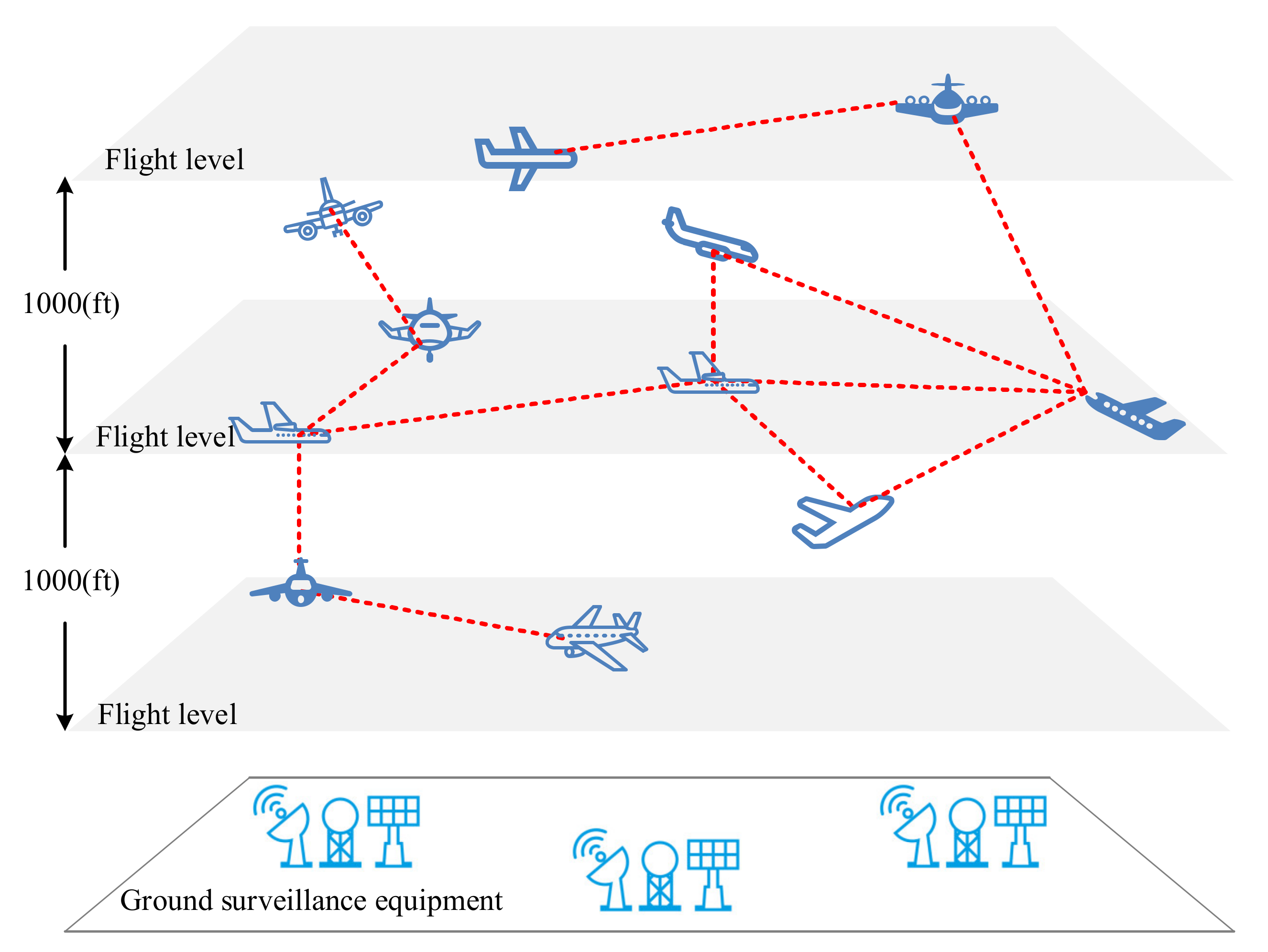
In order to simultaneously predict the 4D trajectory of multiple aircraft at any time, it is necessary to encode the aircraft state sequence dynamically. On the one hand, each aircraft enters and exits the airspace at different time points. How to dynamically update the historical state information input to the model is problematic. On the other hand, inputting the state sequence of multiple aircraft as a whole will cause the input dimension to be too high. How to balance the model’s generalization ability and computational efficiency is another problem.
(b)
How to reasonably consider the interaction between aircraft in the airspace is another significant difficulty in constructing a high-precision trajectory prediction model. Usually, during aircraft flight, the controller will perform conflict resolution based on the aircraft’s flight trend, specified minimum interval, and sector capacity to avoid collisions between aircraft or seek a balance between sector demand and capacity. For example, controllers sometimes designate aircraft to deviate from planned routes to relieve congestion in the airspace sector. This kind of trajectory deviation cannot be predicted by observing an aircraft alone, but other aircraft around which are most likely to affect it need to be considered.
Facing the problem of multi-aircraft trajectory prediction, it is necessary to establish a model to explain the behavior of other aircraft within a certain range and predict the trajectories of all aircraft at the same time. An LSTM network is built for each aircraft to avoid the data dimension being too large during simultaneous prediction. At the same time, a reasonable model integration method must be selected to connect multiple LSTM models to consider the interaction of adjacent aircraft (this connection method will be described in detail later). In the model training stage, the optimal sequence length, the number of neurons in each layer, the size of each batch of training samples, and the number of iterations are determined by adjusting the parameters of the integrated model to determine the optimal prediction model. In the trajectory reasoning stage, the entire flight trajectories of the aircraft can be iteratively predicted by inputting their initial state into the optimized model.

3. Methods

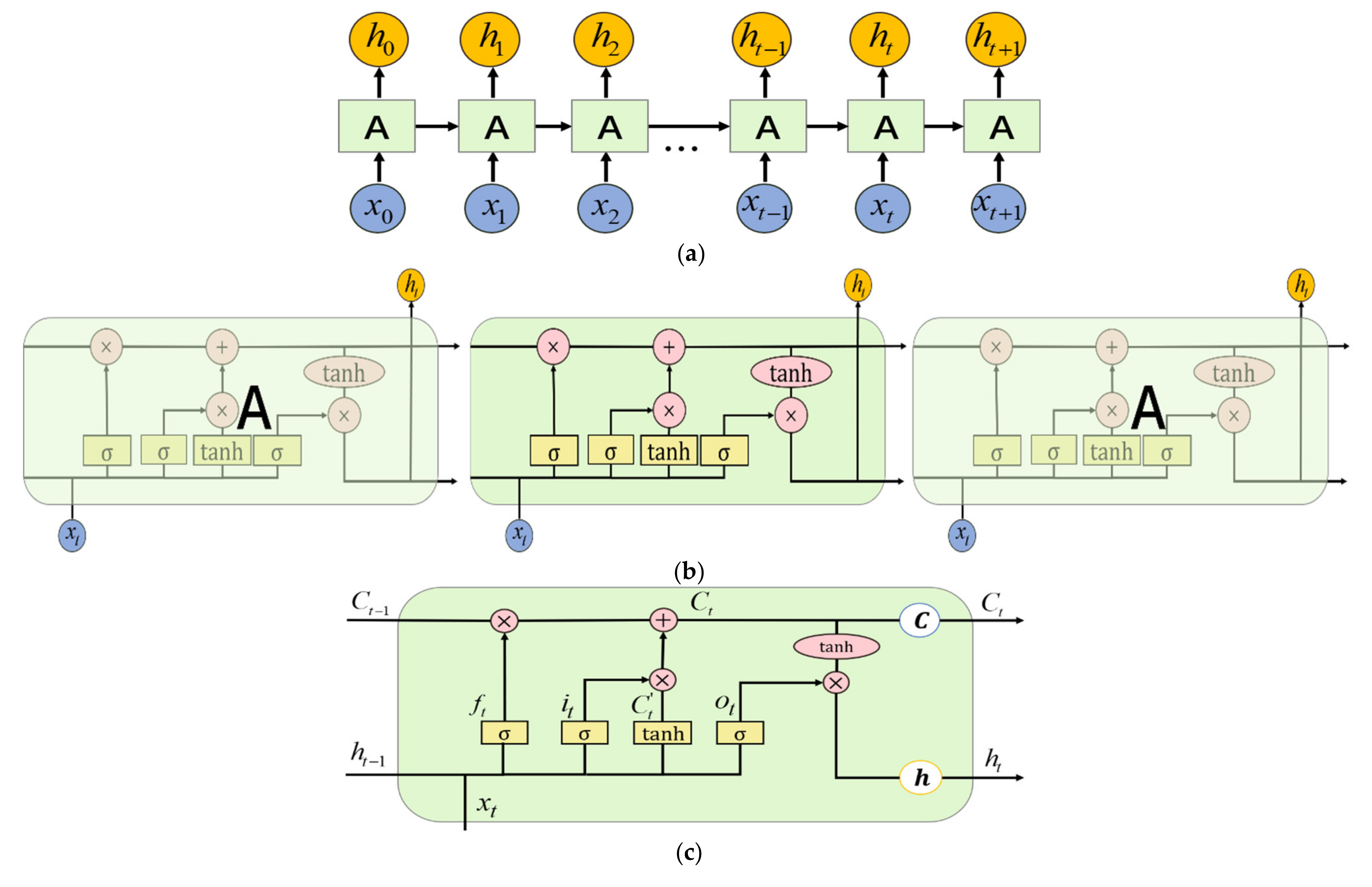
3.1. The Structure of LSTM

LSTM NN is an extension of the recurrent NN (RNN). RNN has good modeling performance for nonlinear time series data. However, it has gradient disappearance and gradient explosion problems, so that it cannot fit the time series with long time steps well. LSTM is specially developed to overcome the limitations of RNN in terms of long-term dependence [61]. A typical LSTM consists of an input layer, one or more hidden layers, and an output layer. Its recurrent structure is similar to RNN, as shown in Figure 2a. The overall network structure of LSTM is shown in Figure 2b. The processing unit A in the hidden layer is different from RNN. This special processing unit includes three gates: forget gate, input gate, and output gate, which are used to control and change the state of the unit and can better deal with long-term dependence issues. Figure 2c specifically shows how the forget gate, input gate, and output gate work. The detailed computation process is shown in Equation (2) [3]:
f t = σ ( W f [ h t 1 , x t ] + b f ) i t = σ ( W i [ h t 1 , x t ] + b i ) C t = tanh ( W C [ h t 1 , x t ] + b C ) C t = f t C t 1 + i t C t o t = σ ( W o [ h t 1 , x t ] + b o ) h t = o t tanh ( C t )
where σ ( ) is the Sigmoid activation function, and tanh ( ) is the hyperbolic tangent activation function. W f , W i , W C , and W o are the weights of the LSTM network layer, and b f , b i , b C , and b o are the bias vectors of the network layer. * in Equation (2) means Hadamard product. In the process of generating the hidden state, the forget gate determines the information that should be deleted from the previous cell state C t 1 . It uses the Sigmoid function as the activation function, and f t is the activation value. The input gate determines what information should be put into the current cell state C t . It uses the Sigmoid function as the activation function, and i t is the activation value. C t is the candidate state calculated using the hyperbolic tangent activation function at the current moment, which combines the cell state at the previous moment, the results of the forget gate and input gate to calculate the new cell state C t .The output gate is used to generate the output hidden state information h t . It uses the Sigmoid function as the activation function, and o t i is the activation value. h t is the hidden state output by the LSTM layer at time t .

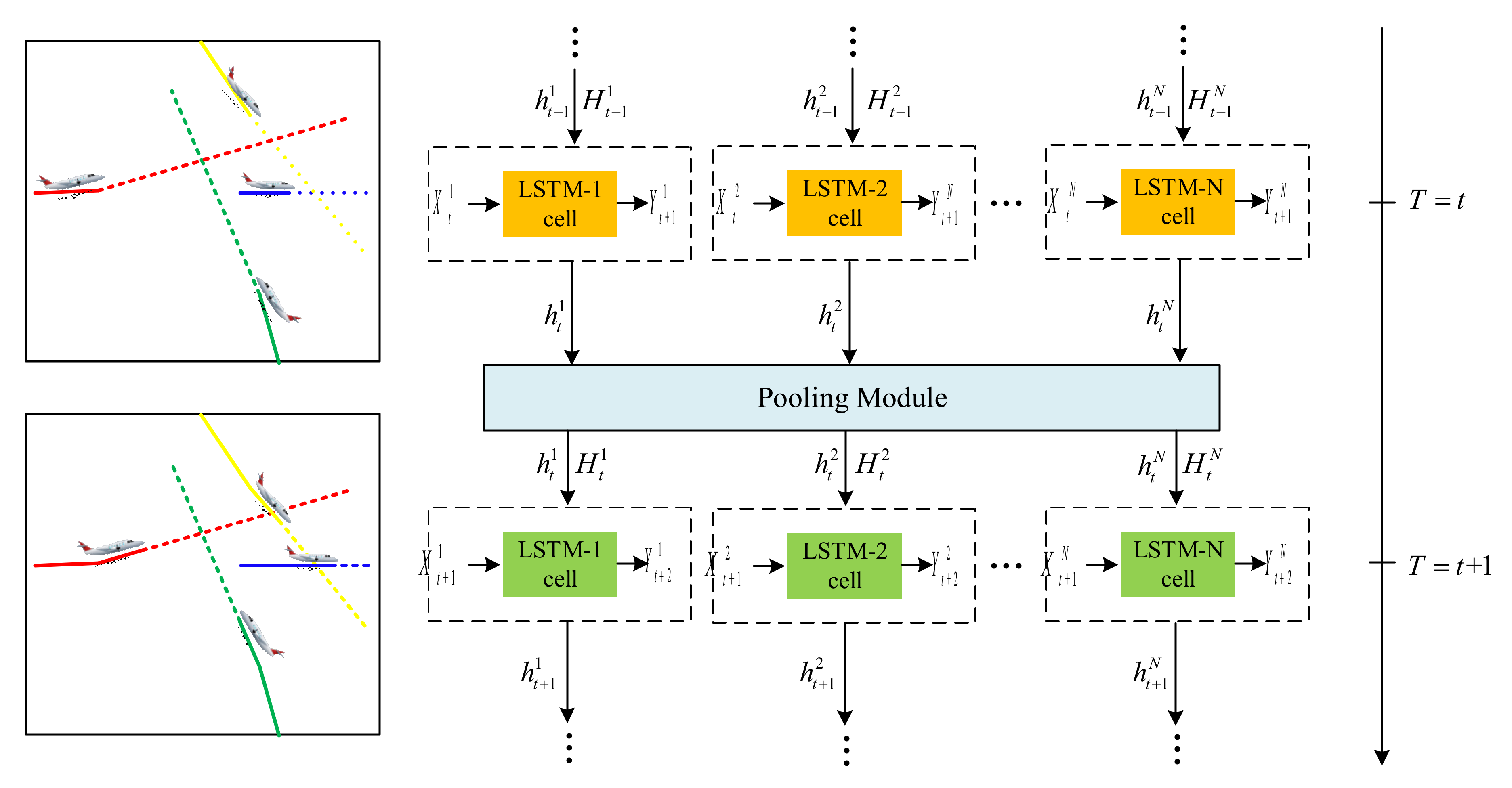
3.2. The Structure of Social LSTM
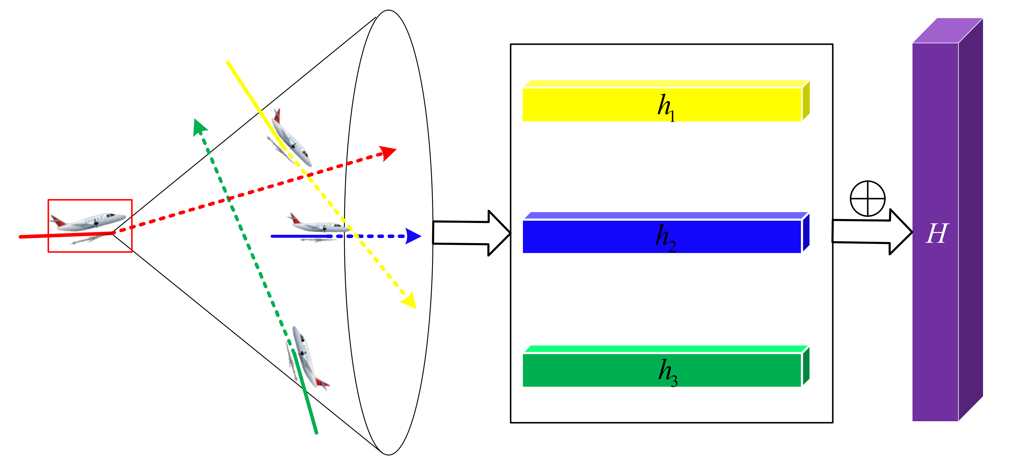
In response to the above two challenges, this paper proposes a pool-based S-LSTM model that can simultaneously predict all aircraft trajectories in the scene. The model structure is shown in Figure 3. Next, the model will be introduced in detail.
S-LSTM has two main improvements compared with LSTM. First of all, a separate LSTM network is established for each aircraft in the scene to synchronize predictions. As shown in Figure 3, the state sequence of each aircraft is input into its own network to avoid the problem of excessively high dimensions of input information. At the same time, the input historical state information can be dynamically updated according to the different times when each aircraft enters and exits the airspace. Secondly, a new pooling strategy is used to connect adjacent LSTMs to filter out the aircraft information that may affect itself and input the filtered information into the corresponding network. Finally, the interaction between adjacent aircraft is captured. This pooling strategy corresponds to the pooling module in Figure 4, and the specific content will be introduced later.

3.3. Pooling Layers

Since the hidden state of each aircraft’s LSTM network generally contains its important spatiotemporal characteristics, it makes sense to share the hidden state between adjacent LSTM networks to consider the interaction of adjacent aircraft. However, each aircraft has a different number of adjacent objects, and especially in a very dense airspace scene, their number is greater, resulting in a larger received hidden state dimension.
Therefore, the model uses a unified representation to combine the hidden state information from all adjacent objects of the aircraft. This problem is dealt with by introducing the pool layer shown in Figure 4: First, it is necessary to filter other aircraft in a certain space in front of the target aircraft because the aircraft trajectory belongs to 3D space coordinates, and then project all aircraft onto the same plane. Finally, a grid-based method is used to keep the received hidden state and integrate the information. At each time step, the LSTM unit will receive the combined hidden state information from other adjacent units. The specific calculation process is as follows.
h t i represents the hidden state generated by the LSTM of the i - th aircraft in the airspace scene at time t , which is a potential representation of the aircraft’s spatiotemporal characteristics. The social hidden state tensor H t i of the i - th aircraft is constructed through the hidden state shared by other adjacent LSTMs to realize the interaction between multiple LSTMs. When given a hidden state dimension D , a neighborhood size δ , and a merge window size N 0 , the model uses the i - th aircraft as the center to determine the other aircraft within its front neighborhood, and uses their hidden state at this time to construct a N 0 × N 0 × D dimensional tensor for the i - th aircraft:
H t i ( m , n , : ) = j Q t i 1 m n [ x t j x t i , y t j y t i , z t j z t i ] h t 1 j
where h t 1 j corresponds to the hidden state of LSTM of the j - th aircraft at time t 1 , and x t i , y t i and z t i represent the spatial position of the i - th aircraft. 1 m n [ x , y , z ] is an indicator variable, where m , n [ 1 , N 0 ] is used to check whether ( x , y , z ) is in cell ( m , n ) of the grid. If the j - th aircraft falls in this cell, the indicator variable takes the value 1, otherwise it is 0. Q t i is the set of aircraft adjacent to the i - th aircraft at time t . H t i ( m , n , : ) represents the combined information in cell ( m , n ) . It can be seen from Equation (3) that this method only retains the hidden state of the aircraft in the specified neighborhood.
The model embeds the pooled social hidden state tensor H t i into the vector a t i , and embeds the 3D coordinates of the i - th aircraft into e t i . Then, a t i and e t i are input to the LSTM network of the i - th aircraft at time t . The process is shown in Equation (4):
a t i = ϕ ( W a [ H t i ] + b a ) e t i = ϕ ( W e [ x t i , y t i , z t i ] + b e ) h t i = L S T M ( h t 1 i , e t i , a t i ; W l , b l )
where ϕ ( ) is the rectified linear unit activation function, W a and W e are the weights of the embedding layer, and b a and b e are the bias vectors of the embedding layer. W l is all the weights of the LSTM network layer, b l is all the bias vectors of the network layer, h t i is the hidden state output by the LSTM layer of the i - th aircraft at time t .

3.4. Trajectory Inference Process

In order to estimate the trajectory, the model first estimates the position at the current moment, and then predicts the position at the next moment based on the estimated value. In the model training stage, the hidden state at time t 1 is used to predict the distribution of the trajectory position x ^ t i , y ^ t i , z ^ t i at the next time t . Assuming that the 3D trajectory of the aircraft obeys the ternary Gaussian distribution, its distribution parameters include: the mean is μ t i = ( μ x , μ y , μ z ) t i , and the covariance matrix is t i = σ x 2 C o v ( x , y ) C o v ( x , z ) C o v ( x , y ) σ y 2 C o v ( y , z ) C o v ( x , z ) C o v ( y , z ) σ z 2 . In order to ensure the positive definiteness of the covariance matrix, the prediction network outputs the lower triangular component L t i of the covariance matrix, which is further constructed by Cholesky decomposition, as shown in Equation (6). These parameters are predicted by a linear layer with a 9 × D dimensional weight matrix W L , as shown in Equation (7). The predicted coordinate ( x ^ t i , y ^ t i , z ^ t i ) at time t is given by Equation (5):
( x ^ t i , y ^ t i , z ^ t i ) N ( μ t i , t i )
t i = L t i L t i T
[ μ t i , L t i ] = W L h t 1 i
L i ( W , b ) = t = 1 T o b s log ( P ( x t i , y t i , z t i | μ t i , t i ) )
here, the negative log-likelihood loss is selected as the loss function of the model to learn the parameters of LSTM, including all weights and biases mentioned earlier. For example, the loss function L i of the i - th trajectory is shown in Equation (8), ( x t i , y t i , z t i ) , respectively, represents the real 3D position coordinates at time t , and P ( ) represents the probability of the real coordinates at time t in the corresponding probability distribution. Since there are multiple aircraft in the airspace at time t , the model is trained by minimizing the sum of the loss functions of all aircraft trajectories in the training data set, that is, backpropagation through multiple LSTMs in the airspace. However, it should be noted that S-LSTM connects multiple LSTM networks to simultaneously predict through the pooling layer. The essence is still that each LSTM is back-propagated separately at the same time, which shows that the back-propagation process of the S-LSTM in this paper is actually similar to an LSTM network. In addition, the LSTM network itself can effectively avoid the gradient explosion problem through a unique gate design function. Therefore, it is believed that S-LSTM is unlikely to have such a problem.
In the trajectory reasoning stage, the trained S-LSTM model is used to predict the future position ( x ^ t i , y ^ t i , z ^ t i ) of the i - th aircraft. From time step T o b s + 1 to T p r e d , the predicted value ( x ^ t i , y ^ t i , z ^ t i ) at the previous moment is used to replace the real value ( x t i , y t i , z t i ) to calculate the social hidden state tensor H t i , which is input into the network together with ( x ^ t i , y ^ t i , z ^ t i ) at the next moment, and finally predict the entire trajectory through continuous iteration.

4. Case Analysis

This section used the flight trajectories over the San Francisco Bay Area in the United States for example analysis. The appropriate S-LSTM model was determined by adjusting the hyperparameters, and the appropriate performance evaluation index was selected. In the experiment, the prediction error of the model in this paper was compared with the current mainstream trajectory prediction model to evaluate the performance of the model. At the same time, statistical analysis was performed on the prediction errors of departure and arrival flights in different time intervals to observe the differences in the performance of our models. In addition, a suitable airspace scene was selected to analyze and discuss the prediction results visually to verify that S-LSTM considers the interaction between aircraft.

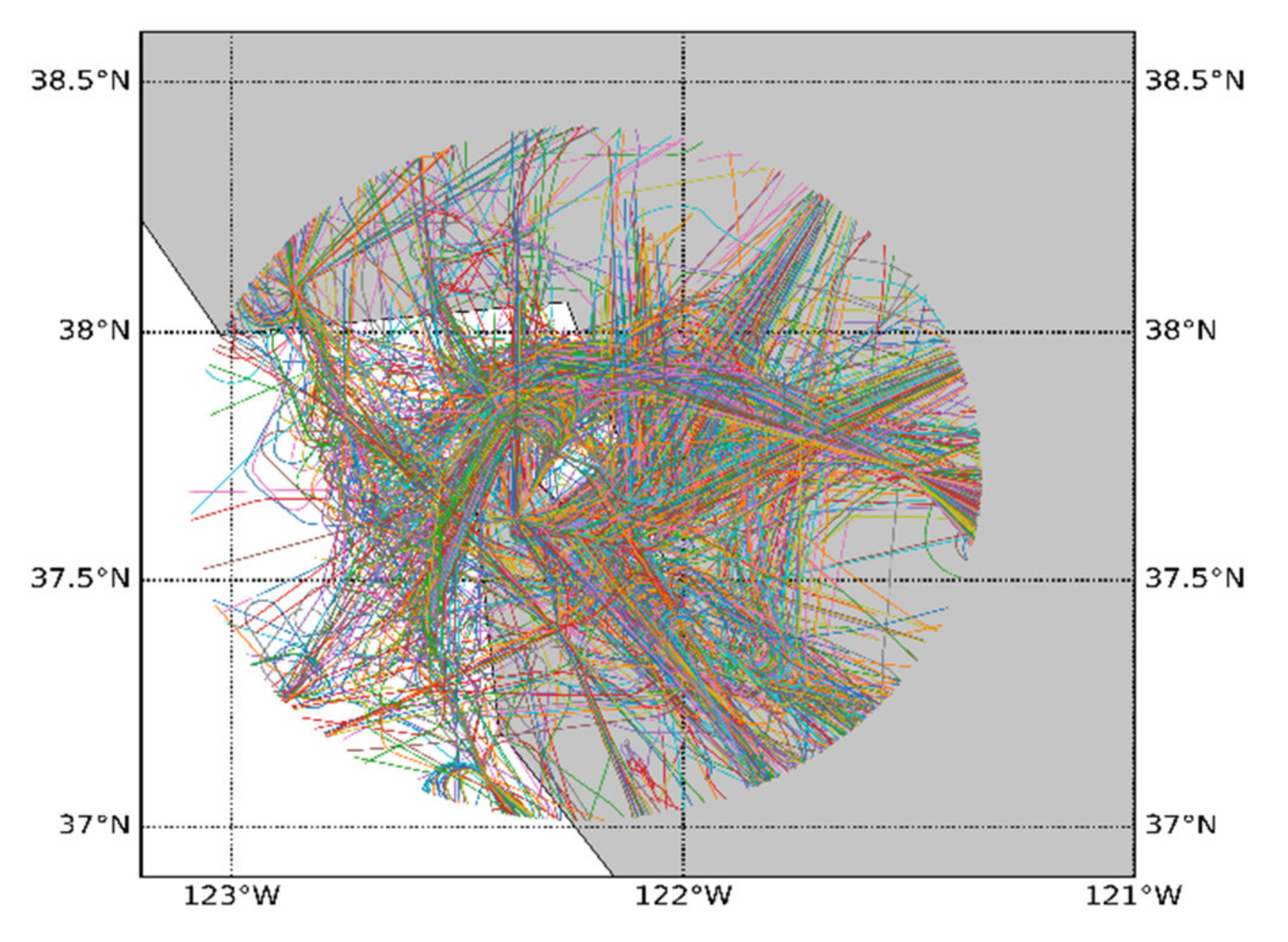
4.1. Data Processing

The flight trajectory data set used in this paper comes from the flight trajectory records over the San Francisco Bay Area from January to March 2006, as shown in Figure 5. This record covers the Northern California Terminal Radar Approach Control (NCT), which is a cylinder with a radius of 80 km and a height of 6000 m centered on Oakland International Airport (OAK). NCT includes three significant airports: Oakland Airport, San Francisco International Airport, San Jose International Airport, and many smaller airports. NCT is the fourth busiest terminal area in the United States, with an average of 133,000 flight instrument operations per month in 2006. The recorded data consist of the aircraft’s position (latitude, longitude, altitude), speed, and recording time. This paper only used the flight trajectory data in January 2006 as the data set to improve the training speed of the model. A preliminary quality analysis of the data set found that the proportion of duplicate records and records with missing attribute values was very small, so they were deleted directly. Then, the trajectory’s latitude, longitude and altitude data were converted into relative coordinates centered on OAK. According to the duration of the trajectory, it is found that the number of trajectory points varies from 10 to 550, and the time interval between two adjacent points is between 4 and 5 s. In order to facilitate multi-trajectory prediction, we first reconstructed the trajectory at a time interval of 5 s, and then determined the time stamp sequence with the reference time of 0:00 on 1 January 2006 and the interval of five seconds, and finally extracted the records corresponding to the previous timestamp sequence in all trajectories. In the end, 63,000 trajectories were obtained.
The minimum-maximum standardization method was used to standardize the trajectory data, and the data were mapped to [0, 1], eliminating the influence of different dimensions. Then, the standardized data were divided into a training set and a test set, where 70% of the trajectory data were used for training, and 30% were used for testing.

4.2. Evaluation Index

According to the suggestions in [63], the error indicators of the aircraft trajectory prediction experiment were determined: Mean Absolute Point-wise horizontal error (MAPHE), Mean Absolute Point-wise vertical error (MAPVE) and Mean Absolute Point-wise error (MAPE). Where PHE represents the distance between the 2D coordinates of each predicted point and the real coordinates; PVE represents the distance between the height of each predicted point and the real value; PE represents the distance between each predicted point and the real value. MAPHE, MAPVE, and MAPE, respectively, represent their average errors, as shown in Equations (9)–(11).
MAPHE = i = 1 N t = T o b s + 1 T p r e d ( x ^ t i x t i ) 2 + ( y ^ t i y t i ) 2 N ( T p r e d ( T o b s + 1 ) )
MAPVE = i = 1 N t = T o b s + 1 T p r e d ( z ^ t i z t i ) 2 N ( T p r e d ( T o b s + 1 ) )
MAPE = i = 1 N t = T o b s + 1 T p r e d ( x ^ t i x t i ) 2 + ( y ^ t i y t i ) 2 + ( z ^ t i z t i ) 2 N ( T p r e d ( T o b s + 1 ) )
where ( x t i , y t i , z t i ) represents the true 3D position of the i - th aircraft at time t , ( x ^ t i , y ^ t i , z ^ t i ) represents the corresponding predicted value, N represents the number of aircraft in the airspace, T o b s represents the length of the observation sequence of the trajectory, and T p r e d represents the length of the predicted sequence of the trajectory.

4.3. Parameter Setting

S-LSTM comprises multiple LSTM networks, so the model parameters are similar to LSTM networks, including structural parameters and internal parameters. The structural parameters include the sequence length l s e q , the number of hidden layers L , and the number of hidden layer neurons h n o d e . Compared with LSTM, S-LSTM also considers the number of neurons in the embedding layer e n o d e that combines the social hidden state with the position coordinates. The internal parameters include the size of each batch of training samples λ , the number of training iterations ε for all samples, the learning rate, and the weight parameters. Among them, the weight parameter was initialized by randomly assigning values in the interval [0, 1]. In the experiment, L was set to multiple, and it was found that the running time was greatly increased while the prediction accuracy was not improved much. Therefore, L was defaulted to 1 in order to simplify the model. Commonly used learning rates are 0.001, 0.01, 0.1, 0.003, 0.03, and 0.3, and commonly used decay rates are 0.85, 0.9, and 0.95, which are manually adjusted and selected based on experience during the experiment. Observe the relationship between the number of iterations and the loss during adjustment and find the initial learning rate and decay rate corresponding to the fastest loss reduction, which are 0.003 and 0.95, respectively. There is no universal determination rule for the remaining parameters. In this paper, the parameters were determined through Bayesian optimization. First of all, the value range of each parameter is determined: l s e q range was [20,25], h n o d e range was [64, 128], e n o d e range was [16, 64], λ range was [20,60], and ε range was [50, 100]. Then, the maximum number of evaluations for Bayesian optimization was set to 100, that is, 100 parameter combinations were generated from each parameter range, and the parameter combination that minimized the prediction error of the test set was selected as the optimal parameter combination. In addition to the above basic parameters, the S-LSTM model also considers the neighborhood size δ and the social pool merge window size N 0 mentioned in the social pool in the previous section. Since the aircraft trajectory is a collection of 3D space coordinates, δ was divided into a horizontal range and a vertical range, which were set to 4000 and 800, respectively. This meant that other aircraft within 2000 m in front of the aircraft and 400 m up and down were considered. Additionally, N 0 was set to 2. At the same time, the average aircraft density per second in the data set was 50. The data set in this paper was assumed to be able to predict up to 50 aircraft trajectories at the same time. Finally, the RMSprop algorithm was utilized to train the model. The parameters of S-LSTM are shown in Table 1.

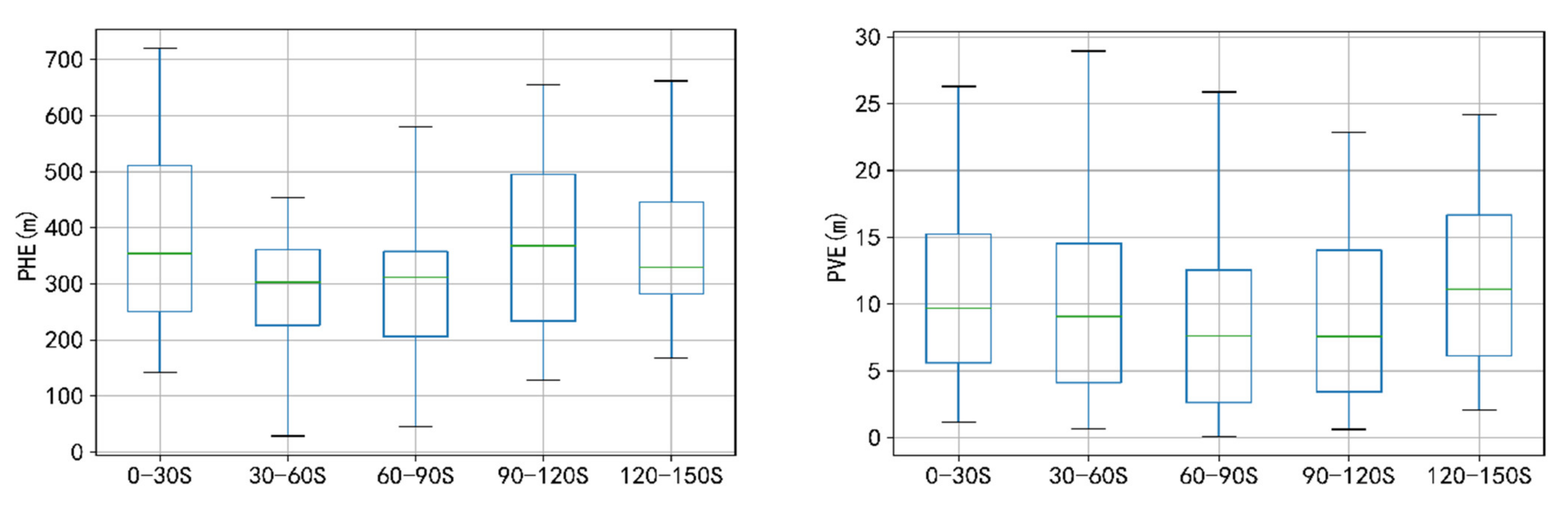
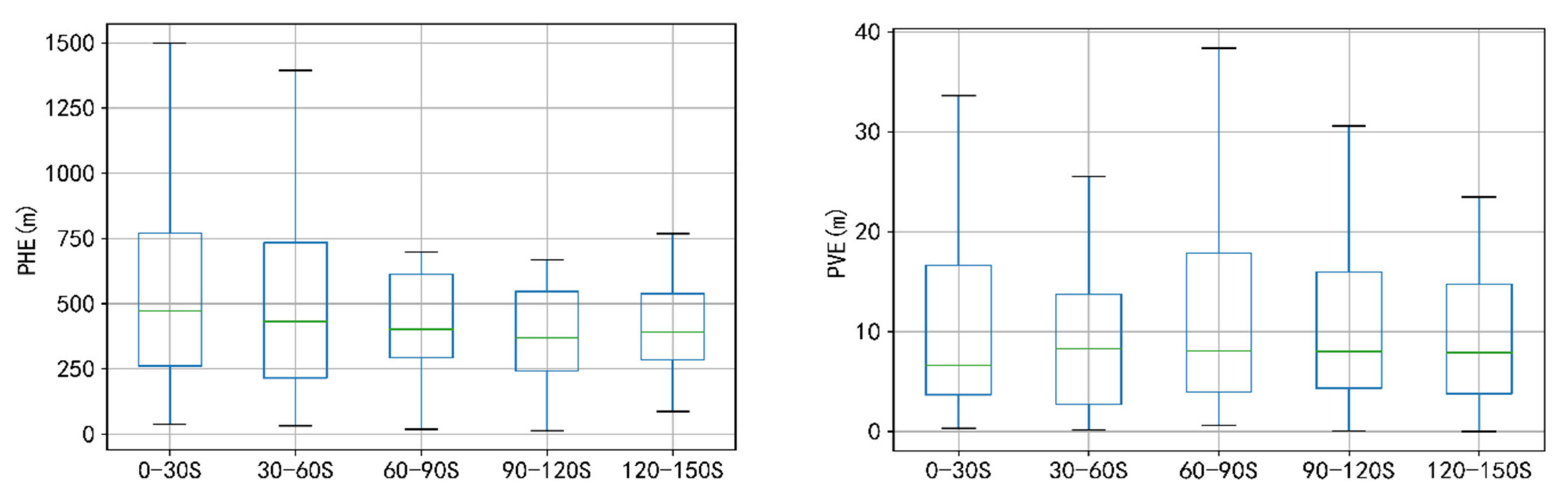
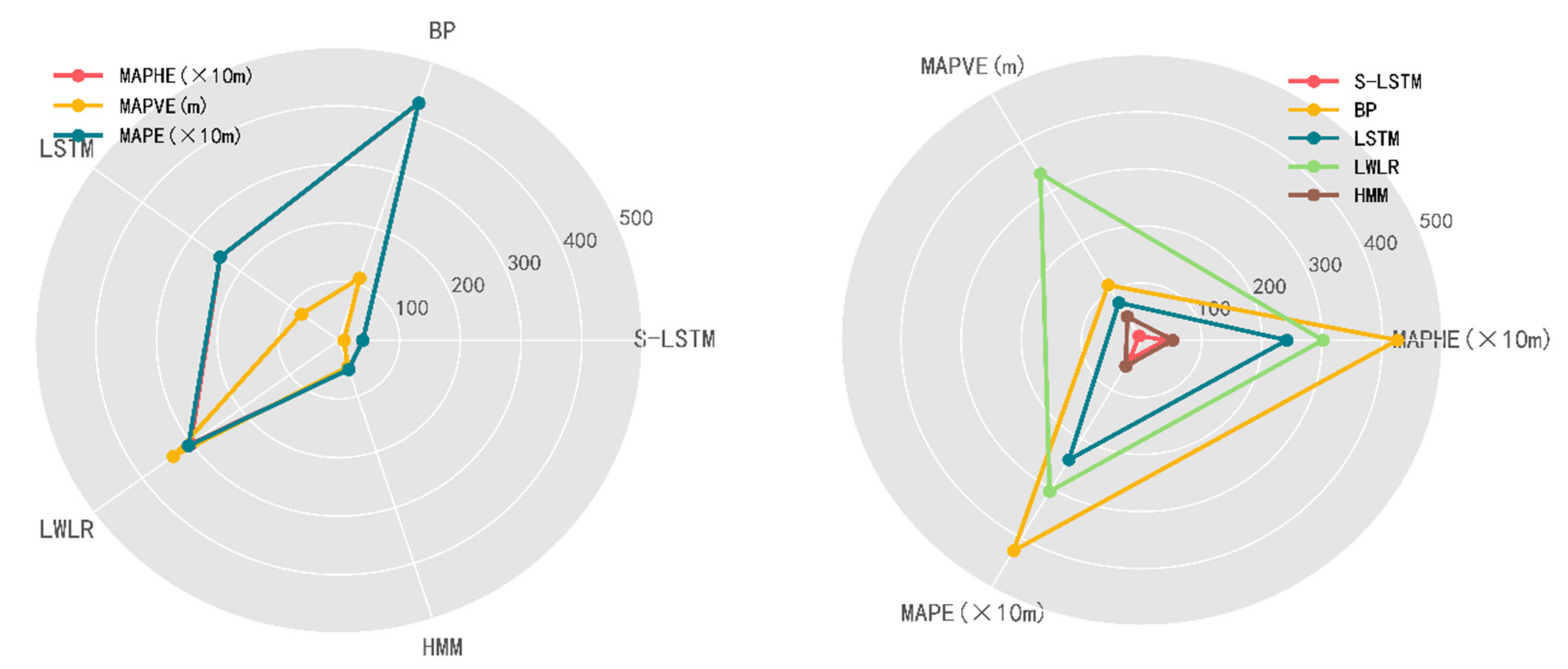
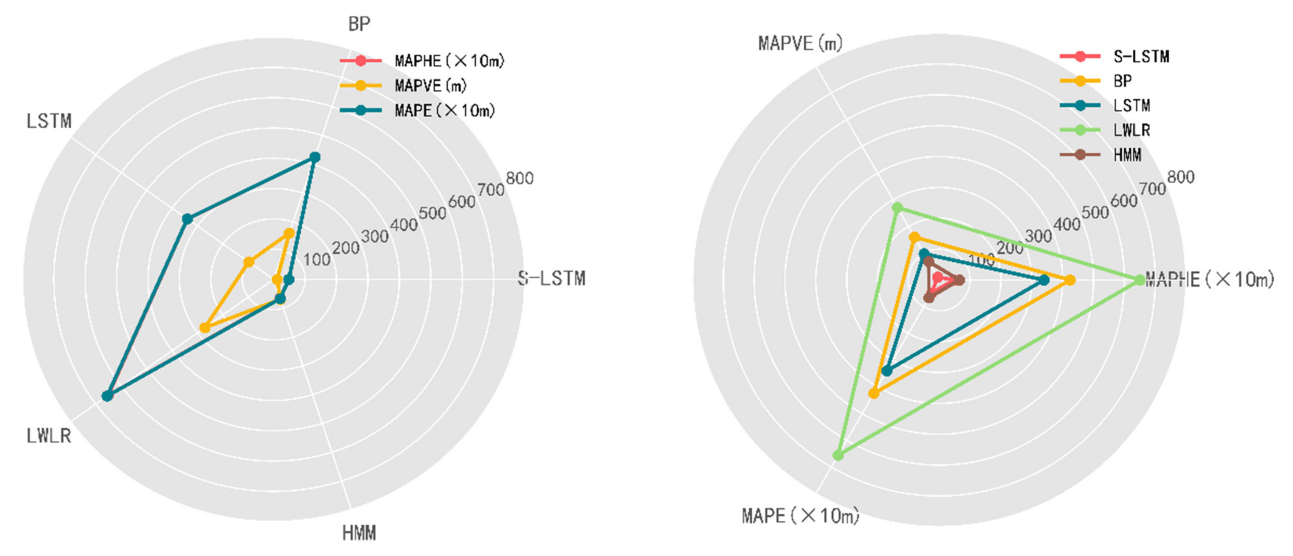
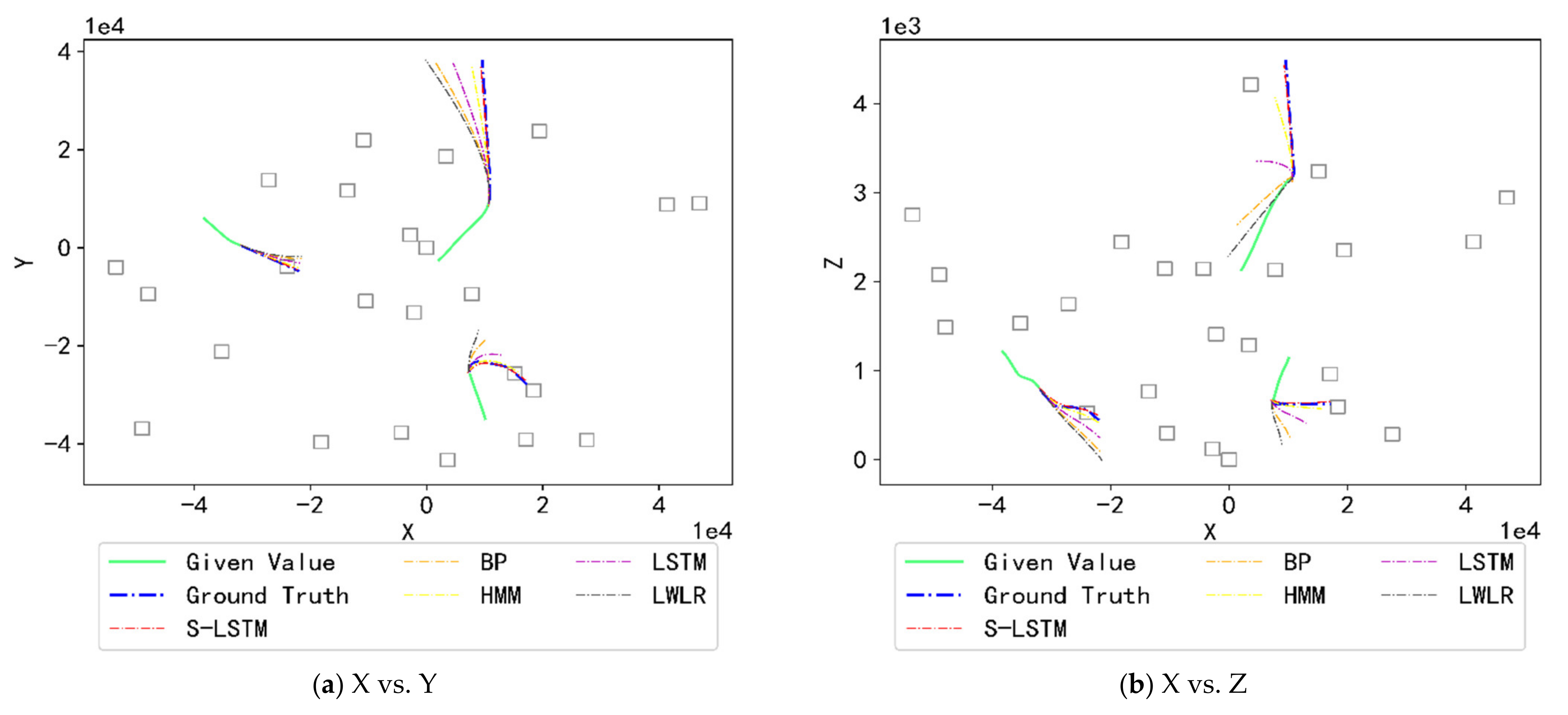
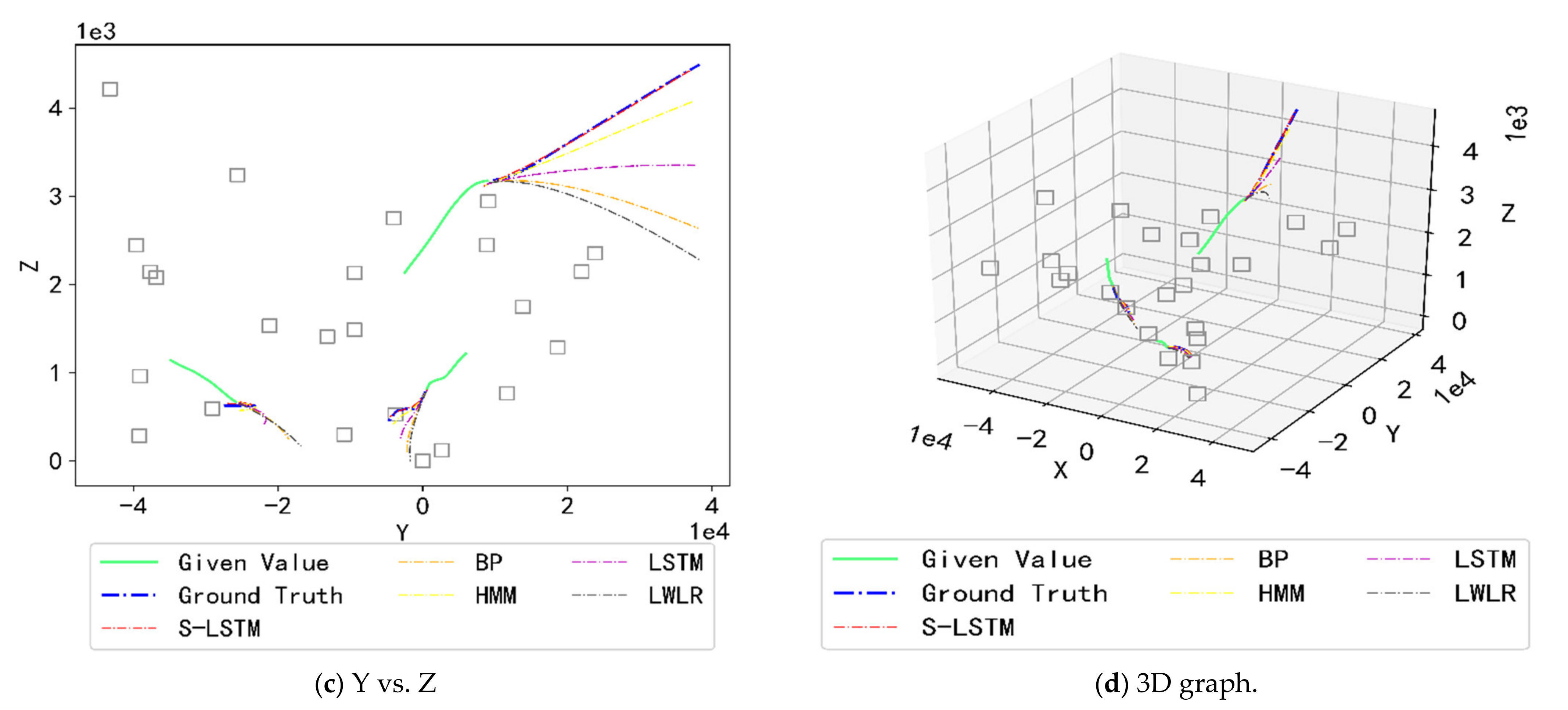
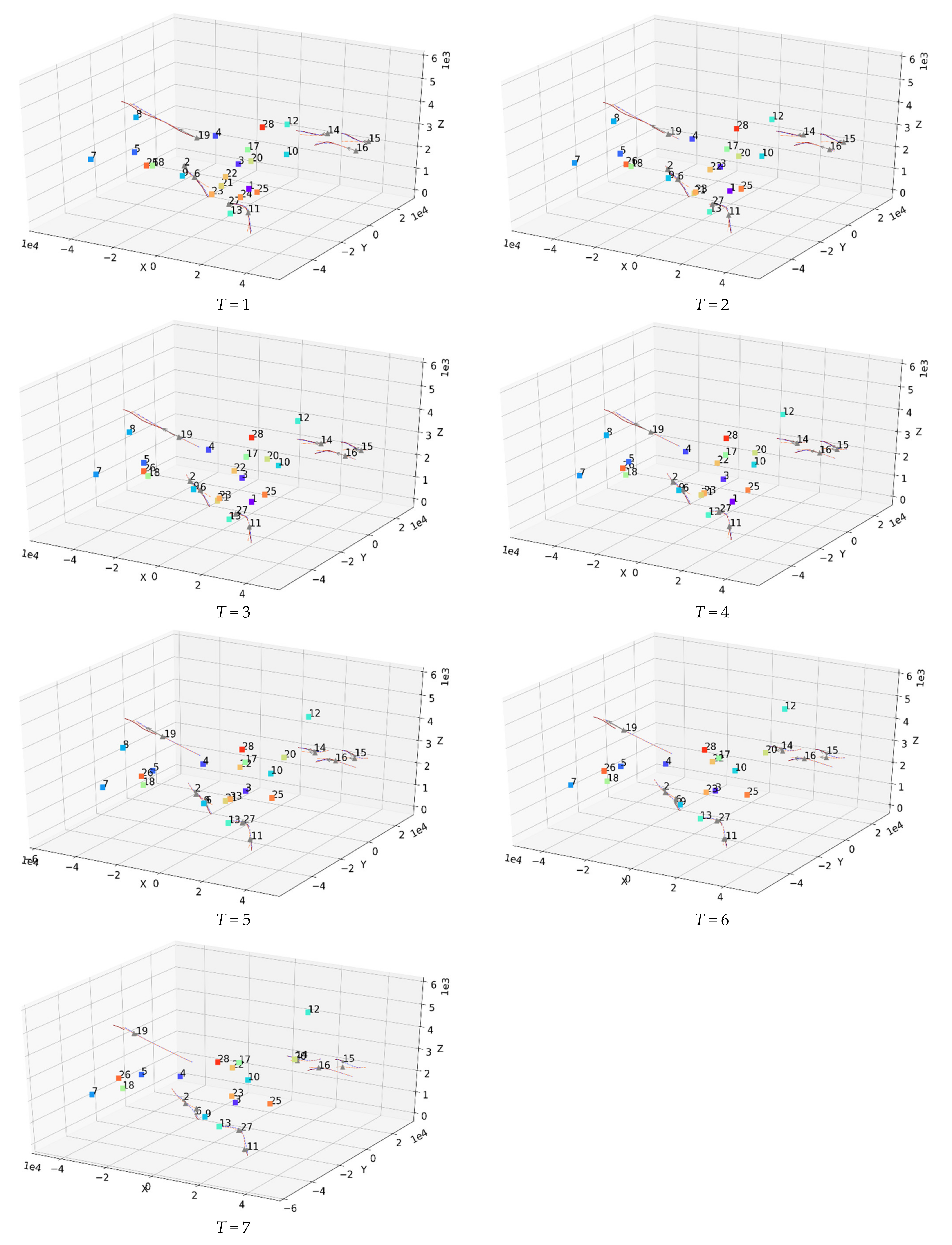
4.4. Model Performance Analysis

In this section, the evaluation indicators were used to analyze the performance of the trained S-LSTM prediction model on the test set. In the experiment, given the data of the first 100 s of the flight trajectory, predict the trajectory sequence of the next 150 s, that is, the length of the observation sequence is 20 and the length of the predicted sequence is 30. According to the predicted value of each trajectory output by the model, the three types of error values were calculated for each trajectory point and the prediction accuracy and robustness of the arrival and departure flights in different time intervals were observed. Due to the different operating characteristics of arrival and departure flights in the terminal area, they are discussed here separately and take 30 s as the time interval for statistics, that is, the results will be displayed in five boxes, as shown in Figure 6 and Figure 7.
Figure 6 is a box plot of PHE and PVE for arrival flights. From the box plot of PHE, it can be seen that the average error of all trajectory points in each time interval is within the range of 300 to 400 m, the maximum error does not exceed 750 m, the minimum error does not exceed 200 m, the average error reaches the maximum in 90 to 120 s, and the overall change is small. The upper and lower limits of PHE are the smallest in 30 to 60 s, but they do not change much as the time interval changes. From the box plot of PVE, it can be seen that the average error of all trajectory points in each time interval is within the range of 5 to 12 m, the maximum error does not exceed 30 m, the minimum error does not exceed 5 m, the average error reaches the maximum in 120 to 150 s, and the overall change is relatively stable. Similar to PHE, the upper and lower limits of PVE do not change much as the time interval changes, and it reaches the minimum in 120 to 150 s. Due to the overall small PVE error, the box plot of PE is similar to PHE, so it will not be shown here. The analysis shows that the average error change range is small and the upper and lower limits of each time interval also change little whether in the horizontal or vertical direction. It proves that our model can effectively avoid the rapid propagation of errors over time, so as to improve the accuracy and stability of inbound flight forecasts.
Figure 7 is a box plot of PHE and PVE for departure flights. From the box plot of PHE, it can be seen that the average error of all trajectory points in each time interval is within the range of 270 to 500 m, the maximum error does not exceed 1500 m, the minimum error does not exceed 120 m, the average error reaches the maximum in 0 to 30 s, and the overall change is small. The upper and lower limits of PHE are the smallest in 90 to 120 s. After 60 s, the upper and lower limits tend to be stable as the time interval changes. From the box plot of PVE, it can be seen that the average error of all trajectory points in each time interval is within the range of 5 to 10 m, the maximum error does not exceed 40 m, the minimum error does not exceed 5 m, the average error reaches the maximum in 30 to 60 s, and the overall change is very stable. Unlike PHE, the upper and lower limits of PVE do not change much as the time interval changes, and it reaches the minimum in 120 to 150 s. The analysis shows that the average error changes relatively smoothly whether in the horizontal or vertical direction, similar to the arrival flight. However, the difference is that the upper and lower limits change more steadily in the vertical direction than in the horizontal direction as the time interval changes. It proves that our model can improve departure flights prediction performance as time changes, but stability needs to be improved.
Through calculation, the MAPHE of arrival flights is about 364 m and the MAPVE is about 11 m, while the MAPHE of departure flights is about 730 m and the MAPVE is about 13 m. Comparing the overall average error of arrival and departure flights, it is found that the error of the latter is greater than that of the former, no matter whether it is in the horizontal or vertical direction. Comparing Figure 6 and Figure 7, it is also found that the upper and lower limits of the overall error of departure flights are larger than those of arrival flights, indicating that the model has better stability and robustness for predicting the arrival trajectory. Therefore, the prediction effect of our model on arrival flights is better than on departure flights.
This experiment compares this model with LWLR, HMM, BP NN, and LSTM proposed in the current trajectory prediction research to verify the performance of the model in this paper. For the same trajectory data set, all models use the same training set and test set for parameter setting and model training. MAPHE, MAPVE and MAPE are used as evaluation indicators and 0 to 30 s is selected as the time interval to evaluate the performance of each model. The specific results are shown in Figure 8 and Figure 9, respectively, showing the comparison of prediction error for the arrival and departure flights.
It can be found from Figure 8 that for arrival flights, LWLR has the worst prediction effect in the horizontal direction, BP NN is slightly better than LWLR, and BP NN is the worst in the vertical direction, and LWLR is slightly better than BP NN. In general, the prediction effects of these two methods are not good, and the LSTM model is better than them in the horizontal and vertical directions, which proves that the LSTM model has certain advantages in trajectory prediction and can fully consider time dependence. At the same time, the prediction accuracy of LSTM is lower than that of HMM, possibly because HMM is more suitable for short-term prediction of arrival flights than LSTM. Finally, it is found that the S-LSTM proposed in this paper can further improve the prediction accuracy compared with HMM. It reduces the error by about 40% in the horizontal direction and about 8% in the vertical direction. This may be due to its consideration of the interactive influence of the surrounding aircraft trajectory rather than its own trajectory.
It can be found from Figure 9 that for departure flights, the prediction effect of LWLR is the worst in both horizontal and vertical directions. Although BP NN is better than LWLR, the prediction effect is still not ideal, which is similar to the prediction result of arrival flights. Similarly, the prediction accuracy of LSTM is higher than the previous two methods, but it is significantly lower than HMM. Compared with HMM, the S-LSTM proposed in this paper can further improve the prediction accuracy, and the error is reduced by about 35% in the horizontal direction and about 6% in the vertical direction. Therefore, the model in this paper is significantly better than others in the prediction effect of arrival and departure flights. At the same time, compared with Figure 8, the prediction results of the departure flights in Figure 9 show that the overall error in the horizontal and vertical directions is larger than that of arrival flights. Therefore, our model is more suitable for predicting the 4D trajectory of arrival flights than departure flights.
Next, this paper randomly selects the prediction results of three trajectories in the airspace over a period from the test set to visualize and predicts the 3D trajectory in the future 150 s. Figure 10a shows the prediction results of trajectories from a horizontal perspective. It can be found that S-LSTM fits well on the three trajectories, while other models have poor fitting effect on the trajectory with larger steering during flight. Figure 10b,c shows the prediction results from a vertical perspective. Spatial coordinates are used to display the trajectory for clarity, as shown in Figure 10d, and the gray boxes in the figure represent other aircraft in the airspace. Similarly, S-LSTM has a better fitting effect than other models and can capture the steady climb or decline of the trajectory well, avoiding aircraft that may collide.

4.5. Discussion of Results

A suitable airspace scene is selected to visually analyze and discuss the prediction results to verify whether S-LSTM considers the interaction between aircraft in the airspace. Here, only representative trajectories are selected in the airspace to display their trajectories for clarity of visualization. The visualization results are shown in Figure 11. They, respectively, show the real-time position and representative trajectory of the aircraft at seven times. A gray triangle represents the representative aircraft in the figure, and the solid red line represents the actual trajectory of the corresponding aircraft. The blue dotted line represents the predicted value using S-LSTM, the orange dotted line represents the predicted value using LSTM, and other aircraft are represented by squares.
In Figure 11, at time T = 1 , there are 28 aircraft in the airspace (numbered from 1 to 28, respectively). However, aircraft continue to leave the airspace over time. Aircraft No. 24 left the airspace at time T = 2 , aircraft No. 1 left at time T = 5 , and No. 8 and No. 21 left at time T = 6 . In the end, eight aircrafts of No. 2, No. 6, No. 14, No. 15, No. 16, No. 11, No. 19, and No. 27 are selected to show their trajectories. At time T = 1 , according to the real trajectory, No. 2 is an arrival flight, and its trajectory is basically the same as No. 6 ahead of it. No. 27 may interact with No. 11. No. 14 may affect No. 15 and No. 16 at the same time, and No. 16 may affect No. 15. At this time, there is no aircraft that may affect No. 19 in the airspace in front of it. From T = 2 to T = 7 , according to the prediction result of S-LSTM, No. 2 began to descend gently, which can effectively avoid collision with No. 6 during the descent. No. 27 slowed down the turning speed and descent speed, reducing the risk of collision with No. 11. No. 15 climbed up to avoid collisions with No. 14 ahead and No. 16 at the front and bottom, and No. 16 gradually descended to avoid collisions with No. 14 ahead and above. In contrast, the prediction results of LSTM did not take into account the potential impact of the surrounding aircraft. No. 2 still followed the downward trend of the trajectory at time T = 1 , resulting in a steep decline, which is likely to collide with No. 6. No. 27 did not slow down the speed during the turning and descent stage, which may have an impact on the descent process of No. 11. No. 15 was still falling according to the original trend, and may conflict with No. 16, while No. 16 was still rising and may conflict with No. 14.
Table 2 further lists the errors of the representative trajectories in Figure 11 under the two prediction models. In general, the trajectories of aircraft No. 2, 27, 15 and 16 predicted by LSTM are quite different from S-LSTM, while the prediction error of aircraft No. 19 is relatively small. This indirectly reflects that our model can significantly improve prediction accuracy when predicting aircraft trajectories affected by other aircraft. Still, when predicting unaffected aircraft trajectories, our model’s prediction effect is the same as LSTM.
Different types of flight trajectory data are input in S-LSTM to predict and calculate the prediction errors to investigate whether there is an interaction between the arrival and departure flights of several major airports in NCT. The results are shown in Table 3. When only the arrival flights data are input, the average error in the horizontal direction is 690 m and the vertical direction is 12 m. When only the departure flights data are input, the horizontal direction is 762 m and the vertical direction is 23 m. However, if all flights data are input at the same time, the average error of arrival flights trajectory in the horizontal direction is reduced by 38 m, the vertical direction is reduced by 4 m, departure flights is reduced by 87 m in the horizontal direction, and the vertical direction is reduced by 6 m. It can be seen that the arrivals and departures of major airports in this airspace interact with each other.

5. Conclusions

This paper proposes the use of S-LSTM to predict multiple aircraft trajectories simultaneously. Different from other trajectory prediction models, this model considers the interaction between trajectories and breaks through the limitations of single aircraft trajectory prediction. In the modeling process, an LSTM network was first established for each aircraft in the control area, and the pooling layer was used to integrate the hidden state output of the LSTM network associated with the aircraft. Then, the integrated social hidden state, trajectory information, and its own hidden state were used as the input of the next time step of the network, and the model was trained by maximizing the probability of the output trajectory. In trajectory generation, the model used the predicted value at the previous moment to replace the real value to predict the trajectory at the current moment and iterated until the entire trajectories were generated.
In the case analysis, box plots were used to calculate the prediction errors of arrival and departure flights in different time intervals, and it was analyzed that when using our model to predict in the selected NCT, arrival flights were better than departure flights in terms of prediction accuracy and stability. At the same time, the radar chart was used to compare the prediction errors of arrival and departure flights under S-LSTM and four typical trajectory prediction models. The results showed that the prediction effect of our model was better than other comparison models, whether it was arrival or departure. Additionally, the error of arrival flights was smaller than that of departure flights, indicating that our model was more suitable for predicting the 4D trajectory of the arrival flights in NCT.
A suitable airspace scene was also selected to visually analyze and the prediction results were discussed during the experiment, which showed that our model can indeed effectively utilize the interaction between aircraft. In addition, the trajectory data of the arrival and departure flights were separately input into the model to predict, and it was found that the arrival and departure of the main airports in NCT were mutually affected.
In addition to the above conclusions, there are still some areas worthy of further improvement and perfection. The model in this paper only uses trajectory information such as longitude, latitude, altitude, speed and angle, without considering the impact of high altitude meteorological conditions in actual operations. Therefore, the future research work of multi-aircraft trajectory prediction can further consider how to integrate the meteorological conditions around the aircraft into the prediction model to achieve more accurate and stable trajectory prediction. In addition, the pooling layer is used to select other aircraft that may interact with each other around the aircraft in this study. At present, the popular element attention mechanism in neural networks is also used to complete similar tasks, making the neural network focus on processing a small part of the useful information in a large amount of input information, and ignore other information. Therefore, we can consider using the attention mechanism to improve the S-LSTM network in future research.

Author Contributions

Conceptualization, Z.X., W.Z., X.C. and P.C.; Methodology, Z.X. and W.Z.; Investigation, Z.X., X.C. and P.C.; Data curation, Z.X., X.C. and P.C.; Supervision, Z.X. and W.Z.; Validation, Z.X.; Writing—original draft preparation, Z.X.; Writing—review and editing, Z.X., W.Z., X.C. and P.C. All authors have read and agreed to the published version of the manuscript.

Funding

This research was funded by the National Natural Science Foundation of China (Grant No.62076126), the Fundamental Research Funds for the Central Universities (Grant NS2018044) and the Graduate Open Funds of NUAA (Grant kfjj20200718).

Institutional Review Board Statement

Not applicable.

Informed Consent Statement

Not applicable.

Data Availability Statement

Not applicable.

Acknowledgments

We would like to thank the National Air Traffic Control Flight Flow Management Technology Key Laboratory of Nanjing University of Aeronautics and Astronautics for providing the ADS-B data used in the model tests described in this paper.

Conflicts of Interest

The authors declare no conflict of interest.

References

  1. Joint Planning And Development Office. Concept of Operations for the Next Generation Air Transportation System; Joint Planning and Development Office: Washington, DC, USA, 2007. [Google Scholar]
  2. Undertaking, S.J. The European ATM Master Plan, Edition 2, October 2012. Available online: https://www.atmmasterplan.eu/download/25 (accessed on 30 October 2012).
  3. Li, X.; Peng, L.; Yao, X.; Cui, S.; Hu, Y.; You, C.; Chi, T. Long short-term memory neural network for air pollutant concentration predictions: Method development and evaluation. Environ. Pollut. 2017, 231, 997–1004. [Google Scholar] [CrossRef]
  4. Fischer, T.; Krauss, C. Deep learning with long short-term memory networks for financial market predictions. Eur. J. Oper. Res. 2018, 270, 654–669. [Google Scholar] [CrossRef] [Green Version]
  5. Yang, B.; Sun, S.; Li, J.; Lin, X.; Tian, Y. Traffic flow prediction using LSTM with feature enhancement. Neurocomputing 2019, 332, 320–327. [Google Scholar] [CrossRef]
  6. Zeng, W.; Quan, Z.; Zhao, Z.; Xie, C.; Lu, X. A deep learning approach for aircraft trajectory prediction in terminal airspace. IEEE Access 2020, 8, 151250–151266. [Google Scholar] [CrossRef]
  7. Chatterji, G. Short-term trajectory prediction methods. In Proceedings of the Guidance, Navigation, and Control Conference and Exhibit, Portland, OR, USA, 9–11 August 1999; p. 4233. [Google Scholar]
  8. Avanzini, G. Frenet-based algorithm for trajectory prediction. J. Guid. Control. Dynam. 2004, 27, 127–135. [Google Scholar] [CrossRef]
  9. Lymperopoulos, I.; Lygeros, J. Sequential Monte Carlo methods for multi-aircraft trajectory prediction in air traffic management. Int. J. Adapt. Control Signal Process. 2010, 24, 830–849. [Google Scholar] [CrossRef]
  10. Choi, P.P.; Hebert, M. Learning and predicting moving object trajectory: A piecewise trajectory segment approach. Robot. Inst. 2006, 337, 1–17. [Google Scholar]
  11. Ayhan, S.; Samet, H. Aircraft trajectory prediction made easy with predictive analytics. In Proceedings of the 22nd ACM SIGKDD International Conference on Knowledge Discovery and Data Mining, San Francisco, CA, USA, 14–19 August 2016; pp. 21–30. [Google Scholar]
  12. Lin, Y.; Zhang, J.-W.; Liu, H. An algorithm for trajectory prediction of flight plan based on relative motion between positions. Front. Inf. Technol. Electron. Eng. 2018, 19, 905–916. [Google Scholar] [CrossRef]
  13. Lin, Y.; Yang, B.; Zhang, J.; Liu, H. Approach for 4-d trajectory management based on HMM and trajectory similarity. J. Mar. Sci. Technol. 2019, 27, 246–256. [Google Scholar]
  14. Rezaie, R.; Li, X.R. Trajectory modeling and prediction with waypoint information using a conditionally Markov sequence. In Proceedings of the 2018 56th Annual Allerton Conference on Communication, Control, and Computing, Champaign, IL, USA, 2–5 October 2018; pp. 486–493. [Google Scholar]
  15. Bar-Shalom, Y.; Li, X.R.; Kirubarajan, T. Estimation with Applications to Tracking and Navigation: Theory Algorithms and Software; John Wiley & Sons: Hoboken, NJ, USA, 2004. [Google Scholar]
  16. Yepes, J.L.; Hwang, I.; Rotea, M. New algorithms for aircraft intent inference and trajectory prediction. J. Guid. Control Dynam. 2007, 30, 370–382. [Google Scholar] [CrossRef]
  17. Jun-feng, Z.; Xiao-guang, W.; Fei, W. Aircraft trajectory prediction based on modified interacting multiple model algorithm. J. Donghua Univ. 2015, 180–184. [Google Scholar]
  18. Xi, L.; Jun, Z.; Yanbo, Z.; Wei, L. Simulation study of algorithms for aircraft trajectory prediction based on ADS-B technology. In Proceedings of the 2008 Asia Simulation Conference-7th International Conference on System Simulation and Scientific Computing, Beijing, China, 10–12 October 2008; pp. 322–327. [Google Scholar]
  19. Liu, Y.; Li, X.R. Intent based trajectory prediction by multiple model prediction and smoothing. In Proceedings of the AIAA Guidance, Navigation, and Control Conference, Kissimmee, FL, USA, 5–9 January 2015; p. 1324. [Google Scholar]
  20. Seah, C.E.; Hwang, I. A hybrid estimation algorithm for terminal-area aircraft tracking. In Proceedings of the AIAA Guidance, Navigation and Control Conference and Exhibit, Hilton Head, SC, USA, 20–23 August 2007; p. 6691. [Google Scholar]
  21. Seah, C.E.; Hwang, I. Terminal-area aircraft tracking using hybrid estimation. J. Guid. Control Dynam. 2009, 32, 836–849. [Google Scholar] [CrossRef]
  22. Hwang, I.; Seah, C.E. Intent-based probabilistic conflict detection for the next generation air transportation system. In Proceedings of the IEEE, Beijing, China, 2–5 November 2008; Volume 96, pp. 2040–2059. [Google Scholar]
  23. Liu, W.; Hwang, I. Probabilistic trajectory prediction and conflict detection for air traffic control. J. Guid. Control Dynam. 2011, 34, 1779–1789. [Google Scholar] [CrossRef]
  24. Fukuda, Y.; Shirakawa, M.; Senoguchi, A. Development and evaluation of trajectory prediction model. In Proceedings of the Proceedings of the 27th International Congress of the Aeronautical Sciences, Nice, France, 19–24 September 2010. [Google Scholar]
  25. Schuster, W. Trajectory prediction for future air traffic management–complex manoeuvres and taxiing. Aeronaut. J. 2015, 119, 121–143. [Google Scholar] [CrossRef] [Green Version]
  26. Zhang, J.; Liu, J.; Hu, R.; Zhu, H. Online four dimensional trajectory prediction method based on aircraft intent updating. Aerosp. Sci. Technol. 2018, 77, 774–787. [Google Scholar] [CrossRef]
  27. Lymperopoulos, I.; Lygeros, J.; Lecchini, A. Model based aircraft trajectory prediction during takeoff. In Proceedings of the AIAA Guidance, Navigation, and Control Conference and Exhibit, Keystone, CO, USA, 21–24 August 2006; p. 6098. [Google Scholar]
  28. Tang, X.-M.; Han, Y.-X. 4D trajectory estimation for air traffic control automation system based on hybrid system theory. PROMET-ZAGREB 2012, 24, 91–98. [Google Scholar] [CrossRef]
  29. Lee, J.; Lee, S.; Hwang, I. Hybrid System Modeling and Estimation for Arrival Time Prediction in Terminal Airspace. J. Guid. Control Dynam. 2016, 39, 903–910. [Google Scholar] [CrossRef]
  30. Félix, F.A.N.; Ruiz, M.A.V.; Querejeta, C.; Gallo, E.; Leonés, J.L. Predicting Aircraft Trajectory. Patent No. 9,020,662, 28 April 2015. [Google Scholar]
  31. Schuster, W.; Ochieng, W.; Porretta, M. High-performance trajectory prediction for civil aircraft. In Proceedings of the 29th Digital Avionics Systems Conference, Salt Lake City, UT, USA, 3–7 October 2010. [Google Scholar]
  32. Schuster, W.; Porretta, M.; Ochieng, W. High-accuracy four-dimensional trajectory prediction for civil aircraft. Aeronaut. J. 2012, 116, 45–66. [Google Scholar] [CrossRef] [Green Version]
  33. Porretta, M.; Dupuy, M.-D.; Schuster, W.; Majumdar, A.; Ochieng, W. Performance evaluation of a novel 4D trajectory prediction model for civil aircraft. J. Navig. 2008, 61, 393. [Google Scholar] [CrossRef]
  34. Thipphavong, D.P.; Schultz, C.A.; Lee, A.G.; Chan, S.H. Adaptive algorithm to improve trajectory prediction accuracy of climbing aircraft. J. Guid. Control Dynam. 2013, 36, 15–24. [Google Scholar] [CrossRef] [Green Version]
  35. Baklacioglu, T.; Cavcar, M. Aero-propulsive modelling for climb and descent trajectory prediction of transport aircraft using genetic algorithms. Aeronaut. J. 2014, 118, 65–79. [Google Scholar] [CrossRef]
  36. De Leege, A.; van Paassen, M.; Mulder, M. A machine learning approach to trajectory prediction. In Proceedings of the AIAA Guidance, Navigation, and Control (GNC) Conference, Boston, MA, USA, 19–22 August 2013; p. 4782. [Google Scholar]
  37. Hamed, M.G.; Gianazza, D.; Serrurier, M.; Durand, N. Statistical prediction of aircraft trajectory: Regression methods vs point-mass model. In Proceedings of the ATM Seminar, Chicago, IL, USA, 10–13 June 2013. [Google Scholar]
  38. Tastambekov, K.; Puechmorel, S.; Delahaye, D.; Rabut, C. Aircraft trajectory forecasting using local functional regression in Sobolev space. Transp. Res. Part C Emerg. Technol. 2014, 39, 1–22. [Google Scholar] [CrossRef] [Green Version]
  39. Le Fablec, Y.; Alliot, J.-M. Using Neural Networks to Predict Aircraft Trajectories. In Proceedings of the IC-AI, Las Vegas, NV, USA, 28 June–1 July 1999; pp. 524–529. [Google Scholar]
  40. Shi, Z.; Xu, M.; Pan, Q.; Yan, B.; Zhang, H. LSTM-based flight trajectory prediction. In Proceedings of the 2018 International Joint Conference on Neural Networks (IJCNN), Rio de Janeiro, Brazil, 8–13 July 2018; pp. 1–8. [Google Scholar]
  41. Fernando, T.; Denman, S.; McFadyen, A.; Sridharan, S.; Fookes, C. Tree memory networks for modelling long-term temporal dependencies. Neurocomputing 2018, 304, 64–81. [Google Scholar] [CrossRef] [Green Version]
  42. Ma, Z.; Yao, M.; Hong, T.; Li, B. Aircraft surface trajectory prediction method based on lstm with attenuated memory window. J. Phys. Conf. Ser. 2019, 1215, 012003. [Google Scholar] [CrossRef]
  43. Liu, Y.; Hansen, M.; Lovell, D.J.; Chuang, C.; Ball, M.O.; Gulding, J. Causal analysis of en route flight inefficiency-the US experience. In Proceedings of the Twelfth USA/Europe Air Traffic Management Research and Development Seminar, Seattle, WA, USA, 27–30 June 2017. [Google Scholar]
  44. Pang, Y.; Xu, N.; Liu, Y. Aircraft trajectory prediction using LSTM neural network with embedded convolutional layer. In Proceedings of the Annual Conference of the PHM Society, Scottsdale, AZ, USA, 21–26 September 2019. [Google Scholar]
  45. Wu, Z.-J.; Tian, S.; Ma, L. A 4D trajectory prediction model based on the BP neural network. J. Intell. Syst. 2019, 29, 1545–1557. [Google Scholar] [CrossRef]
  46. Han, P.; Yue, J.; Fang, C.; Shi, Q.; Yang, J. Short-term 4D trajectory prediction based on LSTM neural network. In Proceedings of the Second Target Recognition and Artificial Intelligence Summit Forum, Shenyang, China, 28–30 August 2020; p. 114270M. [Google Scholar]
  47. Zhang, X.; Mahadevan, S. Bayesian neural networks for flight trajectory prediction and safety assessment. Decis. Support. Syst. 2020, 131, 113246. [Google Scholar] [CrossRef]
  48. Pang, Y.; Liu, Y. Probabilistic aircraft trajectory prediction considering weather uncertainties using dropout as bayesian approximate variational inference. In Proceedings of the AIAA Scitech 2020 Forum, Orlando, FL, USA, 6–10 January 2020; p. 1413. [Google Scholar]
  49. Pang, Y.; Liu, Y. Conditional Generative Adversarial Networks (CGAN) for Aircraft Trajectory Prediction considering weather effects. In Proceedings of the AIAA Scitech 2020 Forum, Orlando, FL, USA, 6–10 January 2020; p. 1853. [Google Scholar]
  50. Wang, Z.; Liang, M.; Delahaye, D. Short-term 4d trajectory prediction using machine learning methods. In Proceedings of the SESAR Innovation Days, Belgrade, Serbia, 28–30 November 2017; pp. 1–10. [Google Scholar]
  51. Wang, Z.; Liang, M.; Delahaye, D. A hybrid machine learning model for short-term estimated time of arrival prediction in terminal manoeuvring area. Transp. Res. Part C Emerg. Technol. 2018, 95, 280–294. [Google Scholar] [CrossRef]
  52. Georgiou, H.; Pelekis, N.; Sideridis, S.; Scarlatti, D.; Theodoridis, Y. Semantic-aware aircraft trajectory prediction using flight plans. Int. J. Data Sci. Anal. 2020, 9, 215–228. [Google Scholar] [CrossRef]
  53. Hamed, M.G. Méthodes Non-Paramétriques Pour la Prévision D’intervalles Avec Haut Niveau de Confiance: Application à la Prévision de Trajectoires D’avions. Ph.D. Thesis, Institut National Polytechnique de Toulouse-INPT, Toulouse, France, 2014. [Google Scholar]
  54. Shen, Z.; Tang, X. A Novel 4D track prediction approach combining empirical mode decomposition with nonlinear correlation coefficient. In Proceedings of the 15th COTA International Conference of Transportation Professionals, Beijing, China, 24–27 July 2015; pp. 25–34. [Google Scholar]
  55. Gallego, C.E.V.; Comendador, V.F.G.; Carmona, M.A.A.; Valdés, R.M.A.; Nieto, F.J.S.; Martínez, M.G. A machine learning approach to air traffic interdependency modelling and its application to trajectory prediction. Transp. Res. Part C Emerg. Technol. 2019, 107, 356–386. [Google Scholar] [CrossRef]
  56. Tang, X.; Chen, P.; Zhang, Y. 4D trajectory estimation based on nominal flight profile extraction and airway meteorological forecast revision. Aerosp. Sci. Technol. 2015, 45, 387–397. [Google Scholar] [CrossRef]
  57. Fernández, E.C.; Cordero, J.M.; Vouros, G.; Pelekis, N.; Kravaris, T.; Georgiou, H.; Fuchs, G.; Andrienko, N.; Andrienko, G.; Casado, E. DART: A machine-learning approach to trajectory prediction and demand-capacity balancing. In Proceedings of the SESAR Innovation Days, Belgrade, Serbia, 28–30 November 2017; pp. 28–30. [Google Scholar]
  58. Barratt, S.T.; Kochenderfer, M.J.; Boyd, S.P. Learning probabilistic trajectory models of aircraft in terminal airspace from position data. IEEE Trans. Intell. Transp. Syst. 2018, 20, 3536–3545. [Google Scholar] [CrossRef]
  59. Le, T.-H.; Tran, P.N.; Pham, D.-T.; Schultz, M.; Alam, S. Short-Term trajectory prediction using generative machine learning methods. In Proceedings of the ICRAT 2020 Conference, Tampa, FL, USA, 15 September 2020. [Google Scholar]
  60. Alahi, A.; Goel, K.; Ramanathan, V.; Robicquet, A.; Fei-Fei, L.; Savarese, S. Social lstm: Human trajectory prediction in crowded spaces. In Proceedings of the IEEE Conference on Computer Vision and Pattern Recognition, Las Vegas, NV, USA, 27–30 June 2016; pp. 961–971. [Google Scholar]
  61. Hochreiter, S.; Schmidhuber, J. Long short-term memory. Neural Comput. 1997, 9, 1735–1780. [Google Scholar] [CrossRef] [PubMed]
  62. Olah, C. Understanding Lstm Networks. 2015. Available online: http://colah.github.io/posts/2015-08-Understanding-LSTMs (accessed on 12 April 2021).
  63. Liu, Y.; Hansen, M.J. Predicting aircraft trajectories: A deep generative convolutional recurrent neural networks approach. arXiv 2018, arXiv:1812.11670. [Google Scholar]
Figure 1. Aircraft network diagram.
Aerospace 08 00115 g001
Figure 2. Long Short-Term Memory (LSTM) network structure diagram. (a) Recurrent structure of the network [62]. (b) LSTM overall network structure [62]. (c) LSTM network processing unit A [62].
Aerospace 08 00115 g002
Figure 3. Social Long Short-Term Memory (S-LSTM) model structure.
Aerospace 08 00115 g003
Figure 4. Pooling layer structure (take the aircraft in the red box as an example).
Aerospace 08 00115 g004
Figure 5. Flight trajectory within NCT on 1 January 2006.
Aerospace 08 00115 g005
Figure 6. Box plots of different evaluation indicators for arrival flights.
Aerospace 08 00115 g006
Figure 7. Box plots of different evaluation indicators for departure flights.
Aerospace 08 00115 g007
Figure 8. Radar chart of predicting errors for arrival flights.
Aerospace 08 00115 g008
Figure 9. Radar chart of predicting errors for departure flights.
Aerospace 08 00115 g009
Figure 10. Visualization of prediction results for each prediction model.
Aerospace 08 00115 g010aAerospace 08 00115 g010b
Figure 11. Scene visualization.
Aerospace 08 00115 g011
Table 1. Parameters of S-LSTM model.
ParameterValue
l s e q 23
h n o d e 123
e n o d e 21
λ 29
ε 90
δ 4,000,800
N 0 2
Table 2. Comparison of aircraft prediction errors under the two models.
Aircraft NumberMAPHE (m)MAPVE (m)MAPE (m)
S-LSTMLSTMS-LSTMLSTMS-LSTMLSTM
2435.52765.6728.41131.66436.44776.90
6481.51581.6345.55204.44483.66616.52
11548.52892.3849.0247.17550.71893.63
14544.52868.6115.57109.92544.75875.54
15414.20688.7518.33144.01414.61703.64
16343.39500.5138.2576.61345.52506.34
27303.30600.9121.2737.86304.05602.10
Table 3. Comparison of prediction errors of arrival and departure flights under different input conditions.
InputOutputMAPHE (m)MAPVE (m)MAPE (m)
arrivalarrival690.2415.42690.58
departuredeparture762.3922.93762.96
allall660.0513.07660.17
allarrival651.9711.19652.44
alldeparture675.3116.46675.51
Publisher’s Note: MDPI stays neutral with regard to jurisdictional claims in published maps and institutional affiliations.

