
Influence of the Apron Parking Stand Management Policy on Aircraft and Ground Support Equipment (GSE) Gaseous Emissions at Airports


Abstract
:1. Introduction
2. The System and Problem
3. Methodology
3.1. Literature Review
3.2. Objectives of the Research
3.3. Methodology
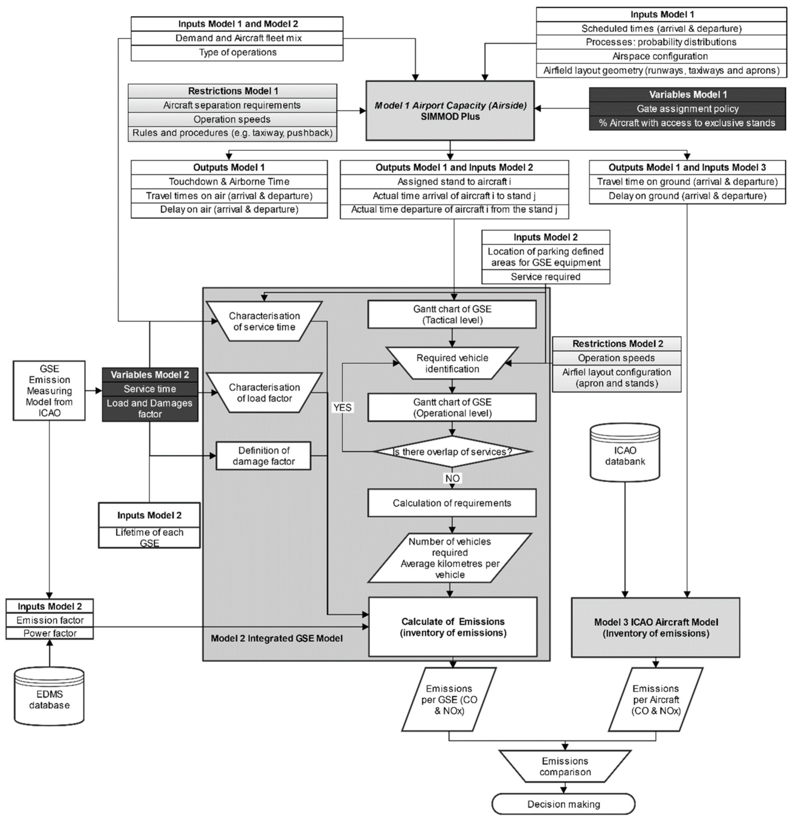
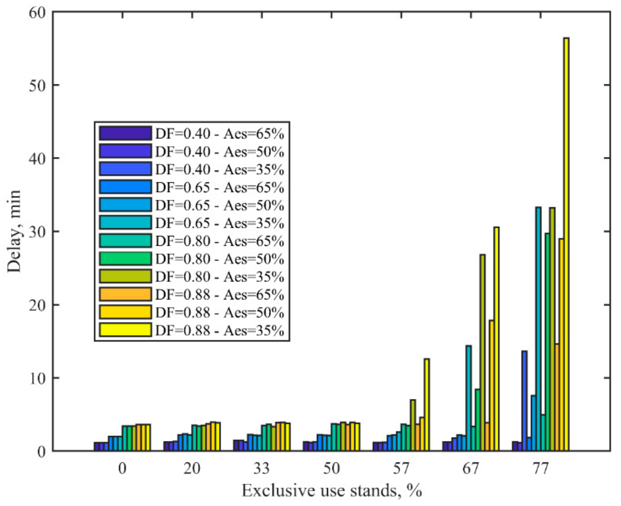
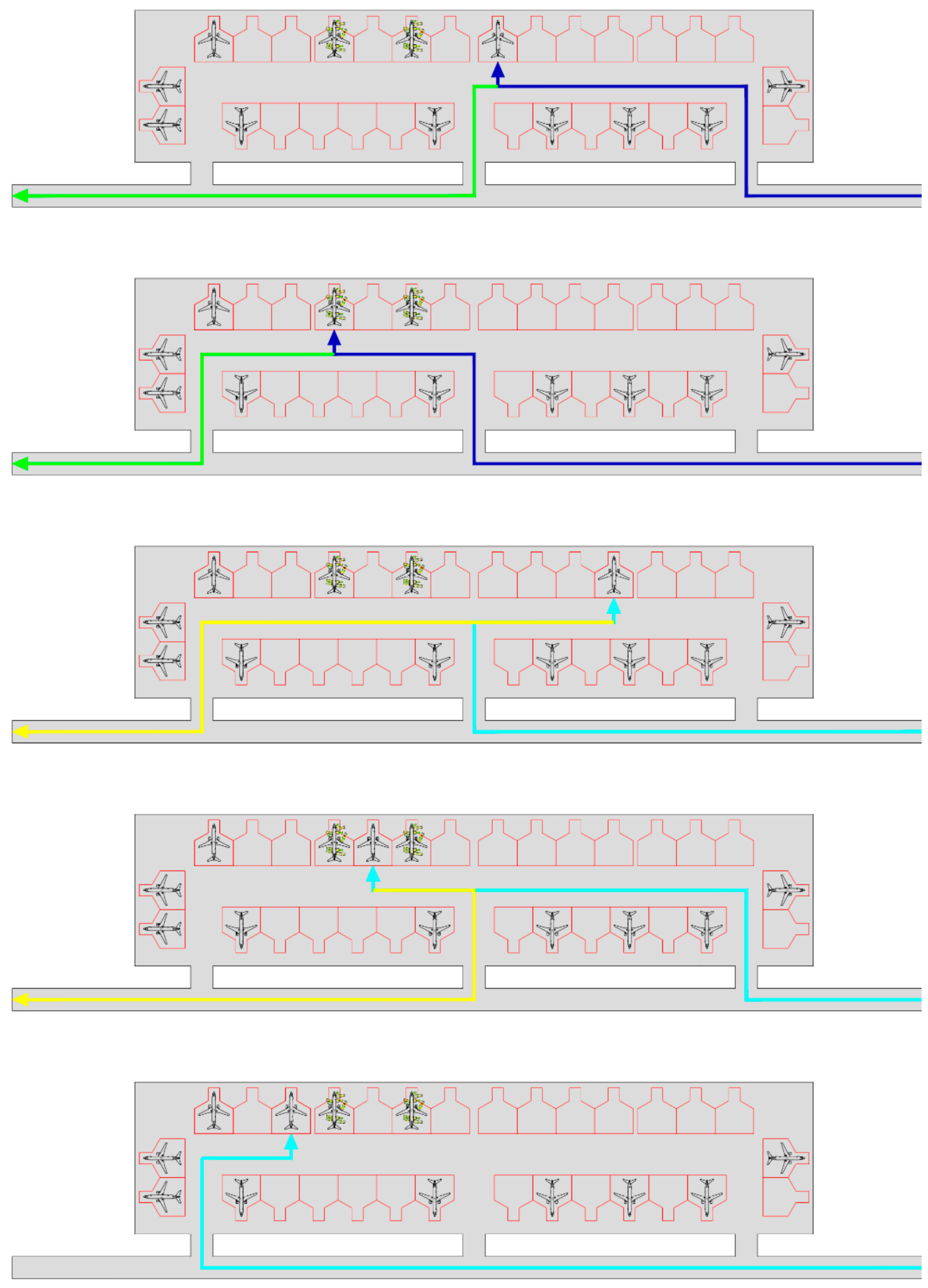
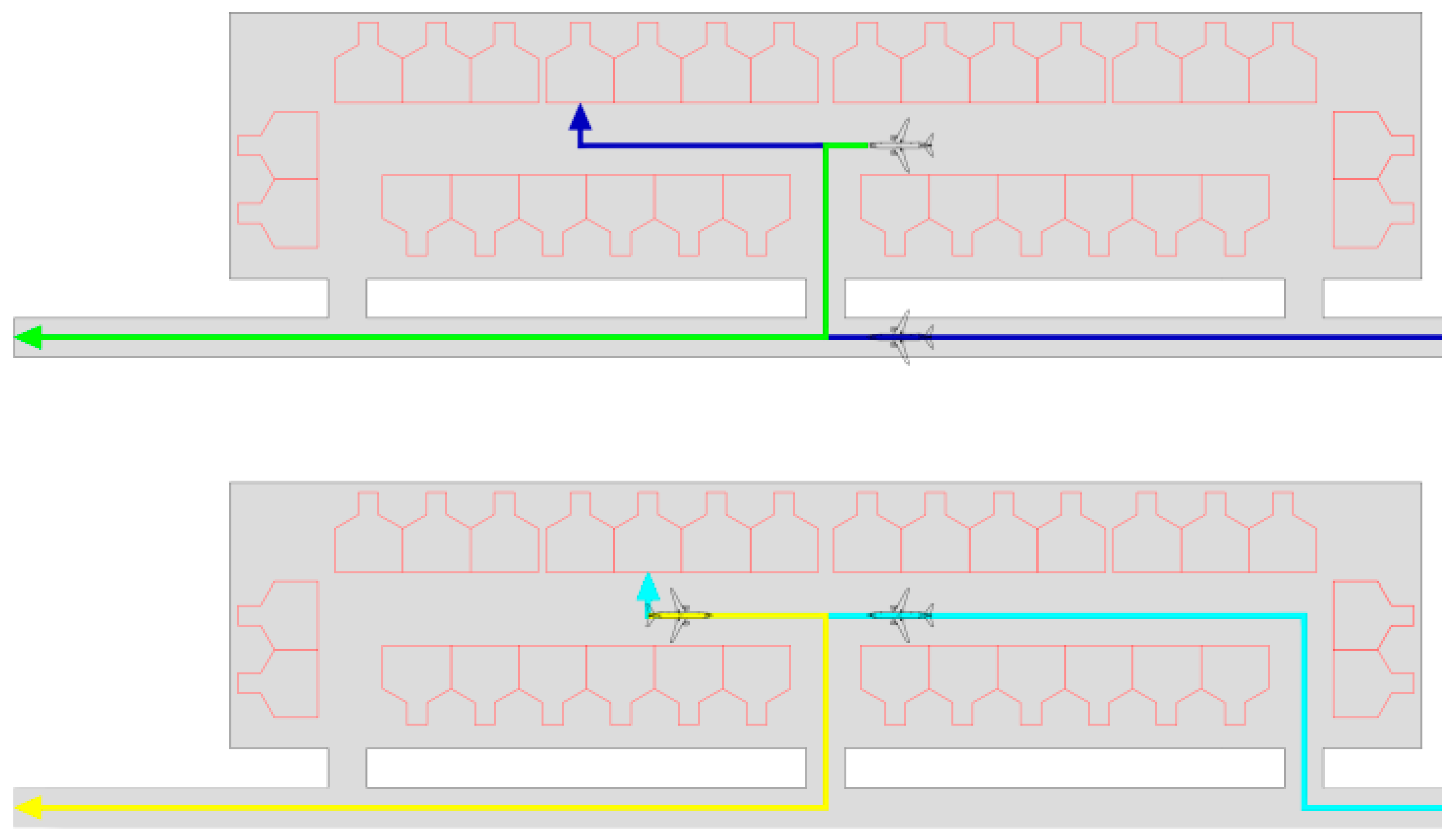
- In the first stage, SIMMOD Plus tool (called Model 1) is used to simulate operations of aircraft on the ground, particularly on the apron. SIMMOD software is a simulation program of discreet events which allows us to study the flight field dynamic, airspace routes, taxiing operations, and departure queues sequences, among other events related to the system capacity and the delay associated with it. The software allows us to quantify the delay based on the conditional operational rules included in the model, which specify the actions to be carried out by the simulation based on the system state.
- In this study, delay is measured in minutes and defined as “the time necessary to meet the requirements of a second aircraft when, at the same time, two aircraft request the same service”.
- The second stage corresponds to the implementation of Model 2, aiming at the study and quantification of GSE emissions produced by apron circulation and service. To do this, the covered distances are estimated through the assignment of gates. Aircraft service stage times are discretized, and other factors associated with GSE operations are identified, such as power, loading, damages, and emission factors.
3.3.1. Assumptions
- Distance between aircraft on the ground: 100 m
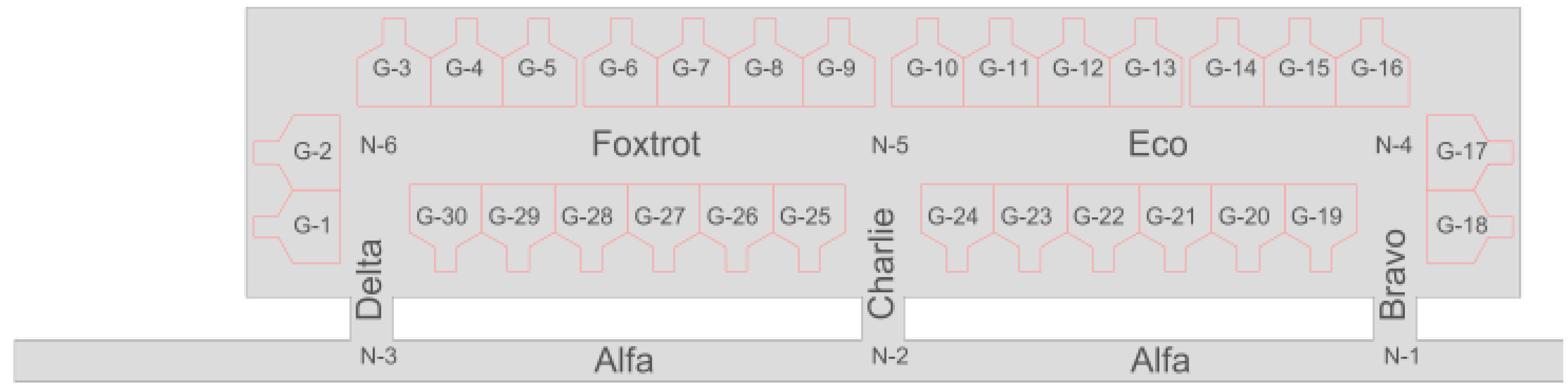
- Taxiing speed in parallel taxiway (Alfa): 20 km/h
- Taxiing speed in apron taxiway (Bravo, Charlie, Delta, Eco, Foxtrot): 10 km/h
- Stand access speed: 5 km/h
- Pushback speed: 4 km/h
- Unique handling service provider
- Same manufacturing year for every unit of each GSE
- Equal type of fuel: diesel for each GSE
- Operation speed on ramp of 20 km/h
3.3.2. Basic Structure
Model 1—Simulation Tool
Model 2—Integrated GSE Model
Model 3—Aircraft Emission
4. Results
4.1. Description of Inputs
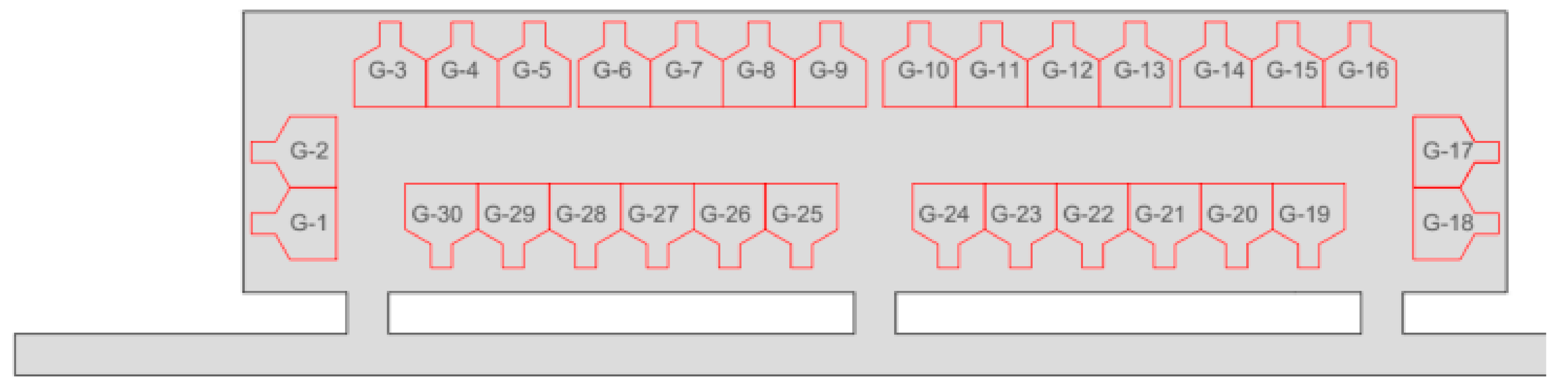
- Type A procedure: According to the equipment availability, a transfer between temporal GSE parking stands (ESA) can be simulated depending on the number of aircraft stands (Type C as they are defined on the apron configuration) that they have to go through for the next service.
- Type B procedure: These vehicles always have to return to a particular operation area after providing the service to the aircraft. Therefore, it is easy to measure the transfer distance because the team goes to every aircraft parking stand and returns to its determined fixed area before moving to another aircraft.
- Type C procedure: Since this equipment has a fixed parking stand, transfer distances can be estimated depending on the first arrival, along with service sequence for three extra aircraft according to the loading capacity before going back to their fixed parking stand to restock or unload wastes.
4.2. Analysis of Results
5. Conclusions
Author Contributions
Funding
Institutional Review Board Statement
Informed Consent Statement
Data Availability Statement
Acknowledgments
Conflicts of Interest
Nomenclature
| Aes | Aircraft with priority |
| Distance shipped for GSE ‘l’, . | |
| DF | Demand Factor |
| Contaminant emissions ‘i’, in regard to GSE ‘l’. | |
| Emission factor of pollutant ‘i’, in regard to GSE ‘l’, . | |
| Load factor for GSE ‘l, dimensionless. | |
| Damage factor for GSE ‘l’, dimensionless. | |
| GSE | Ground Support equipment |
| LC | Low-Cost carrier flight |
| LTO | Landing Take off cycle |
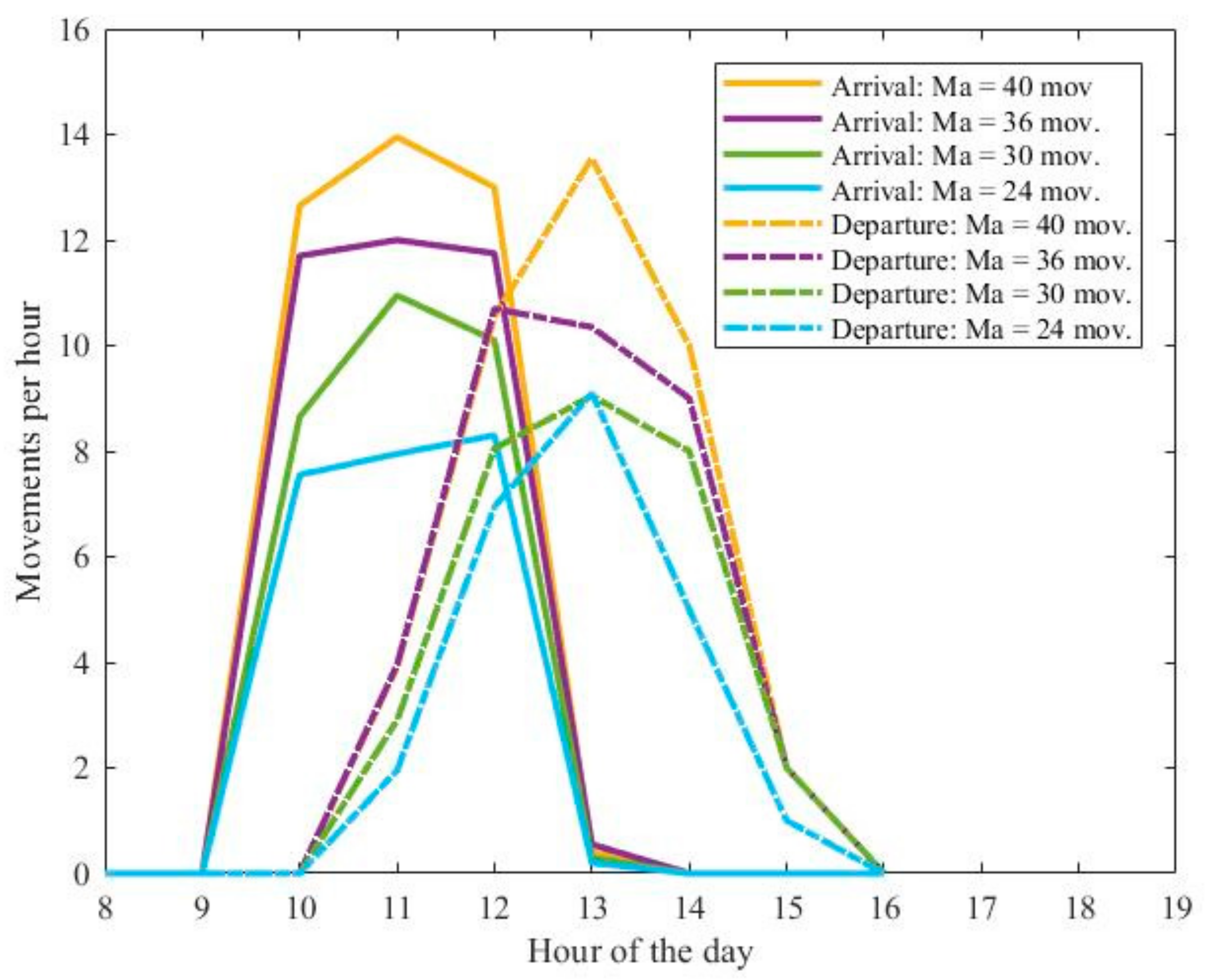
| Ma | Total arrival movements |
| Se | Exclusive use stands |
| St | Total parking stands |
| Ta | Arrival time frame |
| Pi | Break power for GSE ‘l’, |
| Sce | scenario: |
| V | Velocity of circulation for GSE ‘l’, |
| GSE discretization on waiting, connection, service and disconnection for load and unload . | |
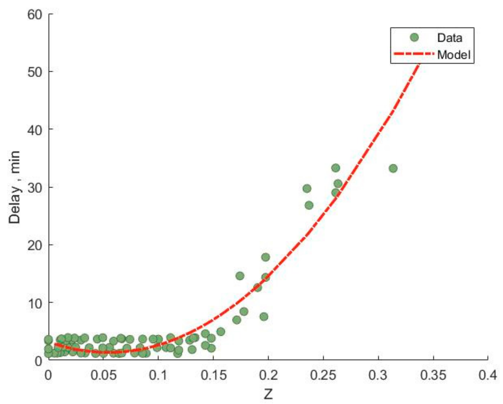
| Z | is a variable built according to the analysis of data and variables using R Studio software. |
Appendix A. Conflict Resolution Rules


Appendix B. Characterization of Processes—Probability Distributions


Appendix C. GSE Factor

| Code GSE | GSE | Power [HP] | Load Factor |
|---|---|---|---|
| BT | Baggage tractor | 88 | 0.475 |
| BL | Belt loader | 88 | 0.350 |
| TUG | TUG | 134 | 0.375 |
| BUS | Bus | 177 | 0.363 |
| R. BUS | Bus for passengers with reduced mobility | 330 | 0.283 |
| CAT | Catering | 330 | 0.490 |
| LV | Vacuum toilet | 75 | 0.283 |
| WP | Water potable | 235 | 0.263 |
| CLE | Cleaning | - | 0.350 |
| GPU | Ground Power Unit | 187 | 0.475 |
| PS | Passenger stairs | 88 | 0.475 |
| FUEL | Fuel truck | 320 | 0.388 |
| GSE | Load Factors | |||
|---|---|---|---|---|
| Waiting | Connection | Service | Disconnection | |
| Baggage tractor | 0.36 | 0.36 | 0.55 | 0.36 |
| Belt loader | 0.36 | 0.36 | 0 | 0.36 |
| TUG | 0.40 | 0.40 | 0.80 | 0.40 |
| Bus | 0.20 | 0 | 0.20 | 0 |
| R. Bus | 0.20 | 0 | 0.20 | 0 |
| Catering | 0.53 | 0.53 | 0 | 0.53 |
| Lavatory | 0.25 | 0.25 | 0.25 | 0.25 |
| Water potable | 0.20 | 0.20 | 0.20 | 0.20 |
| Cleaning | 0.33 | 0 | 0 | 0 |
| Ground Power Unit | 0 | 0 | 0.8 | 0 |
| Passenger stairs | 0.57 | 0 | 0 | 0 |
| Fuel truck | 0 | 0.25 | 1 | 0.25 |
| GSE | Load Factors | |||
|---|---|---|---|---|
| Waiting | Connection | Service | Disconnection | |
| Baggage tractor | 0.36 | 0.36 | 0.55 | 0.36 |
| Belt loader | 0.36 | 0.36 | 0 | 0.36 |
| TUG | 0 | 0 | 0 | 0 |
| Bus | 0.20 | 0 | 0.20 | 0 |
| R. Bus | 0.20 | 0 | 0.20 | 0 |
| Catering | 0.53 | 0.53 | 0 | 0.53 |
| Lavatory | 0.25 | 0.25 | 0 | 0.25 |
| Water potable | 0.20 | 0.20 | 0 | 0.20 |
| Cleaning | 0.33 | 0 | 0 | 0 |
| Ground Power Unit | 0 | 0 | 0 | 0 |
| Passenger stairs | 0.57 | 0 | 0 | 0 |
| Fuel truck | 0 | 0.25 | 1 | 0.25 |
| GSE | CO ‘i’ | NOx ‘i’ |
|---|---|---|
| (g/HP.h) | (g/HP.h) | |
| Baggage tractor | 1.503 | 4.485 |
| Belt loader | 2.553 | 4.544 |
| TUG | 1.503 | 4.485 |
| Bus | 0.110 | 2.500 |
| Catering | 0.449 | 1.037 |
| Vacuum toilet | 0.654 | 2.417 |
| Water potable | 0.804 | 2.898 |
| Ground Power Unit | 0.961 | 4.135 |
| Passenger stairs | 0.801 | 2.891 |
| Fuel truck | 0.614 | 2.184 |
| GSE | Use (Years) | Lifespan (Years) | CO | NOx |
|---|---|---|---|---|
| Baggage tractor | 8 | 13 | 1.092 | 1.005 |
| Belt loader | 8 | 11 | 1.092 | 1.005 |
| TUG | 8 | 14 | 1.086 | 1.005 |
| Bus | 8 | 10 | 1.100 | 1.005 |
| R. Bus | 8 | 10 | 1.100 | 1.006 |
| Catering | 8 | 10 | 1120 | 1.006 |
| Vacuum toilet | 8 | 13 | 1.120 | 1.006 |
| Water potable | 8 | 10 | 1.120 | 1.006 |
| Ground Power Unit | 8 | 14 | 1.120 | 1.006 |
| Passenger stairs | 8 | 14 | 1.120 | 1.006 |
| Fuel truck | 8 | 14 | 1.086 | 1.005 |
References
- Wing, A.K.; Felder, W.N.; Cloutier, R.J. Modeling a Ramp Area Support System. In Proceedings of the 15th AIAA Aviation Technology, Integration, and Operations Conference, Dallas, TX, USA, 22–26 June 2015; American Institute of Aeronautics and Astronautics: Reston, VA, USA, 2015. [Google Scholar] [CrossRef]
- Schmidt, M.; Paul, A.; Cole, M.; Ploetner, K.O. Challenges for ground operations arising from aircraft concepts using alternative energy. J. Air Transp. Manag. 2016, 56, 107–117. [Google Scholar] [CrossRef]
- Palocz-Andresen, M. Emissions at airports and their impact at the habitat. Period. Polytech. Mech. Eng. 2009, 53, 13. [Google Scholar] [CrossRef]
- Hannah, J.; Hettmann, D.; Rashid, N.; Saleh, C.; Yilmaz, C. Design of a carbon neutral airport. In Proceedings of the 2012 IEEE Systems and Information Engineering Design Symposium, Institute of Electrical and Electronics Engineers (IEEE), Charlottesville, VA, USA, 27–27 April 2012; pp. 40–45. [Google Scholar] [CrossRef]
- Winther, M.; Kousgaard, U.; Ellermann, T.; Massling, A.; Nøjgaard, J.K.; Ketzel, M. Emissions of NOx, particle mass and particle numbers from aircraft main engines, APU’s and handling equipment at Copenhagen Airport. Atmos. Environ. 2015, 100, 218–299. [Google Scholar] [CrossRef]
- Airport Air Quality Manual Doc 9889; International Civil Aviation Organization (ICAO): Montreal, QC, Canada, 2011; Volume 1.
- Mirkovic, B.; Tošić, V. Airport apron capacity: Estimation, representation, and flexibility. J. Adv. Transp. 2013, 48, 97–118. [Google Scholar] [CrossRef]
- Mirković, B.; Tošić, V. The difference between hub and non-hub airports—An airside capacity perspective. J. Air Transp. Manag. 2017, 62, 121–128. [Google Scholar] [CrossRef]
- Deng, W.; Sun, M.; Zhao, H.; Li, B.; Wang, C. Study on an airport gate assignment method based on improved ACO algorithm. Kybernetes 2018, 47, 20–43. [Google Scholar] [CrossRef]
- Guclu, O.E.; Cetek, C. Analysis of aircraft ground traffic flow and gate utilisation using a hybrid dynamic gate and taxiway assignment algorithm. Aeronaut. J. 2017, 121, 721–745. [Google Scholar] [CrossRef]
- Kim, S.H.; Feron, E.; Clarke, J.-P. Assigning gates by resolving physical conflicts. In Proceedings of the AIAA Guidance, Navigation, and Control Conference, Chicago, IL, USA, 10–13 August 2009; p. 16. [Google Scholar] [CrossRef]
- Carpenter, M.; Stroiney, S. Managing gate and ramp operations to reduce delay, fuel burn, and costs. In Proceedings of the 2012 Integrated Communications, Navigation and Surveillance Conference, Herndon, VA, USA, 24–26 April 2012. [Google Scholar] [CrossRef]
- Kuzu, S.L. Estimation and dispersion modeling of landing and take-off (LTO) cycle emissions from Atatürk International Airport. Air Qual. Atmos. Health 2017, 11, 153–161. [Google Scholar] [CrossRef]
- Janić, M. Analyzing, modeling, and assessing the performances of land use by airports. Int. J. Sustain. Transp. 2015, 10, 683–702. [Google Scholar] [CrossRef] [Green Version]
- Mota, M.M.; Boosten, G.; De Bock, N.; Jimenez, E.; de Sousa, J.P. Simulation-based turnaround evaluation for Lelystad Airport. J. Air Transp. Manag. 2017, 64, 21–32. [Google Scholar] [CrossRef]
- Mota, M.; Di Bernardi, A.; Scala, P.; Ramirez-diaz, G. Simulation-based virtual cycle for multi-level airport analysis. Aerosp. Sci. Technol. 2018, 5, 44. [Google Scholar] [CrossRef] [Green Version]
- Ferrulli, P. Green airport design evaluation (GrADE)—Methods and tools improving infrastructure planning. Transp. Res. Procedia 2016, 14, 3781–3790. [Google Scholar] [CrossRef] [Green Version]
- Challenges of Growth 2013—Task 4: European Air Traffic in 2035; Eurocontrol: Brussels, Belgium, 2013.
- Yılmaz, I. Emissions from passenger aircraft at Kayseri Airport, Turkey. J. Air Transp. Manag. 2017, 58, 176–182. [Google Scholar] [CrossRef]
- Edb-Emissions-Databank v25a (web); International Civil Aviation Organization (ICAO): Montreal, QC, Canada, 2018.
- Tan, Y.L. Differences in Ground Handling in the Global Market Yik Lun Tan; Project of Hamburg University of Applied Sciences: Hambourg, Germany, 2010; pp. 1–34. [Google Scholar]
- Fleuti, E. Aircraft Ground Handling Emissions; Zurich Airport: Flughafen Zürich, Switzerland, 2014; p. 20. [Google Scholar]
- Wu, C.; Caves, R.E. Modelling and optimization of aircraft turnaround time at an airport. Transp. Plan. Technol. 2004, 27, 47–66. [Google Scholar] [CrossRef]
- Coupe, J.; Milutinovic, D.; Malik, W.; Jung, Y.C. A Data Driven Approach for Characterization of Ramp Area Push Back and Ramp-Taxi Processes. In Proceedings of the 16th AIAA Aviation Technology, Integration, and Operations Conference, Washington, DC, USA, 13–17 June 2016; pp. 1–15. [Google Scholar] [CrossRef] [Green Version]


| Variables | Values |
|---|---|
| DF | 0.40, 0.65, 0.80, 0.88 |
| %Se | 0, 6/30, 10/30, 15/30, 17/30, 20/30, 23/30 |
| %Aes | 35%, 50%, 65% |
| Code GSE | GSE ‘l’ | Waiting | Connection | Service | Disconnection | Total |
|---|---|---|---|---|---|---|
| BT | Baggage tractor | 92 | 20 | 531 | 13 | 547 |
| BL | Belt loader | 105 | 38 | 924 | 124 | 1191 |
| TUG | Tug | 30 | 131 | 315 | 24 | 501 |
| BUS | Bus | 53 | 0 | 292 | 0 | 332 |
| R. BUS | R. Bus | 51 | 110 | 476 | 98 | 735 |
| CAT | Catering | 134 | 102 | 376 | 109 | 721 |
| LV | Vacuum toilet | - | - | - | - | - |
| WP | Water potable | 24 | 18 | 48 | 34 | 124 |
| CLE | Cleaning | 58 | 0 | 640 | 0 | 698 |
| GPU | Ground Power Unit | 0 | 259 | 4386 | 21 | 4666 |
| PS | Passenger stairs | 68 | 54 | 298 | 0 | 419 |
| FUEL | Fuel truck | 930 | 63 | 531 | 143 | 1667 |
| Type of Procedure | GSE Model | GSE Parking Stand |
|---|---|---|
| A | Conveyor Freight elevators Aircraft towing GPU tractor Passenger stair | Each equipment staging area (ESA) according to service time per aircraft [1]. |
| B | Baggage tractor Transp. PAX with reduced mobility Passenger transport | Fixed parking area where passengers are taken after the aircraft arrival [2]. |
| C | Catering truck Waste water cleaning Water supply Fuel tanker | Catering, cleaning, and water supplying vehicles are parked outside the apron [3]. The tanker has assigned parking stands in the fuel plant on the airport grounds. |
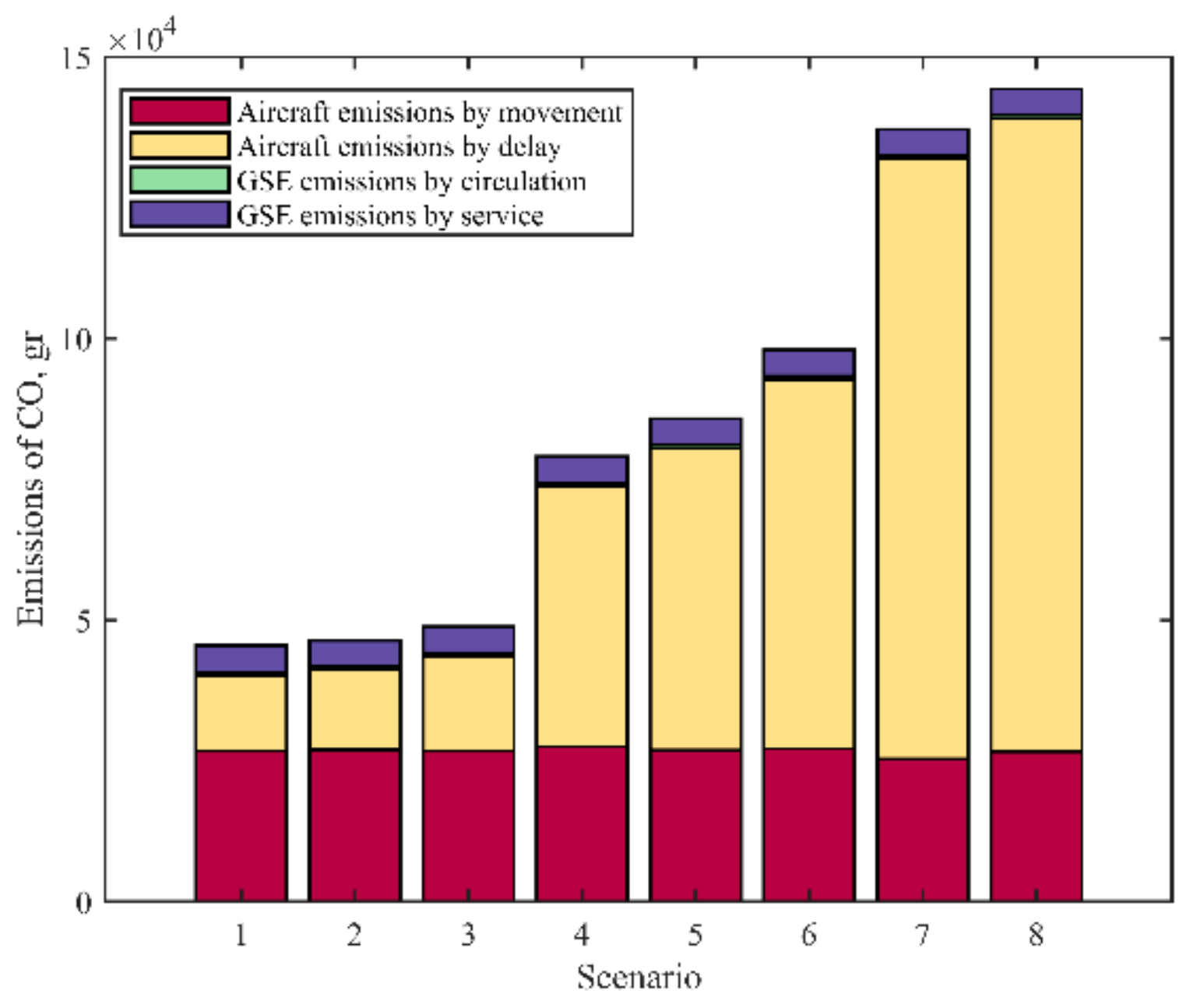
| Scenario | %Aes | %Se |
|---|---|---|
| 1 | 67 | 57 |
| 2 | 67 | 67 |
| 3 | 50 | 57 |
| 4 | 33 | 57 |
| 5 | 67 | 77 |
| 6 | 50 | 67 |
| 7 | 50 | 77 |
| 8 | 33 | 67 |
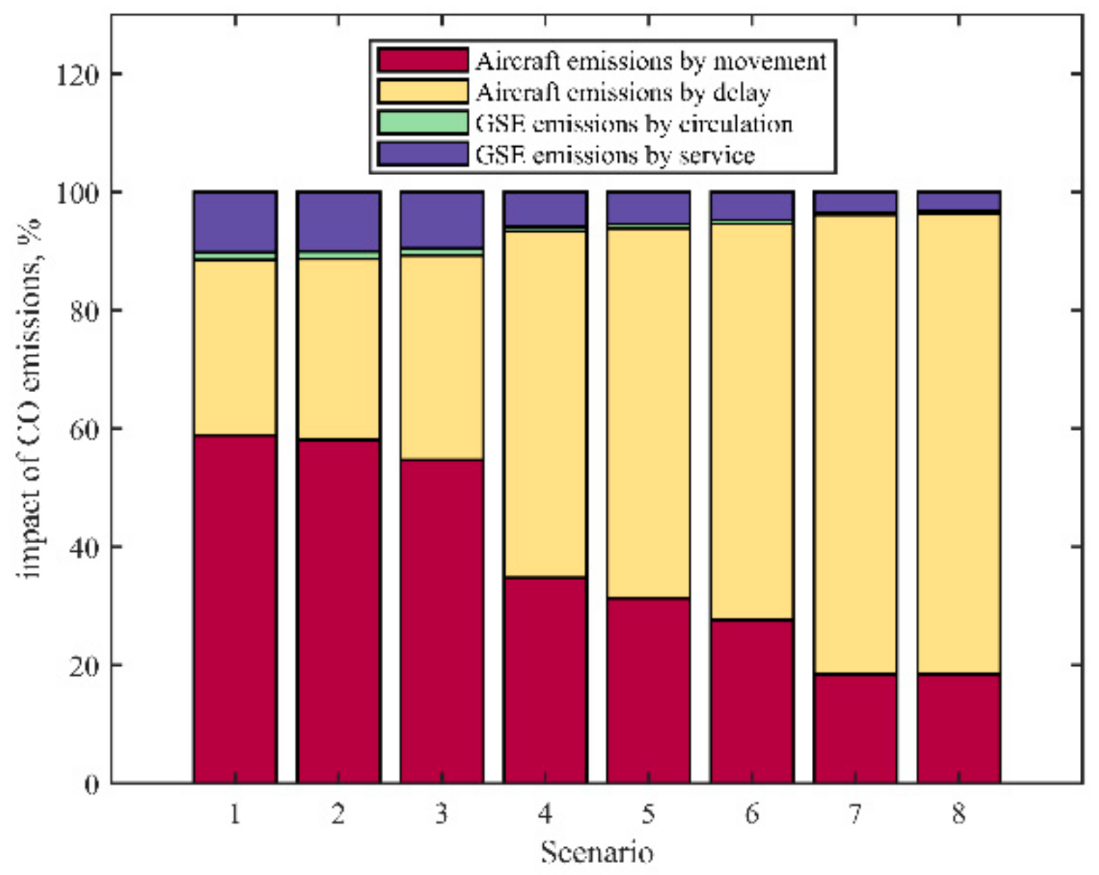
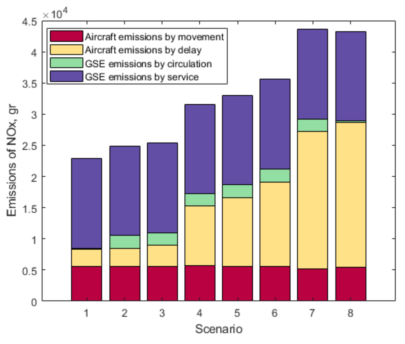
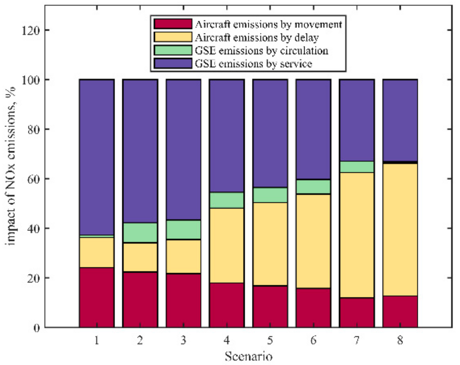
| Scenario | 1 | 2 | 3 | 4 | 5 | 6 | 7 | 8 |
|---|---|---|---|---|---|---|---|---|
| CO, Travel aircraft | 58.87 | 58.16 | 54.74 | 34.82 | 31.31 | 27.71 | 18.45 | 18.48 |
| CO, Delay aircraft | 29.62 | 30.53 | 34.55 | 58.54 | 62.58 | 66.93 | 77.73 | 77.90 |
| CO, GSE per circulation | 1.29 | 1.29 | 1.21 | 0.76 | 0.70 | 0.62 | 0.44 | 0.40 |
| CO, GSE per service | 10.22 | 10.02 | 9.51 | 5.88 | 5.41 | 4.74 | 3.39 | 3.22 |
| NOx, Travel aircraft | 5.519 | 5.565 | 5.519 | 5.678 | 5.542 | 5.602 | 5.223 | 5.504 |
| NOx, Delay aircraft | 2.777 | 2.921 | 3.483 | 9.546 | 11.078 | 13.529 | 22.005 | 23.197 |
| NOx, GSE per circulation | 230 | 2.015 | 2.003 | 2.030 | 2.022 | 2.097 | 2.011 | 235 |
| NOx, GSE per service | 14.335 | 14.335 | 14.335 | 14.335 | 14.335 | 14.335 | 14.335 | 14.335 |
| Scenarios | ||||||||
|---|---|---|---|---|---|---|---|---|
| GSE | 1 | 2 | 3 | 4 | 5 | 6 | 7 | 8 |
| BT | 12 | 10 | 10 | 12 | 12 | 10 | 10 | 10 |
| BL | 10 | 8 | 10 | 10 | 10 | 10 | 10 | 10 |
| Bus | 10 | 8 | 10 | 12 | 10 | 10 | 14 | 10 |
| PS | 8 | 8 | 10 | 10 | 8 | 10 | 10 | 10 |
| CAT | 7 | 7 | 7 | 7 | 7 | 7 | 8 | 7 |
| LV | 5 | 5 | 5 | 5 | 5 | 5 | 5 | 5 |
| WP | 4 | 4 | 4 | 4 | 5 | 5 | 4 | 4 |
| GPU | 4 | 5 | 5 | 5 | 4 | 4 | 4 | 3 |
| Tug | 2 | 2 | 2 | 2 | 2 | 2 | 3 | 3 |
| GSE | 1 | 2 | 3 | 4 | 5 | 6 | 7 | 8 |
|---|---|---|---|---|---|---|---|---|
| BT | 12.52 | 14.48 | 19.12 | 15.80 | 13.66 | 19.12 | 15.36 | 20.82 |
| BL | 11.47 | 11.58 | 8.69 | 11.74 | 13.51 | 11.86 | 12.26 | 10.49 |
| Bus | 9.64 | 13.28 | 11.68 | 15.34 | 15.62 | 18.46 | 13.09 | 20.48 |
| PS | 7.31 | 8.43 | 8.33 | 6.07 | 5.78 | 11.35 | 7.74 | 8.07 |
| CAT | 12.69 | 13.94 | 13.33 | 14.36 | 13.53 | 13.47 | 15.85 | 14.63 |
| LV | 12.43 | 11.98 | 11.82 | 11.93 | 11.31 | 12.22 | 10.90 | 12.40 |
| WP | 9.76 | 10.96 | 10.94 | 9.99 | 12.01 | 10.79 | 11.86 | 12.29 |
| GPU | 7.58 | 5.93 | 6.51 | 5.49 | 6.13 | 6.53 | 6.49 | 5.18 |
| Tug | 3.27 | 3.43 | 4.05 | 3.62 | 2.63 | 2.59 | 3.20 | 2.70 |
| GSE | 1 | 2 | 3 | 4 | 5 | 6 | 7 | 8 |
|---|---|---|---|---|---|---|---|---|
| BT | 1.04 | 1.45 | 1.91 | 1.32 | 1.14 | 1.91 | 1.54 | 2.08 |
| BL | 1.15 | 1.45 | 0.87 | 1.17 | 1.35 | 1.19 | 1.23 | 1.05 |
| Bus | 0.96 | 1.66 | 1.17 | 1.28 | 1.56 | 1.85 | 0.93 | 2.05 |
| PS | 0.91 | 1.05 | 0.83 | 0.61 | 0.72 | 1.14 | 0.77 | 0.81 |
| CAT | 1.81 | 1.99 | 1.90 | 2.05 | 1.93 | 1.92 | 1.98 | 2.09 |
| LV | 2.49 | 2.40 | 2.36 | 2.39 | 2.26 | 2.44 | 2.18 | 2.48 |
| WP | 2.44 | 2.74 | 2.73 | 2.50 | 2.40 | 2.16 | 2.96 | 3.07 |
| GPU | 1.89 | 1.19 | 1.30 | 1.10 | 1.53 | 1.63 | 1.62 | 1.73 |
| Tug | 1.64 | 1.71 | 2.02 | 1.81 | 1.32 | 1.30 | 1.07 | 0.90 |
| Scenario | Number of Vehicles Required | Average Kilometers per Vehicle |
|---|---|---|
| 1 | 10 | 9.3 |
| 2 | 11 | 8.5 |
| 3 | 11 | 8.4 |
| 4 | 12 | 7.8 |
| 5 | 10 | 9.3 |
| 6 | 12 | 7.7 |
| 7 | 10 | 9.1 |
| 8 | 10 | 8.6 |
Publisher’s Note: MDPI stays neutral with regard to jurisdictional claims in published maps and institutional affiliations. |
© 2021 by the authors. Licensee MDPI, Basel, Switzerland. This article is an open access article distributed under the terms and conditions of the Creative Commons Attribution (CC BY) license (http://creativecommons.org/licenses/by/4.0/).
Share and Cite
Sznajderman, L.; Ramírez-Díaz, G.; Di Bernardi, C.A. Influence of the Apron Parking Stand Management Policy on Aircraft and Ground Support Equipment (GSE) Gaseous Emissions at Airports. Aerospace 2021, 8, 87. https://doi.org/10.3390/aerospace8030087
Sznajderman L, Ramírez-Díaz G, Di Bernardi CA. Influence of the Apron Parking Stand Management Policy on Aircraft and Ground Support Equipment (GSE) Gaseous Emissions at Airports. Aerospace. 2021; 8(3):87. https://doi.org/10.3390/aerospace8030087
Chicago/Turabian StyleSznajderman, Lucas, Gabriel Ramírez-Díaz, and Carlos A. Di Bernardi. 2021. "Influence of the Apron Parking Stand Management Policy on Aircraft and Ground Support Equipment (GSE) Gaseous Emissions at Airports" Aerospace 8, no. 3: 87. https://doi.org/10.3390/aerospace8030087