Article

Sensitivity Study of Ice Accretion Simulation to Roughness Thermal Correction Model

by
Kevin Ignatowicz
1,*,
François Morency
1 and
Héloïse Beaugendre
2
1
École de Technologie Supérieure, Mechanical Engineering Department, Montreal, QC H3C1K3, Canada
2
University of Bordeaux, INRIA, CNRS, Bordeaux INP, IMB, UMR 5251, F-33400 Talence, France
*
Author to whom correspondence should be addressed.
Aerospace 2021, 8(3), 84; https://doi.org/10.3390/aerospace8030084
Submission received: 6 December 2020 / Revised: 5 March 2021 / Accepted: 17 March 2021 / Published: 19 March 2021

Abstract

:
The effects of atmospheric icing can be anticipated by Computational Fluid Dynamics (CFD). Past studies show that the convective heat transfer influences the ice accretion and is itself a function of surface roughness. Uncertainty quantification (UQ) could help quantify the impact of surface roughness parameters on the reliability of ice accretion prediction. This paper aims to quantify ice accretion uncertainties and identify the key surface roughness correction parameters contributing the most to the uncertainties in a Reynolds-Averaged Navier-Stokes (RANS) formulation. Ice accretion simulations over a rough flat plate using two thermal correction models are used to construct a RANS database. Non-Intrusive Polynomial Chaos Expansion (NIPCE) metamodels are developed to predict the convective heat transfer and icing characteristics of the RANS database. The metamodels allow for the computation of the 95% confidence intervals of the output probability distribution (PDF) and of the sensitivity indexes of the roughness parameters according to their level of influence on the outputs. For one of the thermal correction models, the most influential parameter is the roughness height, whereas for the second model it is the surface correction coefficient. In addition, the uncertainty on the freestream temperature has a minor impact on the ice accretion sensitivity compared to the uncertainty on the roughness parameters.

1. Introduction

Icing represents a major threat to in-flight safety. Ice accretion leads to increased aircraft weight, aerodynamic efficiency loss and a potential increase of up to more than 60% in drag [1]. In the 1997–2006 period, 13% of weather-related accidents were caused by icing [2]. The aerodynamic efficiency loss is determined by the geometry of the ice shape, mainly the thickness and extension [3]. Developments in numerical simulations, especially RANS-based simulations (Reynolds Averaged Navier-Stokes), have enabled the development of icing codes, useful for the effective anticipation of the icing process [4]. Even if icing codes share similar mathematical models and numerical methods, the predicted ice shapes can vary greatly for the same atmospheric conditions [5]. The discrepancies between shapes can be explained by various reasons, both mathematical and numerical, among them the discrepancy between the convective heat transfer models. The fraction of the shape discrepancy that could be attributed to the thermal modeling remains to be quantified.
Most of the icing codes used to predict the ice accretion shape are based on the Messinger model [6]. The model uses a mass and energy balance involving the convective heat transfer to compute the ice growth on the airplane surface [7]. Past studies have shown that the convective heat transfer, modeled by a convective heat transfer coefficient, has a major impact on the final shape of the ice accretion [8,9]. The convective heat transfer coefficient does play a key role in the geometry of the ice shape, which needs to be quantified.
The increase in surface roughness due to early ice formation has an impact on the convective heat transfer in the near-wall region. Experimental studies were conducted by NASA to measure the convective heat transfer coefficient, or, equivalently, the Stanton number, on a roughened NACA0012 airfoil [10,11]. More recently, by Liu & Hu [12], Hosni et al. [13] and Dukhan et al. [14,15] also carried out related experiments, but on a roughened flat plate, highlighting the influence of the roughness characteristics on the Stanton number. An increase in the heat transfer coefficient was observed for a rough surface as compared to a smooth one, in both airfoil and flat plate cases. From the foregoing, it is therefore reasonable to expect that the initial surface roughness of the wing is influencing the complete icing process by acting on the convective heat transfer at the surface [8,16]. Experimental studies show the variability of roughness characteristics, which depend mainly on the airfoil geometry [17] and atmospheric conditions [14]. The incorporation of surface roughness in the RANS model is then subject to uncertainty due to the prevailing lack of knowledge on roughness characteristics in real in-flight situations. The RANS model’s roughness parameters are thus epistemically uncertain variables.
To take into account the surface roughness, Aupoix [18] worked on improvements of the thermal boundary layer calculations by considering a local increment of the Prandtl number. The thermal correction model from Aupoix, denoted as the HAX model, uses three parameters to incorporate surface roughness in simulations: the roughness height, the equivalent sand grain roughness and the surface correction coefficient. Another thermal correction model, called the 2PP model, was developed and is also used in the present study [19]. This model relies on two parameters: the roughness height and the equivalent sand grain roughness. The parameters involved in both the HAX and 2PP models are denoted as the roughness parameters for the rest of the paper. To further improve these two models, sensibility studies can play a key role in establishing the most sensitive parameters. Once identified, it will be possible to vary these parameters in experiments or high-fidelity simulations in order to further calibrate and improve the thermal models.
For uncertain input parameters, the uncertainty quantification (UQ) enables the evaluation of the probability distribution function (PDF) of the output of interest and a complete sensitivity analysis [20]. A relatively small sample of RANS simulations is needed, and a metamodel is generated based on these sample results. This metamodel allows us to quickly compute a large number of new heat transfer coefficients and ice accretion results. The Non-Intrusive Polynomial Chaos Expansion (NIPCE) is commonly used for metamodel generation [21]. The NIPCE is an efficient approach to estimate measurement uncertainties when complex systems are involved, thus explaining its widespread use in UQ [22,23], especially in aeronautics applications [24]. The NIPCE approach is also used in turbulence modeling for UQ, as carried out in [25] to assess the Spalart-Allmaras uncertainty due to the epistemically uncertain model coefficients.
The sensitivity of an output parameter to the input parameter(s) can be evaluated by using a variance-based decomposition [26,27]. In the variance-based family, the Sobol indexes allow for an estimation of the main (first-order indexes) and interaction (second- and higher-order indexes) effects of an input parameter on the model output [28]. The Sobol indexes classify the input parameters according to their level of influence on a specific output parameter. UQ coupled to NIPCE and Sobol indexes has been used for simulations in aeronautics [29,30] and heat transfer [31]. Despite UQ’s wide use in aeronautics and heat transfer applications, no published paper has yet thoroughly characterized, from a statistical point of view, the sensitivity of ice accretion to surface roughness parameters. The closest related work is from Raj et al. [32], where the sensitivity of the ice accretions to the equivalent sand grain roughness is compared to the sensitivity to ice density, droplet distribution and number of ice layers. However, no comparison is made for the roughness parameters between them.
The present work is a first attempt to use UQ in aircraft icing to relate directly heat transfer model parameters to ice shape predictions. In addition, UQ allows the identification of the key parameters. The technical challenge in this case is double. First, an efficient way of generating a large sample set had to be used: making a sensitivity study requires a large database. The metamodel approach is well suited to this challenge, avoiding the computational effort that computational fluid dynamics (CFD) simulations would have required. Secondly, a reliable gauge of the importance of each roughness parameter was needed. The Sobol indexes give us the opportunity of directly reading on a bar chart the classification of the parameters depending on their level of influence on ice accretion. The objective is to quantify ice accretion uncertainty and identify the key roughness parameters contributing the most to the uncertainty of the thermal correction models for RANS equations. The importance of roughness parameters uncertainty compared to the freestream temperature uncertainty on the ice accretion shape is also investigated. To reduce the number of parameters, avoid curvature effects on ice growth and pressure gradients, the airfoil is replaced by a flat plate.
Metamodels generated from a sample of RANS simulations, alternatively using the HAX [18] and the 2PP [19] thermal correction models, are constructed to predict the convective heat transfer and ice accretions on a flat plate. For the ice accretion part, the flat plate has the droplet collection efficiency of a NACA0012, to be representative of an airfoil. The NIPCE metamodels are then used for UQ and to evaluate the Sobol sensitivity indexes associated with the roughness height, the equivalent sand grain roughness, the surface correction coefficient in the case of the HAX model and, finally, the freestream temperature. The novelty of the current work resides in the application of the NIPCE metamodeling method to rough icing simulations. The NIPCE has low sample requirements compared to the traditional Monte-Carlo methods used in the past [33]. In similar applications, Raj et al. [32] use the radial basis function (RBF) metamodeling. The performance of polynomial-type metamodels, like the NIPCE, compared to RBF methods, is better for small sample designs, giving higher regression coefficients [34]. This enhanced accuracy, which combined with the fast response due to the low sample sizes led to the choice of this tool to perform the metamodeling.
The paper starts with a presentation of the physical set-up where the flat plate geometry used is presented and contextualized, along with the HAX and 2PP RANS thermal correction models and the ice accretion model. Then, the methods retained for UQ and sensitivity analysis, including the NICPE metamodeling and the Sobol indexes, are described. Finally, the last section focuses on the results obtained from the simulations and the metamodeling process by highlighting the PDFs of the outputs and the Sobol indexes associated with the roughness parameters. The results allow for the determination of the most influential roughness parameter for both thermal correction models, and show the relative importance of roughness uncertainty compared to the freestream temperature uncertainty on the ice accretion shape.

2. Physical Set-Up

The goal of this section is, first, to define the test case geometrical configuration in the context of the RANS equations coupled to a Messinger model for ice accretion prediction. In this study, RANS equations are solved using a thermal correction model—either the HAX model or the 2PP model, which is presented in the second part of the section.

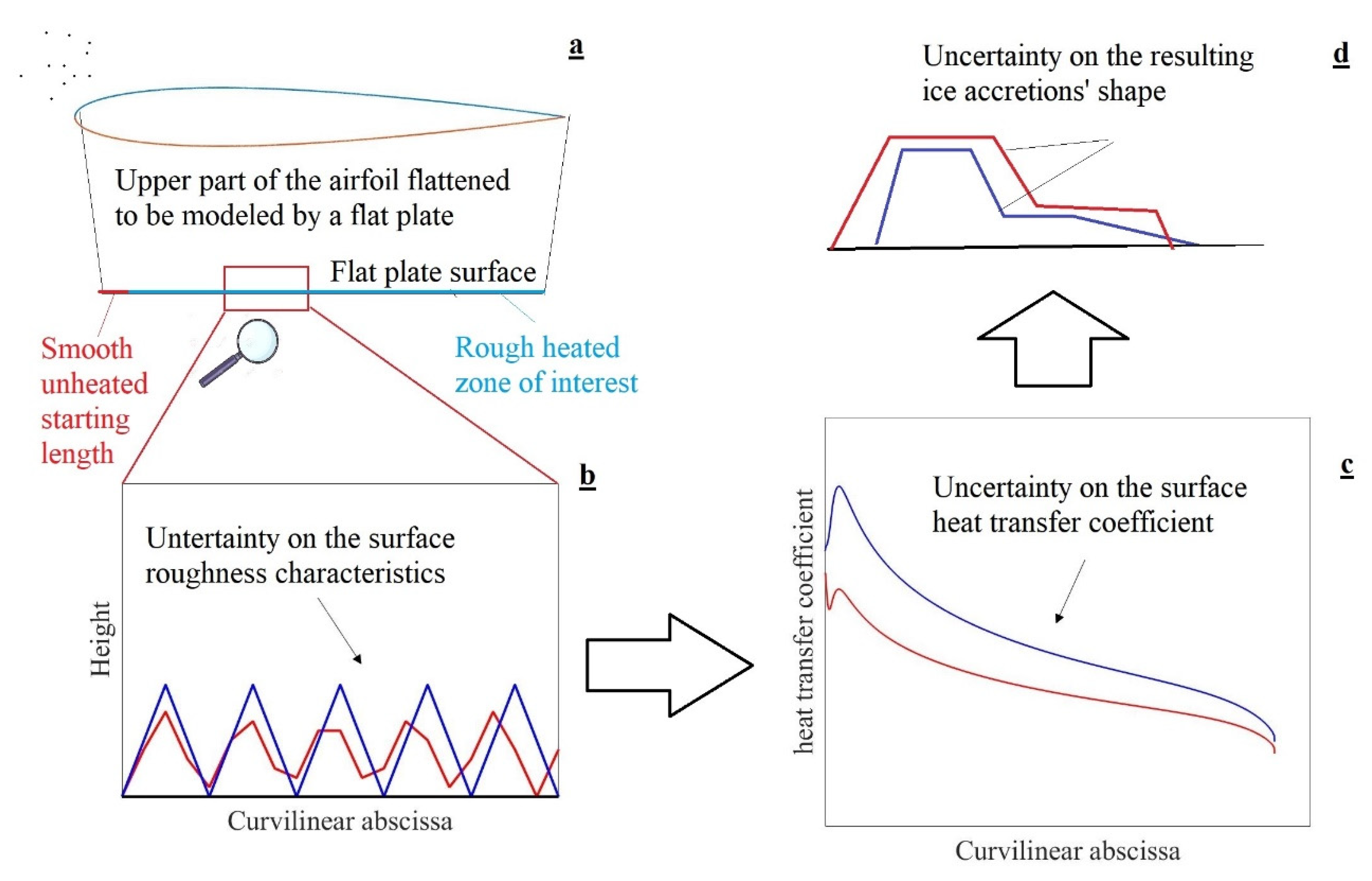
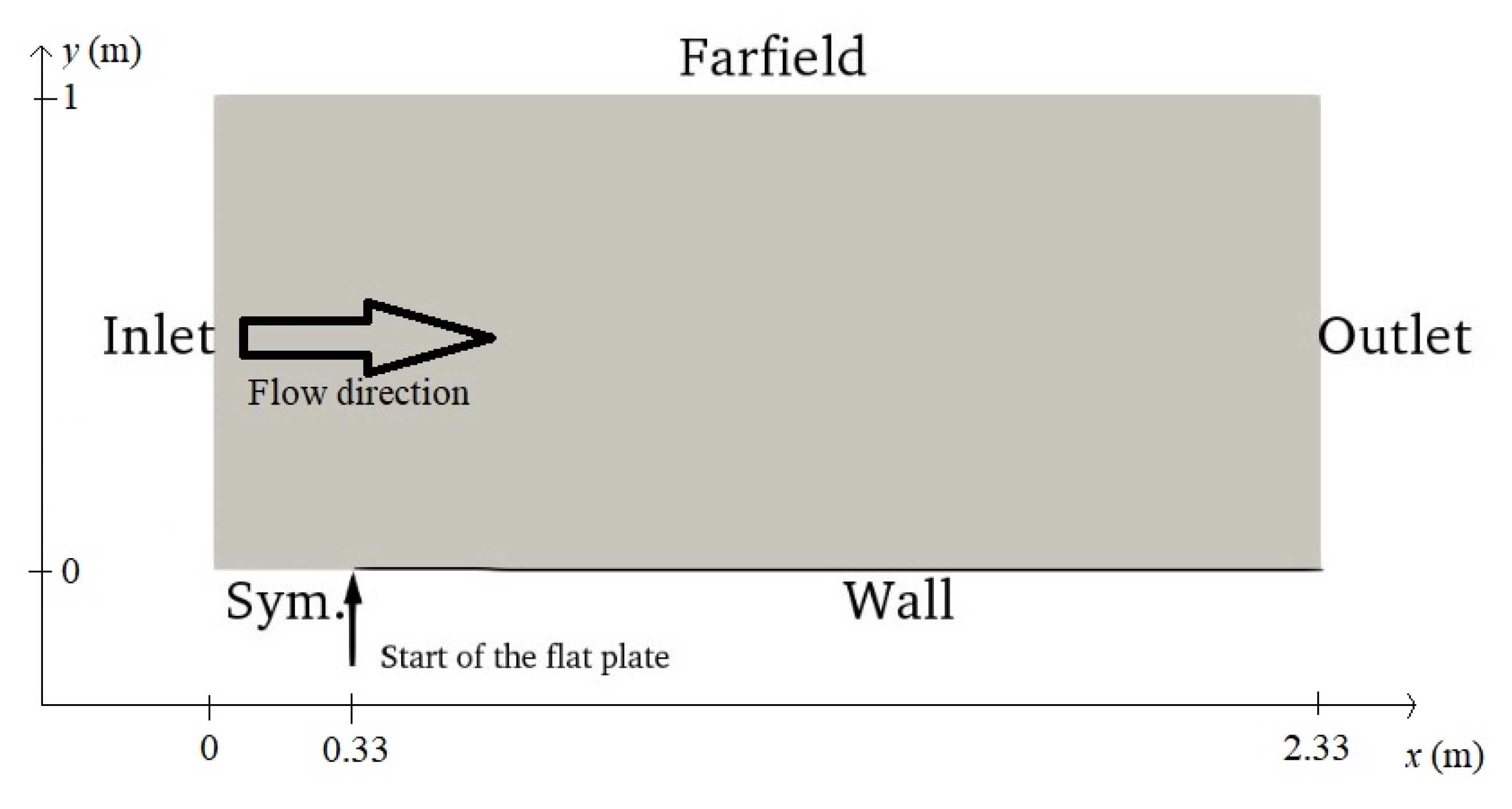
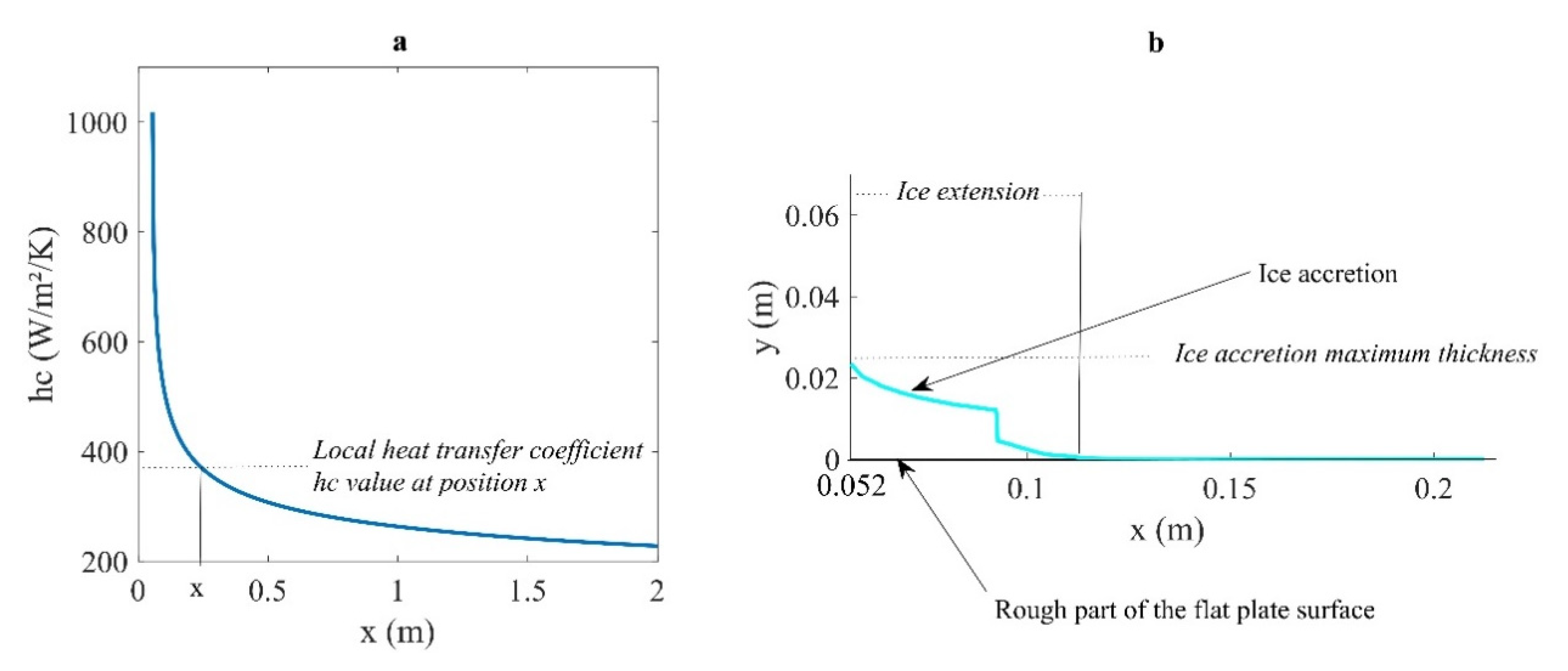
2.1. Convective Heat Transfers over a Rough Flat Plate

For an iced wing, the quasi-random and unknown characteristics of surface roughness introduce uncertainties in the RANS model. The initial uncertainty on roughness characteristics propagates throughout the thermal correction and ice accretion models, leading to uncertain ice accretion characteristics. Similarly to the previous work of Dukhan et al. [14], a rough flat plate geometry is used to model an airfoil, neglecting the pressure gradient effects on the flow. The flat plate represents the upper part of the airfoil, that was unrolled and retains the curvilinear impinging water droplet collection efficiency of the airfoil, as shown on Figure 1a. These assumptions allow for the computing of an ice accretion similar to what is seen on the airfoil, but neglect the curvature effects. Neglecting the curvature effects will produce a slightly underestimated ice thicknesses compared to a curved airfoil. In addition, the absence of positive pressure gradient will increase the boundary layer thickness. This flat plate simplification should not impact the study conclusions, since the sensitivity is ultimately monitored, and not the absolute ice thickness. The epistemic uncertainty is illustrated by two different roughness characteristics (see Figure 1b). Given their geometrical differences, these patterns lead to different convective heat transfer coefficients (see Figure 1c), which in turn cause differences in the characteristics of ice accretions (see Figure 1d).
The database needed to obtain the metamodels relies on RANS simulations. The geometry used in the present work is a 2-m-long horizontal flat plate. This geometry is commonly used in CFD validation [35], and the mesh size is selected according to a grid study presented in [19]. The 2D mesh of the domain consists of a structured domain of 137 by 97 cells with 114 points on the flat plate surface. The growth rate in the direction perpendicular to the plate is 1.3, and the y+ value is between 0.45 and 1.35. In a rough configuration, with this mesh, the difference with the experimental results of Hosni et al. [13] for the Stanton number evaluation was less than 7% for both the HAX and 2PP thermal correction models. In addition, the flat plate configuration was extensively studied both numerically [36] and experimentally [14] in the context of aircraft ice accretion studies. The complete 2.33 m by 1 m domain is sketched in Figure 2. The leading edge of the flat plate is located 0.33 m downstream of the domain inlet.

2.2. Air Mathematical Models

The compressible flow field coming through the inlet boundary of Figure 2 is at Mach 0.2. The Reynolds number based on the length of the plate is 9 million. The Boeing correction for roughness [37] and the thermal correction models are implemented in the Spalart-Allmaras turbulent model of the SU2 6.2.0 solver [19,35]. To obtain the convective heat transfer, the surface temperature is set to 273.15 K, while the ambient air is at 262.04 K. In accordance with the experimental set-up of Dukhan et al. [14], the first 5.2 cm of the plate are unheated, adiabatic and smooth. This starting length allows the boundary layer at the beginning of the rough zone to have a thickness of 1.83 mm.
Two RANS thermal correction models are alternatively used: the HAX model [18] and the 2PP model [19]. Mainly, these models quantify the shift ΔT+ of the nondimensional wall temperature in the thermal boundary layer induced by surface roughness. This shift was first observed for the velocity profile, further denoted as Δu+ [38].
The temperature shift ΔT+ is modelled by increasing the turbulent Prandtl number Prt by an additional ΔPrt in the near-wall region. For the HAX model [18], the Prandtl number correction ΔPrt is a function of the velocity shift Δu+, the normal coordinate to the wall y, the roughness height k, the equivalent sand grain roughness ks and a non-dimensional corrected surface ratio Scorr [39]. This computation only applies in the region located fewer than five times the roughness height away from the wall (i.e., y/k < 5).
Δ P r t = ( A ( Δ u + ) 2 + B Δ u + ) exp ( y / k )  
with:
A = ( 0.0155 0.0035 S c o r r ) ( 1 e 12 ( S c o r r 1 ) )
B =   0.08 + 0.25 e 10 ( S c o r r 1 )
Δ u + =   1 κ · log ( 1 + R e s exp ( 1.3325 ) )
The 2PP model [19] depends only on two parameters, k and ks:
Δ P r t =   g × 0.07083 × R e s 0.45 × P r 0.8 × exp ( y k )
In Equations (4) and (5), the roughness Reynolds number Res is defined as uτks/v. Finally, g = 1 if Res ≥ 70; g = ln ( R e s ) ln ( 5 ) ln ( 70 ) ln ( 5 ) if 5 < Res < 70 and g = 0 if Res ≤ 5.

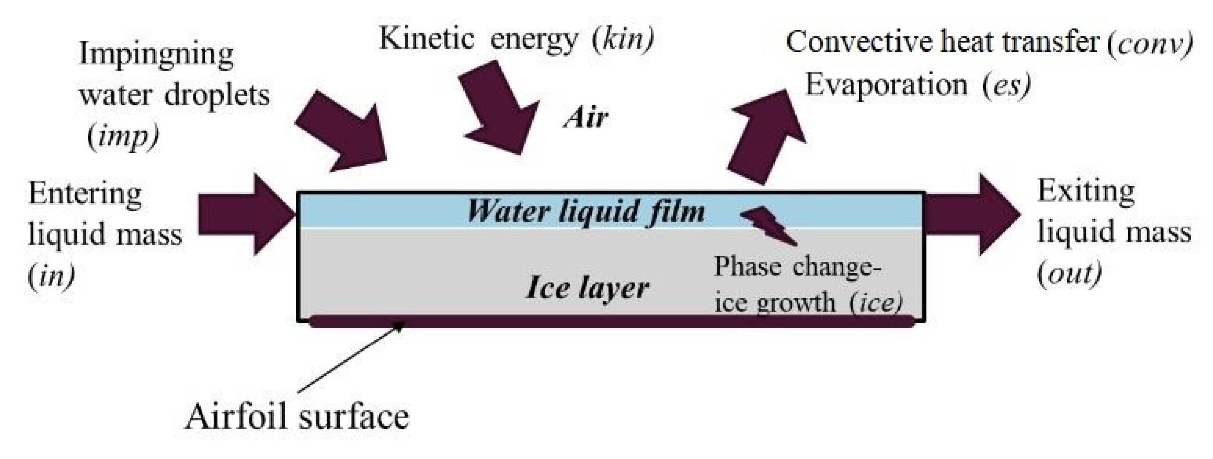
2.3. Ice Accretion Model

Once the heat transfer along the flat plate is known, the ice accretion simulations can be performed. To compute the 2D ice accretions, the Messinger approach is used [6,7]. The basis of this approach is to compute the ice growth rate in a control volume using a mass and an energy balance. The control volume and the contributions to the balances are illustrated in Figure 3.
The mass balance (see Equation (6)) and the energy balance (see Equation (7)) are given by the following set of two equations:
m ˙ i n + m ˙ i m p m ˙ i c e m ˙ e s m ˙ o u t = 0
Q ˙ c o n v + Q ˙ e s + Q ˙ i m p Q ˙ k i n Q ˙ i c e Q ˙ i n = 0
The subscripts appearing in Equations (6) and (7) are defined in Figure 3. More details on the terms involved and the resolution procedure are given in the literature [8,40]. The convective heat transfer, whose coefficient is obtained by the models involved in the previous two subsections, has the general expression given by Equation (8):
Q ˙ c o n v =   h c ( T w T r e c )
with the recovery temperature given by:
T r e c =   T ( 1 + P r 1 / 3 · γ 1 2 M 2 )
The collection efficiency over a NACA0012 airfoil was applied on the flat plate surface and is shown in Figure 4, where s represents the curvilinear abscissa along the airfoil surface, and c represents the chord. The air freestream velocity is 64.9 m/s, the liquid water content is 1.3 g/m3, the droplet diameter is 20 μm and the angle of attack is 0°. Only the upper part of the airfoil, studied through the flat plate representation, is plotted. Note that the plot of Figure 4 is translated for the simulations to have s/c = 0 at the very beginning of the rough zone (at x = 5.2 cm), to have a nonzero boundary layer thickness representative of an airfoil stagnation point.
The icing model presented was successfully verified in previous studies [41], and the ice accretion dependency on the roughness parameters was preliminarily highlighted [8]. The ice thickness is linked to the ice accretion mass, through the ice density of 917 kg/m3, and the exposure time was fixed to 480 s for this work.

3. Uncertainty Quantification and Sensitivity Analysis Method

UQ is used to evaluate the ice accretion uncertainties caused by the heat transfer model parameters in the presence of surface roughness and to identify the most influential parameters. In this section, the uncertain parameter sampling and the NIPCE metamodeling are first depicted, followed by the Sobol indexes definition. In this work, the expression “output of interest”, denoted as Yi, refers to either one of the following features: (1) the local value of the convective heat transfer coefficient at a specified point or (2) the ice accretion characteristics: maximum thickness or ice extension.

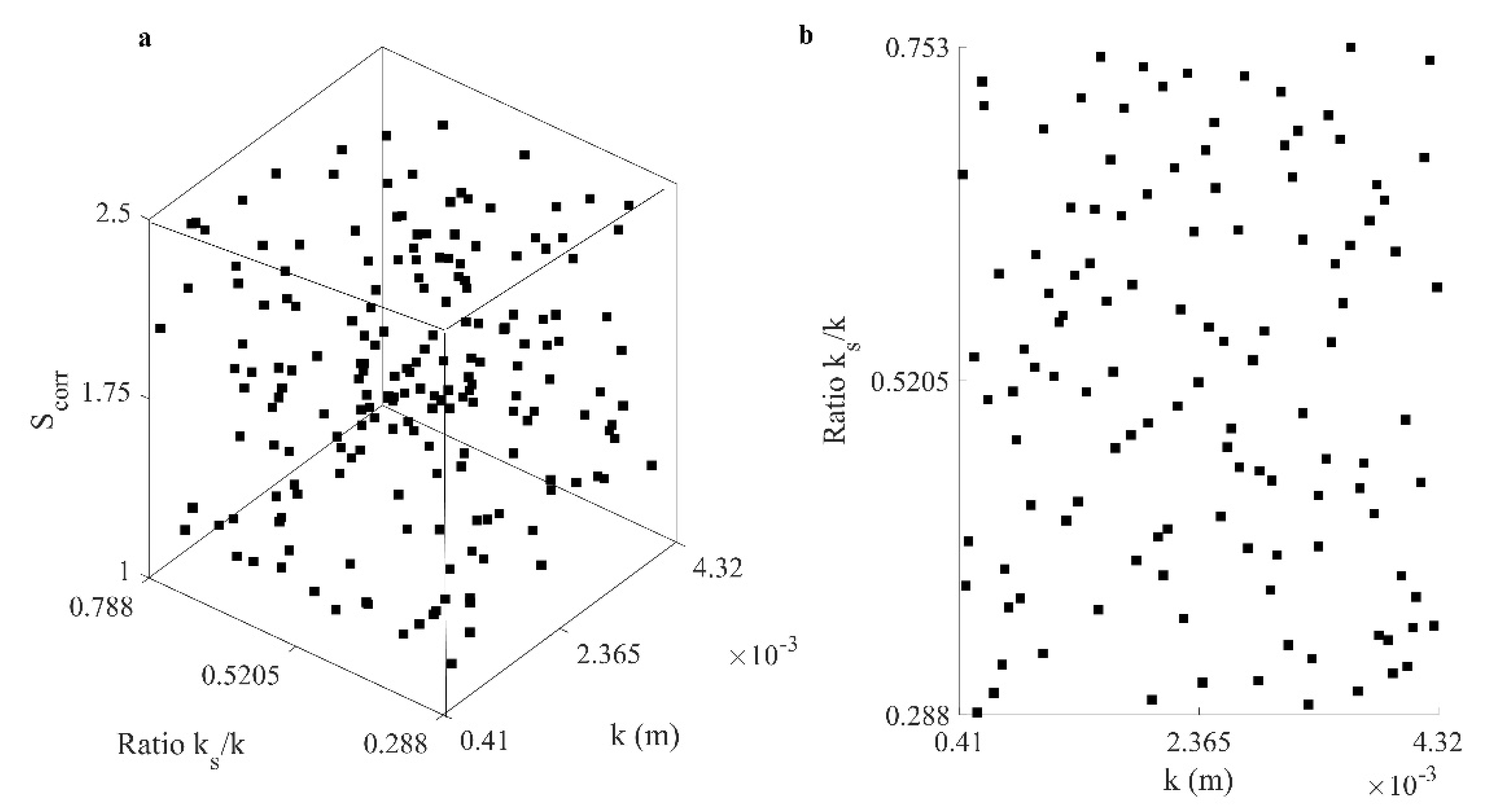
3.1. Uncertain Parameter Sampling and Metamodel

The UQ analysis is used to determine how the roughness’ epistemic uncertainty can impact the PDFs of the ice accretion characteristics. The uncertain inputs of the thermal correction models’ parameters are the roughness height k, its ratio with the equivalent sand grain roughness ks/k and the corrected surface ratio Scorr for the HAX model [18] and k, ks/k for the 2PP model [19]. The choice of the ratio ks/k instead of ks alone comes from the fact that k and ks are linked, for example, with the Dirling relation [25].
The roughness height k was experimentally studied in the literature. For example, Dukhan et al. [14] give a range of variations between 0.41 mm and 4.32 mm on a flat plate measuring 0.458 m by 0.458 m, at a Reynolds number of 2,000,000. These values correspond to the roughness elements observed in different atmospheric conditions, and which led to different surface roughness types. The parameter ks is taken from Fortin [17], who reviewed the validation test cases used for the LEWICE software [42] and concluded on a range of variations for ks between 0.309 mm and 1.247 mm for airfoils with a chord varying between 53.3 cm and 91.4 cm. Both of these ranges for k and ks are maintained in the present study and lead to a ks/k ratio ranging between 0.288 and 0.753. The last input parameter, Scorr, is taken from Aupoix and has a value between 1 and 2.5 [18]. For all the parameters, a uniform PDF between the margins given above is assumed. Although other values are possible in practice, Table 1 gives the distributions used in this study.
With the range of distribution of each parameter defined, the input parameters can be sampled by Latin Hypercube Sampling (LHS), which is one of the methods commonly used to obtain random, but homogeneously spread, sample points [43]. The HAX model has 190 sample simulations and the 2PP model 120, for their respective analyses, as shown in Figure 5. These sample size ranges are in agreement with the literature, which gives a sample size between 160 and 200 for a three-input model [25]. For instance, Solaï et al. used a sample of 115 simulations for their analysis with four input parameters [44].
The sampling presented gives triplets (HAX model) or doublets (2PP model) of roughness parameters that are used as inputs for the RANS simulations. The database of convective heat transfer coefficients and ice accretion characteristics allows for the construction of the metamodels.
The framework used for the UQ analysis, as well as for the subsequent sensitivity analysis, is the UQLab suite [20]. To be able to generate a large number of results (i.e., up to several thousand for the sensitivity analysis) without the need to run additional RANS simulations, three metamodels constructed from the database are used, as shown in Table 2. A metamodel can be represented as a function M estimating the output of interest Yi from the input vector X, whose components are Xj.
The method retained to create the metamodels is the NIPCE [21]. This existing metamodeling tool is frequently used in UQ, and the present work specifically applies it to the UQ for roughness study in aircraft icing. This method is suitable for models with two and three input parameters. The general expression of a NIPCE metamodel is given by Equation (10):
Y i = M ( X ) =   α y α × ψ α ( X )  
When generating a metamodel, the leave-one-out (LOO) error value allows an estimation of the metamodel quality. The LOO value, based on the mean square error between the observed and predicted values, quantifies the ability of the metamodel to predict an output value close to what the RANS computation would have calculated [21]. The computation of the LOO error relies on the cross-validation technique. For an N-sample design, the main aspect of the LOO calculation is to create N metamodels Mi, which are constructed on the CFD database where the ith simulation was dropped, leaving N-1 sample points. The difference between the predicted value of the dropped sample by Mi and its real CFD value allows the computation of the LOO error [45] as in Equation (11).
L O O =   i = 1 N ( Y ( i ) M i ( X ( i ) ) ) 2 i = 1 N ( Y ( i ) Y ¯ ) 2
In Equation (11), X(i) and Y(i) represent the input parameters of the ith CFD sample simulation and the corresponding CFD output, respectively. Finally, Y ¯ is the mean value of the output of interest on the sample dataset. The LOO error is a common tool frequently used in metamodeling application. For instance, Jung et al. extensively used the LOO error for anti-icing performance metamodeling for engine intake [46].

3.2. Sobol Indexes Definition

The purpose of a sensitivity analysis is to identify the uncertain parameters that contribute the most to the variations observed on Yi [26]. Based on the results of the metamodels, the sensitivity of each Yi to the Xi is quantified. The Sobol sensitivity indexes are based on the decomposition of the total variance of Yi. The first-order Sobol index for Xi and the second-order Sobol index for Xi and Xj are defined by Equations (12) and (13), respectively:
S i =   V ( Y ) E ( V ( Y | X i ) ) V ( Y )
S i , j =   V ( Y ) E ( V ( Y | X i ,   X j   ) ) V ( Y )
Finally, for a generic study with three input parameters (i, j, k), the total Sobol index for the parameter i is:
S T i = 1 ( S j + S k + S j , k )
According to Chan et al. [28], a parameter with a total Sobol index greater than 0.8 can be considered as “very important”, with the total Sobol index between 0.5 and 0.8 as “important”, between 0.3 and 0.5 as “unimportant” and “negligible” with an index below 0.3. Consequently, in the present icing application, a total Sobol index close to 1 characterizes an input parameter having a big effectiveness and influence on the ice accretion.
To study the impact of the temperature on the ice accretion sensitivity, the Sobol indexes are computed in two distinct sets of tests. First, the Sobol indexes are estimated on metamodels M1, M2 and M3 as described in Table 2, with the roughness parameters as the only uncertain inputs. For the second set of tests, the temperature is added as an uncertain input parameter. Along with the roughness uncertain parameters of ice accretion metamodels M2 and M3, the freestream temperature T is added as an epistemically uncertain parameter varying uniformly between 261.5 K and 262.5 K. This last series of tests with an uncertain temperature is used to determine if ice accretion is more sensitive to the roughness uncertainty than to the temperature uncertainty.

4. Results and Discussion

With the RANS and the ice accretion models defined, the UQ and Sobol indexes can be applied to study the ice accretion uncertainties over a flat plate. For the outputs of interest, the goals are to evaluate the PDFs and the level of influence of the roughness parameters. For each metamodel and each thermal correction model, the following aspects retain attention: (i) the quality of the metamodel, quantified by the LOO error; (ii) the PDF of the outputs of interest, with the 95% confidence intervals; and (iii) the sensitivity of the outputs of interest to the input parameters, described by the Sobol indexes. For concision, one relevant figure is shown for each aspect listed, and the remaining data for all possible metamodel/thermal correction model combinations are summarized in tables.
The outputs of interest listed in Table 2 are illustrated on Figure 6. Figure 6a shows the outputs of interest on a plot of the convective heat transfer coefficient versus the x position on the flat plate surface. Figure 6b shows the outputs of interest on a graphical representation of an ice accretion. Note that the zone of interest is only the rough part of the flat plate, beginning at x = 5.2 cm.
All the sample simulations will give the same global trends, as observed on Figure 6, with variations induced by the roughness from one sample to another. The convective heat transfer coefficient (Figure 6a) will present a maximum value at the stagnation point before decreasing when traveling downstream along the flat plate. For the ice accretion shape (Figure 6b), the maximum thickness will be at the stagnation point, corresponding to the location of maximum collection efficiency (see Figure 4). The thickness will decrease along the plate with the decrease of the collection efficiency. In addition, the runback water will end up freezing, giving the observed step, located, in the example of Figure 6b, at x = 0.08 m. The step is due to the fact that no more liquid water runs back further downstream.

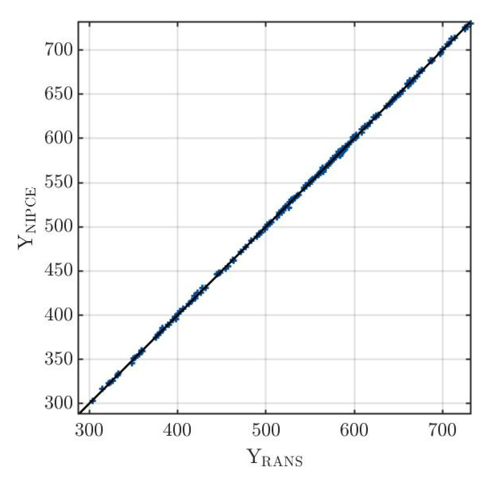
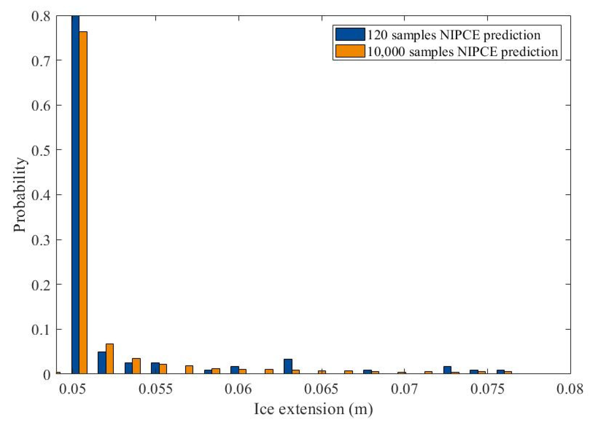
4.1. Precision of the Metamodels Generated

Prior to looking at the LOO error value, the precision of the metamodel may be visualized by plotting the NIPCE prediction for the set of input parameters used for the RANS simulations versus the actual RANS calculated value. Figure 7 shows this scatter plot for the metamodel M1 of the HAX model. YRANS represents the RANS-calculated values of the local convective heat transfer coefficient at x = 11.36 cm (with x = 0 taken at the very beginning of the flat plate), while YNIPCE represents the corresponding values predicted by the metamodel. The points for the 190 sample simulations are plotted and show that the metamodel M1 for the HAX model has a good precision, with an absolute mean error between the RANS-calculated values and the NIPCE-predicted values of 0.90 W/m2/K and a linear regression coefficient of 0.9999. This regression coefficient value is higher than the ones commonly accepted in the literature for sensitivity analysis [32]. The LOO error for this metamodel, M1, at x = 11.36 cm is 4.25 × 10⁻⁴. The local position x = 11.36 cm was chosen among the 114 possible surface grid points to illustrate the behavior of the metamodel.
The trend shown in Figure 7, with all the scatter points homogeneously packed close to the identity line, suggests a metamodel making accurate predictions. Checking the precision of all the metamodels leads to the LOO errors presented in Table 3.
The values presented in Table 3 show that the convective heat transfer coefficient is well predicted by the metamodels: the LOO error for both HAX and 2PP is in the neighborhood of 10−4, which is an acceptable value that leads to a precision similar to the one of Figure 7. Nevertheless, the 2PP model has a more predictable behavior than its HAX counterpart. The values show a LOO error two to four times smaller than the one of the HAX model for a given metamodel. For the ice accretion characteristics, the HAX model shows a loss of predictability since the LOO errors rise to the 10−3 to 10−2 range of values. On the other hand, the 2PP model still presents a well-predictable icing behavior with the LOO error once again in the 10−4 magnitude.

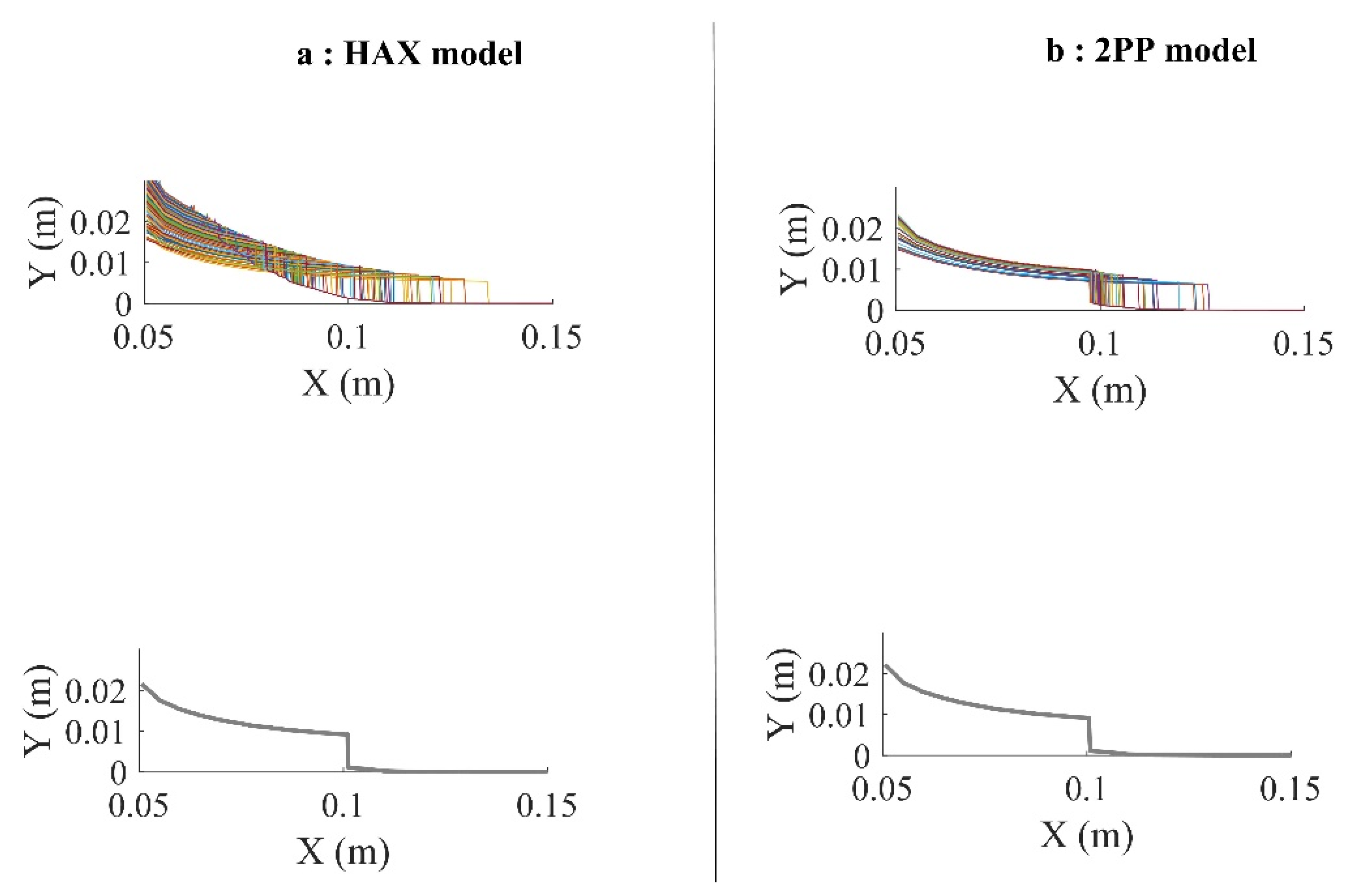
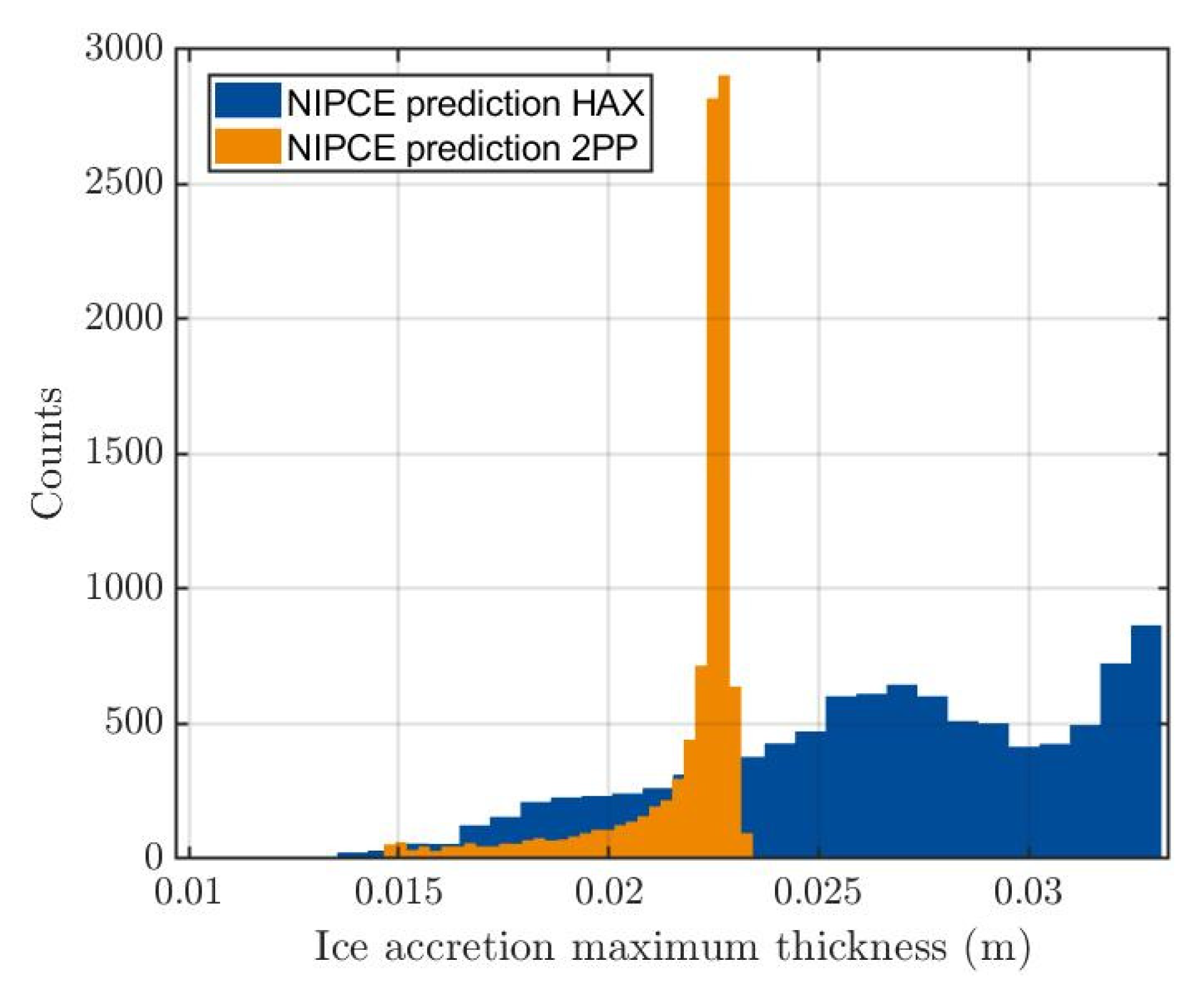
4.2. Outputs of Interest PDFs

The metamodel-generated databases allow the computation of the outputs of interest PDFs. Figure 8 shows all the ice accretion shapes obtained for (a) the HAX model and (b) the 2PP model. Additionally, for each of the models, one ice accretion chosen among the set is plotted alone for clear visualization. Each of the colored lines on the top charts of Figure 8 represents one specific accretion obtained with one particular sample run. For the single plotted accretions, the specific roughness parameters for the HAX model (a) are k = 1.14 mm, ks/k = 0.599 and Scorr = 1.17, and for the 2PP model (b), k = 2.07 mm and ks/k = 0.385. The general trend illustrated in Figure 6, with a step observed in the accretion, is visible for all the sample accretions. Figure 8 shows that varying the roughness parameters changes the position of the step, which characterizes the ice extension along the surface.
Using all 190 (HAX model) or 120 (2PP model) data sets allows for the computing of the NIPCE-predicted PDF of the outputs of interest. The NIPCE allows for an increase in sample size, but the PDF is similar to the PDF predicted, with a sample size of 190 or 120. To verify this for the 2PP model, a sample of 10,000 doublets (k, ks/k) was generated with the Latin Hypercube Sampling, and the NIPCE metamodel applied to the sample. The PDFs of the 120 and 10,000 NIPCE predictions are shown together in Figure 9, where the bars’ heights are scaled by the total number of predictions for each case (i.e., 120 and 10,000, respectively).
Figure 9 shows a similar trend. A closer analysis allows for the determination of the PDF of the data in the figure. The fitted normal distributions, associated to the histograms of Figure 9, have their parameters μ and σ summarized in Table 4, with the 95% confidence intervals in square brackets. The first column in Table 4 gives the parameters for the NIPCE prediction histogram of Figure 9 obtained with 120 samples, and the second column gives the PDF parameters as extracted from the prediction with 10,000 samples. Note that the NIPCE metamodel obtained, defined by a polynomial as in Equation (10), in both the sample sizes (120 and 10,000), is of degree 7.
The parameters in Table 4 show that the NIPCE prediction M3 with 120 samples matches closely the prediction obtained with 10,000 samples. The PDF parameters of the NIPCE response only change by a magnitude of 10−4 for μ and 0.0005 for σ. This aspect shows that the sample size of 120 was already enough to estimate the PDF of the output with a good precision. Nevertheless, the confidence intervals are reduced with the increase of the sample size: the confidence interval on μ for 120 samples is 1.9 mm wide, while it is 0.3 mm wide for the 10,000 samples. By applying the relation from [25], with an oversampling ratio of 3 for two uncertain parameters and a NIPCE of degree 7, the minimum sample size required for the problem is 108. This confirms, in addition to the graphical visualization, that the sample size of 120 is enough. This characteristic of having a high enough precision with the RANS sample size is also verified for all the other metamodels. To ensure a small confidence interval, the results obtained for a 10,000 sample size are kept. The normal distributions obtained for each metamodel with the NIPCE prediction with 10,000 samples are summarized in Table 5.
The data in Table 5 show that each thermal correction model predicts slightly different output PDFs for the same metamodel. The μ values in Table 5 show that, statistically, changing from the HAX to the 2PP thermal correction model leads to a 21% variation in the heat transfer coefficient. This change in the heat transfer coefficient then leads to a 17% variation in the ice maximum thickness and only 1.8% of change in the ice extension. The standard deviation σ allows us to estimate the relative uncertainty and how the observed values spread around the mean μ. For a normal distribution, 99.7% of the data are in the range [μ − 3σ; μ + 3σ]. The σ values in Table 5 suggest a larger uncertainty on the outputs for the HAX model compared to the 2PP model. For the ice extension, the relative uncertainty in the 99.7% range [μ − 3σ; μ + 3σ] is about 36% for the HAX model and 27% for the 2PP model. The same calculation for the maximum ice thickness leads to a relative uncertainty of 52% for the HAX model and 23% for the 2PP model. As expected, these uncertainties on the accretion find their origin in the heat transfer uncertainties, which are 58% and 19% for the HAX and 2PP models, respectively. As an example, Figure 10 shows the difference in the distributions predicted by metamodel M2 for the maximum ice thickness. The difference between the distributions predicted for the HAX model (orange) and the 2PP model (blue) is noticeable. The larger standard deviation for the HAX model is clearly visible, with a larger spread of the values around the mean compared to the 2PP model.
Figure 10 shows that the two thermal correction models predict different maximum ice thickness ranges: the 2PP model gives ice accretions with thicknesses of up to about 23 mm, while the HAX model predicts thicknesses of up to 33 mm.

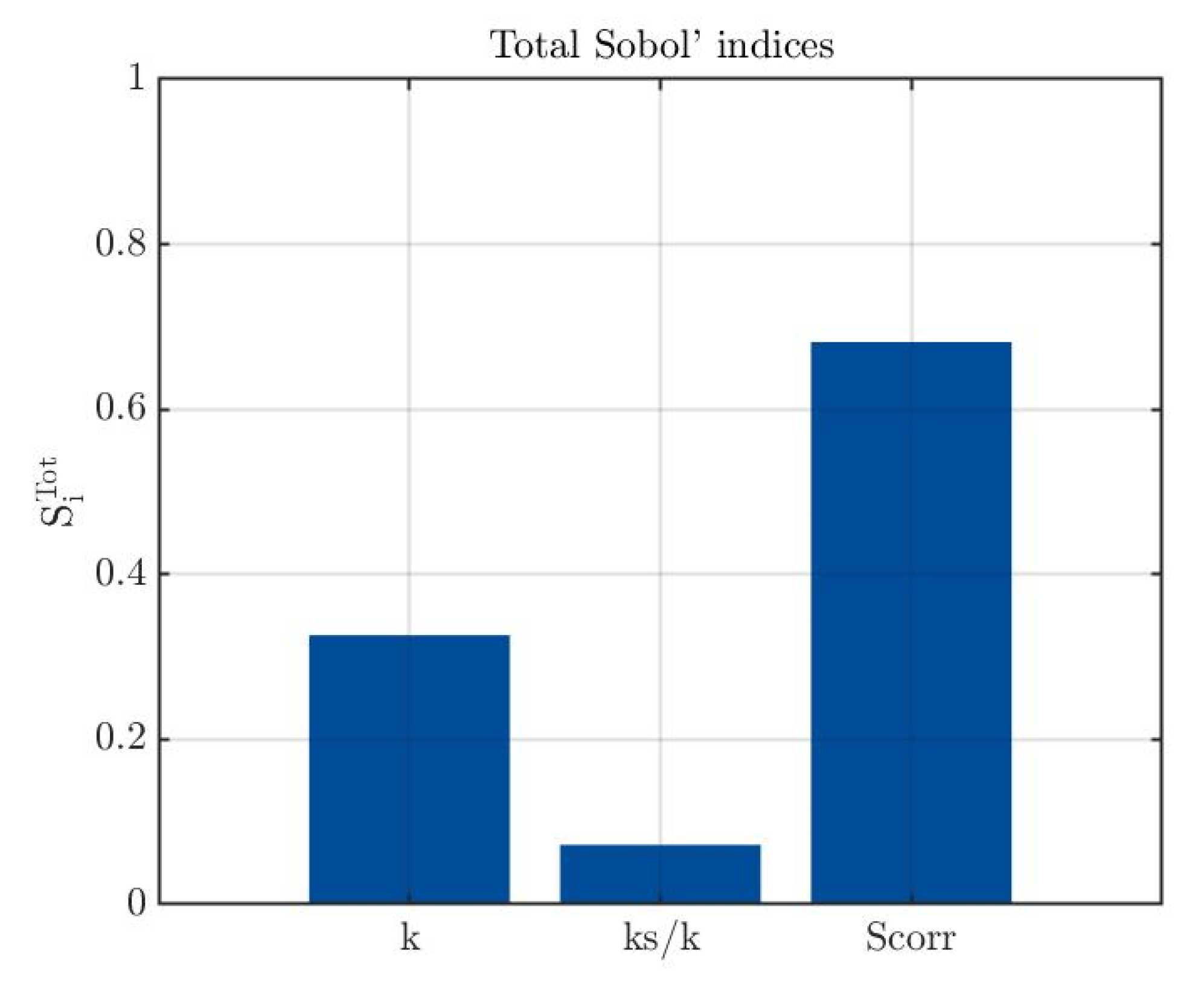
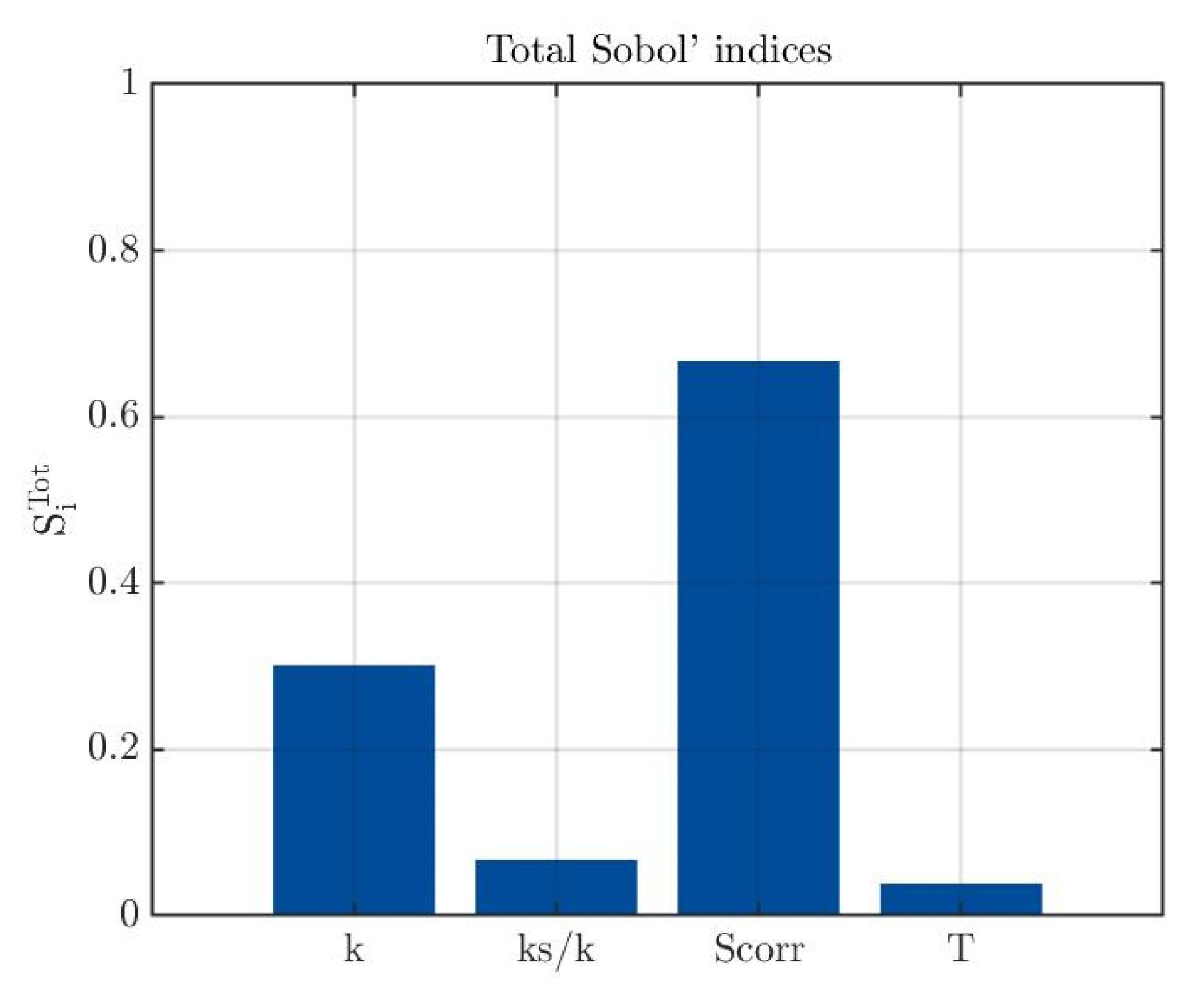
4.3. Sensitivity Analysis: Calculation of the Sobol Sensitivity Indexes

4.3.1. Sensitivity to the Roughness Parameters

With the metamodels generated, the Sobol sensitivity indexes are evaluated for each input parameter. The 2PP model, with two input parameters, allows the computation of the Sobol indexes up to order 1, while the HAX model, with three input parameters, allows Sobol indexes of order 2. Figure 11 shows the Sobol indexes for the metamodel M2, evaluating the maximum thickness of the ice accretion and the HAX thermal correction model. The values of the total Sobol indexes obtained for each metamodel are shown in Table 6. In Table 6, three positions have been chosen for the metamodel M1, to highlight the differences of sensitivity when traveling on the flat plate.
The results in Figure 11 and Table 6 show, for the HAX model, that the parameter Scorr has the largest impact on every output of interest: Scorr contributes up to 68% to the variability of the maximum ice thickness and 82% for the ice extension. For the 2PP model (see Table 6), the roughness height k has the greatest influence on the outputs of interest as compared to the ratio ks/k, going up to about 91%. The results observed for the 2PP model, where k has a greater influence than the ratio ks/k, are also observed for the HAX model. According to the classification given by Chan et al. [28], Scorr is an important or very important parameter for every metamodel, while k and the ratio ks/k are negligible or unimportant for the HAX thermal correction model. For the 2PP thermal correction model, k is very important compared to the ratio ks/k, which is negligible. These results show that in the case of the HAX model, Scorr needs to be carefully quantified prior to launching a simulation, since the outputs of interest are the most sensitive to its value. The same conclusion can be drawn for the parameter k when using the 2PP model. Looking at the values in Table 6, it can be observed that the roughness height k sees its level of influence decreasing as it gets away from the leading edge with the 2PP thermal correction. This observation is done by comparing the Sobol indexes from metamodel M1 at x = 11.36 cm and further away at x = 14.29 cm and x = 27.48 cm, where the Sobol index for k decreases. Meanwhile, the Sobol indexes for ks/k increase while traveling away from the leading edge. For the HAX model, the Sobol indexes for all three uncertain parameters remain quite steady when traveling downstream.

4.3.2. Sensitivity of the Ice Accretion to the Roughness Parameters and the Freestream Temperature

To highlight the importance of roughness parameters on the ice accretion shape compared to the freestream temperature, the freestream temperature T is now added as an epistemically uncertain variable, varying randomly between 261.5 K and 262.5 K, and the Sobol indexes are computed. For these tests, the parameters are summarized in Table 7.
The new metamodels, with an increased number of uncertain input parameters, have a subscript “T” to avoid confusion. For the sake of concision, the LOO errors and outputs’ PDFs of metamodels M2T and M3T are not displayed, but the precision is of the same order of magnitude as that of metamodels M2 and M3. The Sobol indexes of metamodel M2T for the HAX thermal correction model are displayed in Figure 12.
Figure 12 shows that the temperature has a minor impact on the sensitivity of the ice accretion’s maximum thickness. When comparing with Figure 11, it is also possible to note that the level of influence of the roughness parameters remains almost the same despite the addition of the temperature as uncertain. This negligible influence of the temperature is also observed for the other combinations of metamodel/thermal correction model, as summarized in Table 8.
The results in Table 8 show that for every metamodel and thermal correction model, the temperature is the least influent parameter. For the HAX thermal correction model, T is completely negligible, while for the 2PP model it has a greater impact, closer to ks/k, but still far behind the level of influence of the roughness height k and still below 0.3. These results highlight the importance of the roughness model in the simulation, whose parameters have to be carefully selected, since their variation leads to bigger changes to the ice accretion shape than the temperature variation within 1 K. This relative importance of roughness on the accretion sensitivity compared to other factors related to ambient conditions has also been noticed in the literature. In [32], Raj et al. showed that the roughness plays a bigger role in the accretion shape than the ice density, the droplet distribution and the evaporation.
The results show that the methodology retained is well suited to the ice accretion, since the NIPCE satisfactorily predicts the behavior of the output of interest. The NIPCE metamodeling gave fast responses and facilitated the analysis for the aircraft icing study. The results obtained using the NIPCE tool allow for a direct observation of the key features of the accretion’s characteristics when roughness parameters are varying. Following that, the sensitivity analysis allowed us to determine that the outputs of interest are very sensitive to Scorr when using the HAX model, and to the roughness height k when using the 2PP model.
The ranges of the uncertain roughness parameters come from the literature, and uniform PDFs have been chosen. Changing the ranges and/or the PDFs might impact the results. Other types of metamodels can also be investigated. A similar study can also be conducted around an airfoil to highlight the effects of curvature and pressure gradient effects on the results. Furthermore, k, unlike Scorr and ks/k, is linked to the skin friction coefficient, which is seldom available and known for an iced surface.

5. Conclusions

This paper has introduced an efficient methodology to quantify the sensitivity of the ice accretion characteristics to the thermal correction parameters on a rough flat plate. The objective of the paper to quantify the ice shape uncertainty and identify the key roughness parameters leading to this uncertainty was reached. The main parts of the methodology were the metamodeling process, using the Non-Intrusive Polynomial Chaos Expansion (NIPCE), and the sensitivity study computing the Sobol sensitivity indexes. The NIPCE metamodeling tool gave entire satisfaction regarding accuracy and quickly computed results with up to several thousand inputs. These features highlighted NIPCE’s suitability for the study, despite its novel usage for aircraft icing with roughness analysis. The study allowed a comparison of two thermal correction models: the HAX model, with three input parameters, and the 2PP model, with two input parameters. The predicted ice accretion’s maximum thickness is very sensitive to the choice of the thermal correction model and its respective parameters. Switching from the HAX to the 2PP thermal correction induces a 17% change in the maximum ice thickness. This aspect is mainly due to the impact of the thermal correction on the convective heat transfer, which is changed up to about 20%. In addition, the standard deviation study highlighted a larger relative uncertainty on the accretion for the HAX model, which can reach 52% on the ice maximum thickness compared to the uncertainty of 23% of the 2PP model. It was also concluded from the Sobol sensitivity indexes that the most influential parameter for the HAX model is Scorr, which is responsible of 68% and 82% of variations on the ice accretion’s maximum thickness and extension, respectively. For the 2PP model, the roughness height k is the most sensitive parameter, responsible for about 90% of the changes in ice thickness and extension. To improve the rough turbulence models, it seems necessary to reinforce the experimental databases by precisely measuring the heat transfer variations induced by typical ice roughness. The present work shows that the precise knowledge of the heat transfers associated to a specific roughness pattern is key to ensuring reliable numerical icing predictions. Future investigations will be conducted to apply the same methodology to an airfoil.

Author Contributions

Conceptualization, K.I.; methodology, K.I.; validation, K.I., F.M. and H.B.; data curation, K.I.; writing—original draft preparation, K.I.; writing—review and editing, F.M. and H.B.; visualization, K.I.; supervision, F.M. and H.B. All authors have read and agreed to the published version of the manuscript.

Funding

This research received no external funding.

Data Availability Statement

The data presented in this study are available on request from the corresponding author.

Acknowledgments

The authors would like to thank the TOMATO Association (Aéroclub de France), Paris, France; the Office of the Dean of Studies, ÉTS, Montréal, Canada; and SubstanceÉTS, Montreal, Canada. CFD computations were made on the Cedar supercomputer from Simon Fraser University, managed by Calcul Québec and Compute Canada.

Conflicts of Interest

The authors declare no conflict of interest.

Nomenclature

Cffriction coefficient
Cpheat capacity at constant pressure of air (J/(kg·K))
E(V(Y|Xi))mean of the conditional variance for Xi fixed
E(V(Y|Xi, Xj))mean of the conditional variance for Xi and Xj fixed
gparameter for the 2PP formulation
hcconvective heat transfer coefficient (W/m2/K)
hwwall heat flux (W/m2)
kroughness height (m)
ksequivalent sand grain roughness (m)
m ˙ mass rate (kg/m2/s)
M(X)metamodel function
MaMach number
Prlaminar Prandtl number
Prtturbulent Prandtl number
Q ˙ specific energy rate (W/m2)
Resroughness Reynolds number
Scorrwetted corrected surface ratio
Sifirst-order Sobol index
Si,jsecond-order Sobol index
STitotal Sobol index
Ttemperature (K)
T+non-dimensional temperature
Trecrecovery temperature (K)
Twwall temperature (K)
uvelocity (m/s)
u+non-dimensional velocity
uτshear velocity (m/s)
Vvariance
Xiinput component
ycoordinate normal to the wall (m)
Yioutput of interest
yαcoefficients for the PCE decomposition
αmulti-index for the PCE decomposition
γheat capacity ratio of air
ΔPrtturbulent Prandtl number shift
ΔT+non-dimensional temperature shift
Δu+non-dimensional velocity shift
κVon Karman constant
νkinematic viscosity (m2/s)
τwwall shear stress (N/m2)
ψα(X)multivariate polynomial for the PCE decomposition
Subscripts
convconvective
esevaporation/sublimation
iceice growth
impimpinging water
inentering runback water
kinkinetic energy
outexiting runback water
Roughrough surface
Smoothsmooth surface
wwall

References

  1. Tagawa, G.D.; Morency, F.; Beaugendre, H. CFD study of airfoil lift reduction caused by ice roughness. In Proceedings of the 2018 Applied Aerodynamics Conference, Atlanta, Georgia, 25–29 June 2018. [Google Scholar] [CrossRef]
  2. Jones, S.M.; Reveley, M.S.; Evans, J.K.; Barrientos, F.A. Subsonic Aircraft Safety Icing Study; Center, N.L.R., Ed.; NASA: Hampton, VA, USA, 2008; p. 45.
  3. Bragg, M.B.; Broeren, A.P.; Blumenthal, L.A. Iced-airfoil aerodynamics. Prog. Aerosp. Sci. 2005, 41, 323–362. [Google Scholar] [CrossRef]
  4. Saeed, F. State-of-the-Art Aircraft Icing and Anti-Icing Simulation. ARA J. 2002, 2000, 106–113. [Google Scholar]
  5. Rto/Nato, Ice Accretion Simulation Evaluation Test; Research and Technlology Organization: Neuilly sur Seine, France, 2001; p. 32.
  6. Messinger, B.L. Equilibrium Temperature of an Unheated Icing Surface as a Function of Air Speed. J. Aeronaut. Sci. 1953, 20, 29–42. [Google Scholar] [CrossRef]
  7. Lavoie, P.; Pena, D.; Hoarau, Y.; Laurendeau, E. Comparison of thermodynamic models for ice accretion on airfoils. Int. J. Numer. Methods Heat Fluid Flow 2018, 28, 1004–1030. [Google Scholar] [CrossRef]
  8. Ignatowicz, K.; Morency, F.; Beaugendre, H. Numerical simulation of ice accretion using Messinger-based approach: Effects of surface roughness. In CASI AERO 2019; CASI: Laval, QC, Canada, 2019. [Google Scholar]
  9. Cao, Y.; Ma, C.; Zhang, Q.; Sheridan, J. Numerical simulation of ice accretions on an aircraft wing. Aerosp. Sci. Technol. 2012, 23, 296–304. [Google Scholar] [CrossRef]
  10. Newton, E.; James Vanfossen, J.; Poinsatte, G.; Dewitt, K. Measurement of Local Convective Heat Transfer Coefficients from a Smooth and Roughened NACA-0012 Airfoil: Flight Test Data, in 26th Aerospace Sciences Meeting; NASA: Reno, Nevada, 1988.
  11. Poinsatte, P.E.; Fossen, G.J.V.; Witt, K.J.D. Roughness effects on heat transfer from a NACA 0012 airfoil. J. Aircr. 1991, 28, 908–911. [Google Scholar] [CrossRef]
  12. Liu, Y.; Hu, H. An experimental investigation on the unsteady heat transfer process over an ice accreting airfoil surface. Int. J. Heat Mass Transf. 2018, 122, 707–718. [Google Scholar] [CrossRef]
  13. Hosni, M.H.; Coleman, H.W.; Garner, J.W.; Taylor, R.P. Roughness element shape effects on heat transfer and skin friction in rough-wall turbulent boundary layers. Int. J. Heat Mass Transf. 1993, 36, 147–153. [Google Scholar] [CrossRef]
  14. Dukhan, N.; Masiulaniec, K.C.; Witt, K.J.D.; Fossen, G.J.V. Experimental Heat Transfer Coefficients from Ice-Roughened Surfaces for Aircraft Deicing Design. J. Aircr. 1999, 36, 948–956. [Google Scholar] [CrossRef]
  15. Dukhan, N.; Masiulaniec, K.C.; Witt, K.J.D.; Fossen, G.J.V. Acceleration Effect on the Stanton Number for Castings of Ice-Roughened Surfaces. J. Aircr. 1999, 36, 896–898. [Google Scholar] [CrossRef]
  16. Hansman, R.; Yamaguchi, K.; Berkowitz, B.; Potapczuk, M. Modeling of Surface Roughness Effects on Glaze Ice Accretion. J. Thermophys. Heat Transf. 1989, 5. [Google Scholar] [CrossRef] [Green Version]
  17. Fortin, G. Equivalent Sand Grain Roughness Correlation for Aircraft Ice Shape Predictions; SAE International: Warrendale, PA, USA, 2019. [Google Scholar] [CrossRef]
  18. Aupoix, B. Improved heat transfer predictions on rough surfaces. Int. J. Heat Fluid Flow 2015, 56, 160–171. [Google Scholar] [CrossRef]
  19. Morency, F.; Beaugendre, H. Comparison of turbulent Prandtl number correction models for the Stanton evaluation over rough surfaces. Int. J. Comput. Fluid Dyn. 2020. [Google Scholar] [CrossRef]
  20. Sudret, B.; Marelli, S.; Wiart, J. Surrogate models for uncertainty quantification: An overview. In Proceedings of the 2017 11th European Conference on Antennas and Propagation (EUCAP), Paris, France, 19–24 March 2017. [Google Scholar] [CrossRef]
  21. Marelli, S.; Sudret, B. UQLab user manual—Polynomial chaos expansions. In Chair of Risk, Safety and Uncertainty Quantification; ETH: Zurich, Switzerland, 2019. [Google Scholar]
  22. Cinnella, P.; Congedo, P.M.; Parussini, L.; Pediroda, V. Quantification of Thermodynamic Uncertainties in Real Gas Flows. Int. J. Eng. Syst. Model. Simul. 2010, 2. [Google Scholar] [CrossRef]
  23. Weissenbrunner, A.; Fiebach, A.; Schmelter, S.; Bär, M.; Thamsen, P.U.; Lederer, T. Simulation-based determination of systematic errors of flow meters due to uncertain inflow conditions. Flow Meas. Instrum. 2016, 52, 25–39. [Google Scholar] [CrossRef] [Green Version]
  24. Schaefer, J.A.; Romero, V.J.; Schafer, S.R.; Leyde, B.; Denham, C.L. Approaches for Quantifying Uncertainties in Computational Modeling for Aerospace Applications. In Proceedings of the AIAA Scitech 2020 Forum, Orlando, FL, USA, 6–10 January 2020. [Google Scholar] [CrossRef]
  25. Schaefer, J.A.; Cary, A.W.; Mani, M.; Spalart, P.R. Uncertainty Quantification and Sensitivity Analysis of SA Turbulence Model. Coefficients in Two and Three Dimensions. In Proceedings of the 55th AIAA Aerospace Sciences Meeting, Grapevine, TX, USA, 9–13 January 2017. [Google Scholar] [CrossRef]
  26. Saltelli, A.; Ratto, M.; Andres, T.; Campolongo, F.; Cariboni, J.; Gatelli, D.; Saisana, M.; Tarantola, S. Global Sensitivity Analysis: The Primer; John Wiley & Sons: Hoboken, NJ, USA, 2008; Volume 304. [Google Scholar] [CrossRef]
  27. Chen, W.; Jin, R. Analytical Variance-Based Global Sensitivity Analysis in Simulation-Based Design Under Uncertainty. J. Mech. Des. 2005, 127. [Google Scholar] [CrossRef]
  28. Chan, K.; Saltelli, A.; Tarantola, S. Sensitivity Analysis of Model. Output: Variance-based Methods Make the Difference. In Proceedings of the 1997 Winter Conference, Atlanta, Georgia, 7–10 December 1997; pp. 261–268. [Google Scholar] [CrossRef]
  29. Tabatabaei, N.; Raisee, M.; Cervantes, M.J. Uncertainty Quantification of Aerodynamic Icing Losses in Wind Turbine with Polynomial Chaos Expansion. J. Energy Resour. Technol. 2019, 141. [Google Scholar] [CrossRef]
  30. Kato, H.; Ito, K.; Lepot, I. Sensitivity analysis based on high fidelity simulation: Application to hypersonic variable-cycle engine intake design. Int. J. Eng. Syst. Model. Simul. 2010, 2. [Google Scholar] [CrossRef]
  31. Zhu, P.; Yan, Y.; Song, L.; Li, J.; Feng, Z. Uncertainty Quantification of Heat Transfer for a Highly Loaded Gas Turbine Blade Endwall Using Polynomial Chaos. In Proceedings of the ASME Turbo. Expo. 2016: Turbomachinery Technical Conference and Exposition, Seoul, Korea, 13–17 June 2016. [Google Scholar] [CrossRef]
  32. Prince Raj, L.; Yee, K.; Myong, R.S. Sensitivity of ice accretion and aerodynamic performance degradation to critical physical and modeling parameters affecting airfoil icing. Aerosp. Sci. Technol. 2020, 98. [Google Scholar] [CrossRef]
  33. Degennaro, A.M.; Rowley, C.W.; Martinelli, L. Uncertainty Quantification for Airfoil Icing Using Polynomial Chaos Expansions. J. Aircr. 2015, 52, 1404–1411. [Google Scholar] [CrossRef] [Green Version]
  34. Hussain, M.F.; Barton, R.R.; Joshi, S.B. Metamodeling: Radial basis functions, versus polynomials. Eur. J. Oper. Res. 2002, 138, 142–154. [Google Scholar] [CrossRef]
  35. Economon, T.D.; Palacios, F.; Copeland, S.R.; Lukaczyk, T.W.; Alonso, J.J. SU2: An Open-Source Suite for Multiphysics Simulation and Design. AIAA J. 2015, 54, 828–846. [Google Scholar] [CrossRef]
  36. Yanxia, D.; Yewei, G.; Chunhua, X.; Xian, Y. Investigation on heat transfer characteristics of aircraft icing including runback water. Int. J. Heat Mass Transf. 2010, 53, 3702–3707. [Google Scholar] [CrossRef]
  37. Aupoix, B.; Spalart, P.R. Extensions of the Spalart–Allmaras turbulence model to account for wall roughness. Int. J. Heat Fluid Flow 2003, 24, 454–462. [Google Scholar] [CrossRef]
  38. Nikuradse, J. Laws of flow in rough pipes. VDI Forsch. 1933, 4, 63. [Google Scholar]
  39. Radenac, E.; Kontogiannis, A.; Bayeux, C.; Villedieu, P. An extended rough-wall model for an integral boundary layer model intended for ice accretion calculations. In Proceedings of the 2018 Atmospheric and Space Environments Conference, Atlanta, Georgia, 25 June 2018. [Google Scholar] [CrossRef]
  40. Özgen, S.; Canıbek, M. Ice accretion simulation on multi-element airfoils using extended Messinger model. Heat Mass Transf. 2008, 45, 305. [Google Scholar] [CrossRef]
  41. Ignatowicz, K.; Morency, F.; Beaugendre, H. Simulations numériques de changement de phase appliquées au givrage en aéronautique. In Proceedings of the XIVème Colloque International Franco-Québécois en énergie, Baie-Saint-Paul QC, Canada, 6–20 June 2019. [Google Scholar]
  42. Wright, W.B.; Struk, P.; Bartkus, T.; Addy, G. Recent Advances in the LEWICE Icing Model; SAE International: Warrendale, PA, USA, 2015. [Google Scholar] [CrossRef]
  43. Stein, M. Large sample properties of simulations using latin hypercube sampling. Technometrics 1987, 29, 143–151. [Google Scholar] [CrossRef]
  44. Solaï, E.; Beaugendre, H.; Congedo, P.-M.; Daccord, R.; Guadagnini, M. Numerical Simulation of a Battery Thermal Management System Under Uncertainty for a Racing Electric Car. In La Simulation Pour la Mobilité Électrique; NAFEMS: Paris, France, 2019. [Google Scholar]
  45. Blatman, G.; Sudret, B. An adaptive algorithm to build up sparse polynomial chaos expansions for stochastic finite element analysis. Probabilistic Eng. Mech. 2010, 25, 183–197. [Google Scholar] [CrossRef]
  46. Jung, S.; Raj, L.P.; Rahimi, A.; Jeong, H.; Myong, R.S. Performance evaluation of electrothermal anti-icing systems for a rotorcraft engine air intake using a meta model. Aerosp. Sci. Technol. 2020, 106, 106174. [Google Scholar] [CrossRef]
Figure 1. Uncertainty propagation from surface roughness to ice accretion shape.
Aerospace 08 00084 g001
Figure 2. Visual representation of the computational domain.
Aerospace 08 00084 g002
Figure 3. Control volume and energy and mass terms used in the Messinger icing model.
Aerospace 08 00084 g003
Figure 4. Collection efficiency of the upper part of the NACA0012 airfoil as used on the flat plate surface [40].
Aerospace 08 00084 g004
Figure 5. Sample points for (a) the HAX model and (b) the 2PP model obtained by Latin Hypercube Sampling.
Aerospace 08 00084 g005
Figure 6. Outputs of interest for (a) the heat transfer coefficient and (b) the ice accretion.
Aerospace 08 00084 g006
Figure 7. Non-Intrusive Polynomial Chaos Expansion (NIPCE) predicted (M1) vs. Reynolds-Averaged Navier-Stokes (RANS) calculated value for the local heat transfer coefficient at x = 11.36 cm (HAX model).
Aerospace 08 00084 g007
Figure 8. Examples of accretions obtained: (a) HAX model and (b) 2PP model.
Aerospace 08 00084 g008
Figure 9. Comparison between NIPCE predictions for a varying sample size for the ice extension (metamodel M3) and the 2PP model.
Aerospace 08 00084 g009
Figure 10. Differences in predicted distributions between the HAX and 2PP models for metamodel M2 on the 10,000 samples.
Aerospace 08 00084 g010
Figure 11. Total Sobol indexes for metamodel M2 and the HAX thermal correction model.
Aerospace 08 00084 g011
Figure 12. Total Sobol indexes for metamodel M2T and the HAX thermal correction model.
Aerospace 08 00084 g012
Table 1. Summary of the distributions for the input parameters.
Parameter XiMinimumMaximumDistribution
k (mm)0.414.32Uniform
Ratio ks/k0.2880.753Uniform
Scorr12.5Uniform
Table 2. Metamodels generated.
MetamodelInput Parameters XjOutput of Interest Yi
HAX2PP
M1k, ks/k, Scorr, xk, ks/k, xConvective heat transfer coefficient value at position x
M2k, ks/k, Scorrk, ks/kMaximum ice accretion thickness
M3k, ks/k, Scorrk, ks/kIce accretion extension
Table 3. Leave-one-out (LOO) errors for all the metamodels.
MetamodelOutput of Interest YiLOO Error
HAX2PP
M1Heat transfer coefficient value at 11.36 cm4.25 × 10−42.15 × 10⁻⁴
M2Maximum ice accretion thickness4.12 × 10−31.05 × 10⁻⁴
M3Ice accretion extension1.52 × 10−24.49 × 10⁻⁴
Table 4. PDF of normal distribution parameters of Figure 9’s histograms.
120 Samples NIPCE Prediction10,000 Samples NIPCE Prediction
μ = 0.0522 m [0.0512; 0.0531]
σ = 0.0052 [0.0046; 0.0059]
μ = 0.0521 m [0.0520; 0.0522]
σ = 0.0047 [0.0046; 0.0047]
Table 5. Output PDF for each NIPCE prediction on the 10,000 sample size.
MetamodelOutput of Interest YiOutput PDFs’ Parameters
HAX2PP
M1Heat transfer coefficient at x = 11.36 cmμ = 544.2 W/m2 K [542.1; 546.3]
σ = 106.0 W/m2 K [104.8; 107.7]
μ = 430.8 W/m2 K [430.2;431.3]
σ = 27.8 W/m2 K [27.4; 28.2]
M2Maximum ice accretion thicknessμ = 0.0264 m [0.0263; 0.0265]
σ = 0.0046 m [0.0046; 0.0047]
μ = 0.0218 m [0.0218; 0.0218]
σ = 0.0017 m [0.0017; 0.0017]
M3Ice accretion extensionμ = 0.0512 m [0.0511; 0.0513]
σ = 0.0061 m [0.0061; 0.0062]
μ = 0.0521 m [0.0520; 0.0522]
σ = 0.0047 m [0.0046; 0.0047]
Table 6. Total Sobol sensitivity indexes for each metamodel.
MetamodelOutput of Interest YTotal Sobol Sensitivity Indexes
HAX2PP
M1Heat transfer coefficient at x = 11.36 cmk:  0.239
ks/k: 0.051
Scorr: 0.787
k:  0.820
ks/k: 0.271
M1Heat transfer coefficient at x = 14.29 cmk:  0.239
ks/k: 0.050
Scorr: 0.787
k:  0.802
ks/k: 0.291
M1Heat transfer coefficient at x = 27.48 cmk:  0.248
ks/k: 0.052
Scorr: 0.779
k:  0.756
ks/k: 0.341
M2Maximum ice accretion thicknessk:  0.326
ks/k: 0.072
Scorr: 0.682
k:  0.894
ks/k: 0.202
M3Ice extensionk:  0.166
ks/k: 0.088
Scorr: 0.822
k:  0.912
ks/k: 0.288
Table 7. Metamodels used for the temperature impact study.
MetamodelInput Parameters XjOutput of Interest Yi
HAX2PP
M2Tk, ks/k, Scorr, Tk, ks/k, TMaximum ice accretion thickness
M3Tk, ks/k, Scorr, Tk, ks/k, TIce accretion extension
Table 8. Total Sobol sensitivity indexes for the temperature impact study.
MetamodelOutput of Interest YTotal Sobol Sensitivity Indexes
HAX2PP
M2TMaximum ice accretion thicknessk:  0.302
ks/k: 0.067
Scorr: 0.667
T: 0.039
k:  0.750
ks/k: 0.170
T: 0.162
M3TIce extensionk:  0.190
ks/k: 0.050
Scorr: 0.784
T: 0.022
k:  0.681
ks/k: 0.255
T: 0.176
Publisher’s Note: MDPI stays neutral with regard to jurisdictional claims in published maps and institutional affiliations.

