Design and Simulation of a Flexible Bending Actuator for Solar Sail Attitude Control

Abstract

This paper presents the design of a flexible bending actuator using shape memory alloy (SMA) and its integration in attitude control for solar sailing. The SMA actuator has advantages in its power-to-weight ratio and light weight. The bending mechanism and models of the actuator were designed and developed. A neural network based adaptive controller was implemented to control the non-linear nature of the SMA actuator. The actuator control modules were integrated into the solar sail attitude model with a quaternion PD controller that formed a cascade control. The feasibility and performance of the proposed actuator for attitude control were investigated and evaluated, showing that the actuator could generate 1.5 × 10⁻³ Nm torque which maneuvered a 1600 m² CubeSat based solar sail by 45° in 14 h. The results demonstrate that the proposed SMA bending actuator can be effectively integrated in attitude control for solar sailing under moderate external disturbances using an appropriate controller design, indicating the potential of a lighter solar sail for future missions.

1. Introduction

Solar sails and electric sails (E-sails) have attracted interest in deep space exploration and de-orbiting. The unique feature of propellantless system allows for the possibility of long-duration space missions as well as potential economic benefits, which makes solar sailing a highly promising technology. Since the first attempt at a solar sail mission, Cosmos 1, in 2005 [1], solar sailing has become more practical with the advancement of computer technology and onboard electronics, leading to the first successful interplanetary solar sail mission, IKAROS, by JAXA in 2010 [2,3]. Furthermore, solar sail has also been adopted as a de-orbiting device. For example, the InflateSail CubeSat was successfully demonstrated by re-entering the atmosphere in 72 days after the deployment of the solar sail [4]. Future missions adopting E-sails as propulsion methods have been studied, including using E-sails to decelerate the satellite from the speed in the order of 0.05 c to 35 km/s when approaching the Alpha Centauri system [5], and using E-sails to maintain the satellite’s orbit in an artificial equilibrium point [6]. Other missions, for example, transferring a probe from L1/L2 to L4/L5 using solar sails, are discussed in [7].

While the trajectory analysis has been widely discussed and several methods were proposed to design and optimize the trajectory for various mission requirements [3,8,9,10,11,12,13,14,15], ranging from sail types and design, deployment, dynamics, to attitude dynamics and control, these aspects are all vital to a practical and reliable solar sail mission. For dynamics, Wang et al. designed a distributed fault-tolerant control method for an E-sail system to enhance the reliability of using this new technology, and they also developed a control strategy for E-sail-based formation flight [16]. In terms of attitude control, although there exists a variety of conventional attitude control methods such as reaction wheels, control moment gyroscopes (CMGs) and thrusters, these methods cannot effectively control the attitude of solar sails due to the mass limitation and the required long mission lifetime [1,3,11]. Currently, several methods for attitude control for solar sails exist [17], including the control vane method [18], gimbaled masses method [19,20], sliding masses method, shifted wings method, tilted wings method and billowed wings method for rigid solar sail and sail film with controllable reflectivity method for non-rigid solar sail [3,21,22,23]. Qu et al. also proposed a control method utilizing individually controllable elements to control each sail [24].

Since the solar sail has a large moment of inertia and unique energy sources, typical attitude control options are not effective. The basic idea above is that torques are generated by changing the offset between the system’s Center of Mass (cm) and Center of Pressure (cp) and adjusted to fulfill the attitude control [17]. Most conventional approaches involve additional modules such as sliding mass and control vane methods which increases total weight accordingly and introduces more complexity to the deployment system. Therefore, there is a need to design an attitude control for a scalable and flexible solar sail.

This paper presents a flexible bending actuator for solar sail attitude control using the Shape Memory Alloy (SMA). Due to the feature that SMA can recover its original shape after deflection by heating over its transformation temperature, lightweight SMA-based actuators are attractive alternatives for solar sail boom control [19]. Compared with the drawbacks of the conventional actuators for attitude control, SMA-based actuators present a higher power-to-weight ratio due to their much lower weight [25]. The significance of this study is two-fold: (1) the scalable attitude control approach for solar sails of different size and (2) the use of SMA actuators as an active actuation method in solar sailing. The proposed approach improves the scalability limitation in the existing works discussed above by implementing an SMA actuator on each sail boom that rotates a sail membrane to control the torque for attitude control. Furthermore, although the functionality of SMA actuators has been demonstrated in space (e.g., actuation of deployment and release system) [21,26], SMA actuators are still poorly studied as an active actuation method, especially in space applications requiring rapid responses. However, the slow response nature of solar sailing can accommodate such low actuation speed. Therefore, SMA actuators are suited to provide an alternative solution to attitude control for solar sailing.

The remaining paper is organized as follows. Section 2 introduces both the dynamics of the solar sail and the flexible bending actuator; Section 3 presents the control system design for the actuator and the solar sail; Section 4 provides the simulation results; Section 5 discusses the results and concludes.

2. Solar Sail and Flexible Bending Actuator

2.1. Actuator Design and Dynamics Model

The proposed flexible bending actuator is designed and modeled using two subsections: the SMA wire model and the deflection model of the actuator.

The thermal relationship between the temperature of the SMA wire and the applied voltage on the wire can be calculated according to the thermal equilibrium of the SMA wire and the environment. The heating of the SMA wire is achieved by Joule heating. In the space environment where convective heat transfer can be ignored, radiative heat transfer is the dominant cooling method. Thus, the heat transfer equation of the SMA wire can be written in the form [27,28]:

$$m{c}_P\dot{T}=\frac{V^2}{R}-\epsilon {\delta }_S{A}^S\left(T^4-T_0^4\right)$$

(1)

where m is the mass per unit length of the SMA wire; $c_P$ is the specific heat capacity; T is the temperature of the SMA wire; T₀ is the environment temperature; V is the voltage input; R is the resistance per unit length; A^s is the circumferential area per unit length of SMA; $\mathsf{\epsilon }$ is the emissivity of the SMA wire ($\mathsf{\epsilon }=0.37$) and ${\delta }_S$ is the Stefan–Boltzmann constant (${\delta }_S=5.67\times {10}^{-8}W/m^2{K}^4$).

The phase transformation of the SMA can be described by the volume fraction of the martensite phase $\mathsf{\xi }$. A complete austenitic phase has a fraction of zero, while $\mathsf{\xi }$ of the SMA in the complete martensitic phase is one. Due to the hysteresis loop of the SMA wire, the phase transformation has two separate heating and cooling processes [29].

The constitutive model of the SMA wire describes the relation between the SMA temperature, stress and strain as expressed in Equation (2):

$$\dot{\sigma }=D\dot{ϵ}+\Theta \dot{T}+\Omega \dot{\mathsf{\xi }}$$

(2)

where σ is the stress in the SMA; D is the Young’s modulus of the alloy with particular phase fractions; $ϵ$ is the strain; $\Theta$ is the coefficient of thermal expansion; $\mathsf{\xi }$ is the martensite fraction and $\Omega$ is the phase transformation contribution factor that can be described as below.

$$\Omega =-D{ϵ}_{max}$$

(3)

$$D=\mathsf{\xi }{D}_m+\left(1-\mathsf{\xi }\right)D_a$$

(4)

where ${ϵ}_{max}$ is the maximum strain; $D_a$ and $D_m$ are the Young’s modulus of the austenite and martensite phase respectively.

The SMA model consists of the constitutive, heat transfer and phase transformation models, as shown in Figure 1.

The mechanism to deflect the boom through the angle θ is provided by the actuator device, attached as a joint between the boom and the solar sail bus. A two-dimensional model of the proposed actuator is shown in Figure 2a. Contraction of one of the SMA coils results in a relative angular deflection θ of the device. Thus, as shown in Figure 2b, the actuation and de-actuation of the two coils allow for deflection within a two-dimensional plane, required in attitude control for solar sailing.

The actuator will be attached to the CubeSat and the boom as a joint to control the membrane of a nano solar sail as shown in Figure 3.

The SMA actuator is trained to memorize a fixed length that is shorter than the original length of the flexible rod. When an internal SMA wire is heated above the austenite temperature, it begins to shrink in the axial direction and provides the actuation force to bend the rubber rod and change the angular position of the sail.

The dynamics model of the flexible bending actuator can be described by a few equations involving the rod dynamics, the SMA physical models and the heating transfer model. A block diagram of the SMA actuator system is shown in Figure 4, where ref θ is the targeted bending angle; V1 and V2 are the voltage outputs from the controller.

2.2. Solar Sail Design and Dynamics Model

The proposed spacecraft is a nano solar sail with eight tubular booms actuated by SMA actuators and four-quadrant sails as shown in Figure 5. Each sail membrane is supported by two booms and assumed to be a flat surface. The sail craft utilizes the solar radiation pressure (SRP), creating torque differences on four quadrant sail membranes and rotating the sail membranes for attitude control.

The SRP force on the ith sail can be determined by

$$\begin{array}{cc}{\mathrm{f}}^{\mathrm{i}}& =-2P{A}_q{(s·{\widehat{n}}^i)}^2{\widehat{n}}^i\\ & =-2P{A}_{q}co{\mathrm{s}}^2\left({\alpha }_i\right){\widehat{n}}^i\end{array}$$

(5)

where P is the solar radiation pressure; $A_q$ is the area of a quadrant sail; s is the unit vector in the direction of the SRP in terms of the body frame of the sail; ${\alpha }_i$ is the incident angle of the Sun; and ${\widehat{n}}^i\in R^{3\times 1}$ is the actual normal unit vector of the ith sail in the modelling process.

The moment generated due to SRP on the ith quadrant sail about the CM of the solar sail Mⁱ is:

$${\mathrm{M}}^{\mathrm{i}}={\mathrm{d}}^{\mathrm{i}}\times {\mathrm{f}}^{\mathrm{i}}$$

(6)

where $d^i\in R^{3\times 1}$ is the position vector of the CP of the ith sail in the body axes frame. The net moment $M={[M_x,M_y,M_z]}^T\in R^{3\times 1}$ of the solar sail is:

$$M=M^1+M^2+M^3+M^4$$

(7)

The rigid body dynamics of the cube sail are given by the Euler’s equation of motion:

$$M=\mathrm{I}\dot{\omega }+\mathsf{\omega }\times \mathrm{I}\mathsf{\omega }=\mathrm{I}\dot{\omega }+\left[\begin{array}{ccc}0& -{\omega }_z& {\omega }_y\\ {\omega }_z& 0& -{\omega }_x\\ -{\omega }_y& {\omega }_x& 0\end{array}\right]\left[\begin{array}{ccc}{I}_x& 0& 0\\ 0& I_y& 0\\ 0& 0& I_z\end{array}\right]\left[\begin{array}{c}{\omega }_x\\ {\omega }_y\\ {\omega }_z\end{array}\right]$$

(8)

$$\begin{array}{c}{M}_x=I_x{\dot{\omega }}_x+\left(I_z-I_y\right){\omega }_z{\omega }_y\\ M_y=I_y{\dot{\omega }}_y+\left(I_x-I_z\right){\omega }_x{\omega }_z\\ M_z=I_z{\dot{\omega }}_z+\left(I_y-I_x\right){\omega }_x{\omega }_y\end{array}$$

(9)

where $I=diag\left(\left[I_x,I_y,I_z\right]\right)\in R^{3\times 3}$ is the spacecraft inertia matrix, $\mathsf{\omega }=\left({\omega }_x,{\omega }_y,{\omega }_z\right)$ is the angular velocity vector along the roll (x), pitch (y) and yaw (z) directions of the body-frame.

3. Solar Sail Attitude Control

3.1. Actuator Control Driver with PID-BP Neural Network

A PID Back Propagation (PID-BP) neural network control algorithm is developed for attitude control. The proposed control strategy consists of two parts: a conventional PID controller and a Back Propagation Neural Network (BPNN).

The control algorithm of an increment digital PID controller is determined by

$$∆u\left(k\right)=k_p\left(e\left(k\right)-e\left(k-1\right)\right)+k_{\mathrm{i}}e\left(k\right)T+k_{\mathrm{d}}\frac{e\left(k\right)-2e\left(k-1\right)+e\left(k-2\right)}{T}$$

(10)

where k is the time step; e is the error value between the input and output; u is the control signal, i.e., voltage; k_p is the proportional parameter; k_i is the integral parameter and k_d is the differential parameter. The learning algorithm of the BP neural network is divided into two steps: forward propagation and backward propagation.

Assume the actual output (deflection) of the controlled SMA actuator is y(k) and the desired output is d(k), the performance index function is donated as follows:

$$E\left(k\right)=\frac{1}{2}{\left(d\left(k\right)-y\left(k\right)\right)}^2$$

(11)

The gradient descent method is employed to adjust the weights. An additional inertia item is also introduced to improve system convergence.

$$∆{\omega }_{li}^{\left(3\right)}\left(k\right)=-\eta \frac{\partial E\left(k\right)}{\partial {\omega }_{li}^{\left(3\right)}}+\mathsf{\alpha }∆{\omega }_{li}^{\left(3\right)}\left(k-1\right)$$

(12)

where $\eta$ is the learning rate; and $\mathsf{\alpha }$ represents the inertia coefficients.

Figure 6 shows the structure of a three-layer BPNN for PID control, which has three neurons in the input layer, several nodes in the hidden layer, and three neurons in the output layer. The output layer generates 3 PID gain parameters k_p, k_i and k_d. The number of nodes in the input layer and output layer depends on the training data, while the number of neurons in hidden layer is flexible [31]. The control system design uses five neurons to reduce the computational complexity in the learning process and maintain the learning capability. The initial weights are set at random values.

The learning algorithm of BPNN is divided into two steps:

3.1.1. Forward Propagation

• Output of input layer

The output of the input layer is $O_j^{\left(1\right)}=x_j\left(j=1,2,3\right)$ as demonstrated in Figure 7.

• Input of hidden layer

The input of the hidden network layer $n_i^{\left(2\right)}$ is shown in Equation (13):

$$n_i^{\left(2\right)}\left(k\right)={\displaystyle \sum }_{j=1}^3{w}_{ij}^{\left(2\right)}{O}_j^{\left(1\right)}$$

(13)

where i = (1, 2, 3, 4, 5), $w_{ij}^{\left(2\right)}$ is the weight of connection between nodes j of input layer and nodes i in hidden layer, superscript (1) represents the input layer.

• Output of hidden layer

The output of the hidden layer is

$$O_i^2\left(k\right)=f\left(n_i^2\left(k\right)\right)$$

(14)

where superscript (2) represents the hidden layer and the activation function of hidden layer f adopts the symmetrical sigmoid function as follows:

$$f\left(x\right)=\frac{e^x-e^{-x}}{e^x+e^{-x}}$$

(15)

• Input of output layer

The inputs of the output layer are formulated below:

$$n_l^{\left(3\right)}\left(k\right)={\displaystyle \sum }_{i=1}^5{w}_{li}^{\left(3\right)}{O}_j^{\left(2\right)}$$

(16)

where superscript (3) represents the output layer and $w_{li}^{\left(2\right)}$ is the weight of the connection between the hidden layer and the output layer.

• Output of output layer

The output of the output layer is

$$O_l^{\left(3\right)}\left(k\right)=g\left(n_l^{\left(3\right)}\left(k\right)\right)$$

(17)

Since the output PID parameters shall be non-negative, the activation function employed is a non-negative sigmoid function as follows

$$g\left(x\right)=\frac{e^x}{e^x+e^{-x}}$$

(18)

The BP network then pass the parameters k_p, k_iI and k_dD to PID controller.

3.1.2. Back Propagation

Assume the actual output (deflection) of the controlled SMA actuator is y(k) and the desired output is d(k), the performance index function is donated as follows:

$$E\left(k\right)=\frac{1}{2}{\left(d\left(k\right)-g\left(k\right)\right)}^2$$

(19)

To minimize the error expressed in Equation (19), the gradient descent method is employed to adjust the weight. An additional inertia item is also introduced to improve system convergence [28]:

$$∆w_{li}^{\left(3\right)}\left(k\right)=-\eta \frac{\partial E\left(k\right)}{\partial w_{li}^{\left(3\right)}}+\alpha ∆w_{li}^{\left(3\right)}\left(k-1\right)$$

(20)

where η is the learning rate, α represents the inertia coefficient. The partial derivative term in Equation (20) can be written by [32]:

$$\frac{\partial E\left(k\right)}{\partial w_{li}^{\left(3\right)}}=\frac{\partial E\left(k\right)}{\partial y\left(k\right)}\frac{\partial y\left(k\right)}{\partial u\left(k\right)}\frac{\partial u\left(k\right)}{\partial O_l^{\left(3\right)}\left(k\right)}\frac{\partial O_l^{\left(3\right)}\left(k\right)}{\partial n_l^{\left(3\right)}\left(k\right)}\frac{\partial n_l^{\left(3\right)}\left(k\right)}{\partial w_{li}^{\left(3\right)}}$$

(21)

where y is the SMA actuator output, u is the control law. According to Equation (10)

$$\{\begin{array}{c}\frac{\partial u\left(k\right)}{\partial O_1^{\left(3\right)}\left(k\right)}=e\left(k\right)-e\left(k-1\right)\\ \frac{\partial u\left(k\right)}{\partial O_2^{\left(3\right)}\left(k\right)}=e\left(k\right)\\ \frac{\partial u\left(k\right)}{\partial O_3^{\left(3\right)}\left(k\right)}=e\left(k\right)-2e\left(k-1\right)+e\left(k-2\right)\end{array}$$

(22)

Other terms are determined by

$$\{\begin{array}{c}\frac{\partial y\left(k\right)}{\partial u\left(k\right)}=sgn\left(\frac{y\left(k\right)-y\left(k-1\right)}{u\left(k\right)-u\left(k-1\right)}\right)\\ \frac{\partial O_l^{\left(3\right)}\left(k\right)}{\partial n_l^{\left(3\right)}\left(k\right)}=g^{\prime }\left(n_l^{\left(3\right)}\left(k\right)\right)\\ \frac{\partial n_l^{\left(3\right)}\left(k\right)}{\partial w_{li}^{\left(3\right)}}=O_i^{\left(2\right)}\left(k\right)\end{array}$$

(23)

where $\frac{\partial y\left(k\right)}{\partial u\left(k\right)}$ is an approximation for system convergence that can be compensated by adjusting learning rate. Therefore, the modification of connection weight is

$$∆w_{li}^{\left(3\right)}\left(k\right)=-\eta {\delta }_l^3{O}_i^{\left(2\right)}\left(k\right)+\alpha ∆w_{li}^{\left(3\right)}\left(k-1\right)$$

(24)

where the back propagation error ${\delta }_l^3$ is defined as

$${\delta }_l^3=e\left(k\right)sgn\left(\frac{y\left(k\right)-y\left(k-1\right)}{u\left(k\right)-u\left(k-1\right)}\right)\frac{\partial u\left(k\right)}{\partial O_l^{\left(3\right)}\left(k\right)}{g}^{\prime }\left(n_l^{\left(3\right)}\left(k\right)\right)$$

(25)

and the weight modification for connection from input nodes to hidden neurons is given by:

$$∆w_{ij}^{\left(2\right)}\left(k\right)=-\eta {\delta }_l^2{O}_i^{\left(1\right)}\left(k\right)+\alpha ∆w_{ij}^{\left(2\right)}\left(k-1\right)$$

(26)

where

$${\delta }_l^2=f^{\prime }\left(n_l^{\left(2\right)}\left(k\right)\right){\displaystyle \sum }_{l=1}^3{\delta }_l^3{w}_{li}^{\left(32\right)}\left(k\right)$$

3.2. Solar Sail Attitude Control System Design

The attitude control system for the solar sail uses a cascaded control structure in Figure 7 where the inner and outer loops are designed separately to simplify the control design. The inner loop is the actuator control system introduced in Section 3.1, while the outer loop features a simple PD controller for generating the required torque. This controller determines the sail deflection angle commands with the Sun angle, SPR, and solar sail dynamics models as well as providing a set point for the inner loop control system.

The PD controller receives the angular velocity error and attitude error to generate a torque command about each axis. To avoid singularity problems, the quaternion is employed to describe the rotation of the spacecraft, and the quaternion error between the reference and actual quaternion vectors can be obtained as follows:

$$q_e=\left[\begin{array}{c}{q}_{1e}\\ q_{2e}\\ q_{3e}\\ q_{4e}\end{array}\right]=\left[\begin{array}{c}{q}_{4r}\\ -q_{3r}\\ q_{2r}\\ q_{1r}\end{array} \begin{array}{c}{q}_{3r}\\ q_{4r}\\ -q_{1r}\\ q_{2r}\end{array} \begin{array}{c}-q_{2r}\\ q_{1r}\\ q_{4r}\\ q_{3r}\end{array} \begin{array}{c}-q_{1r}\\ -q_{2r}\\ -q_{3r}\\ q_{4r}\end{array} \right]\left[\begin{array}{c}{q}_1\\ q_2\\ q_3\\ q_4\end{array}\right]$$

(27)

where $q_e$ is the error; $q_r$ is the required rotation and $q$ is the current quaternion profile that describes the rotation from inertial axes to satellite body coordinate system axes.

4. Results

The simulation is performed in two steps: (1) the dynamics of the actuator are modeled and validated considering the space environment. The PID-BP neural network (PIDNN) control algorithm is tested using the actuator dynamics; (2) the attitude control system is designed using the cascade control method in MATLAB version R2019a.

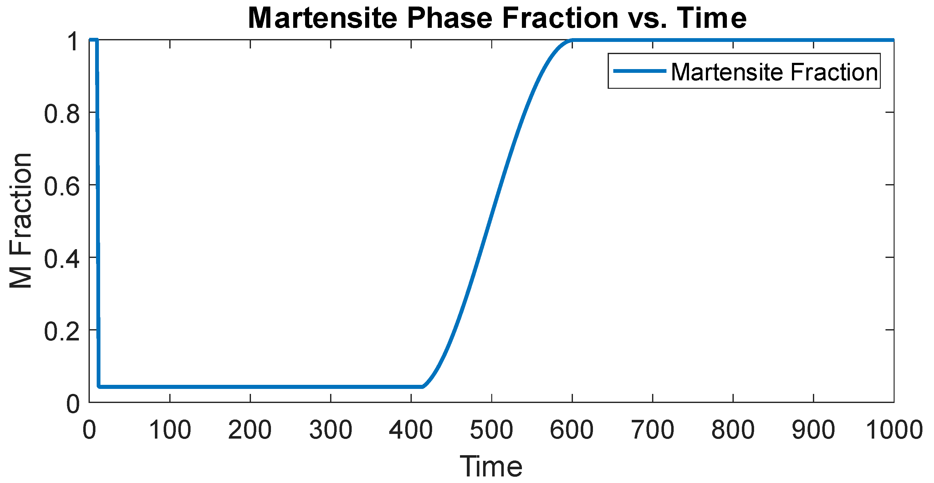
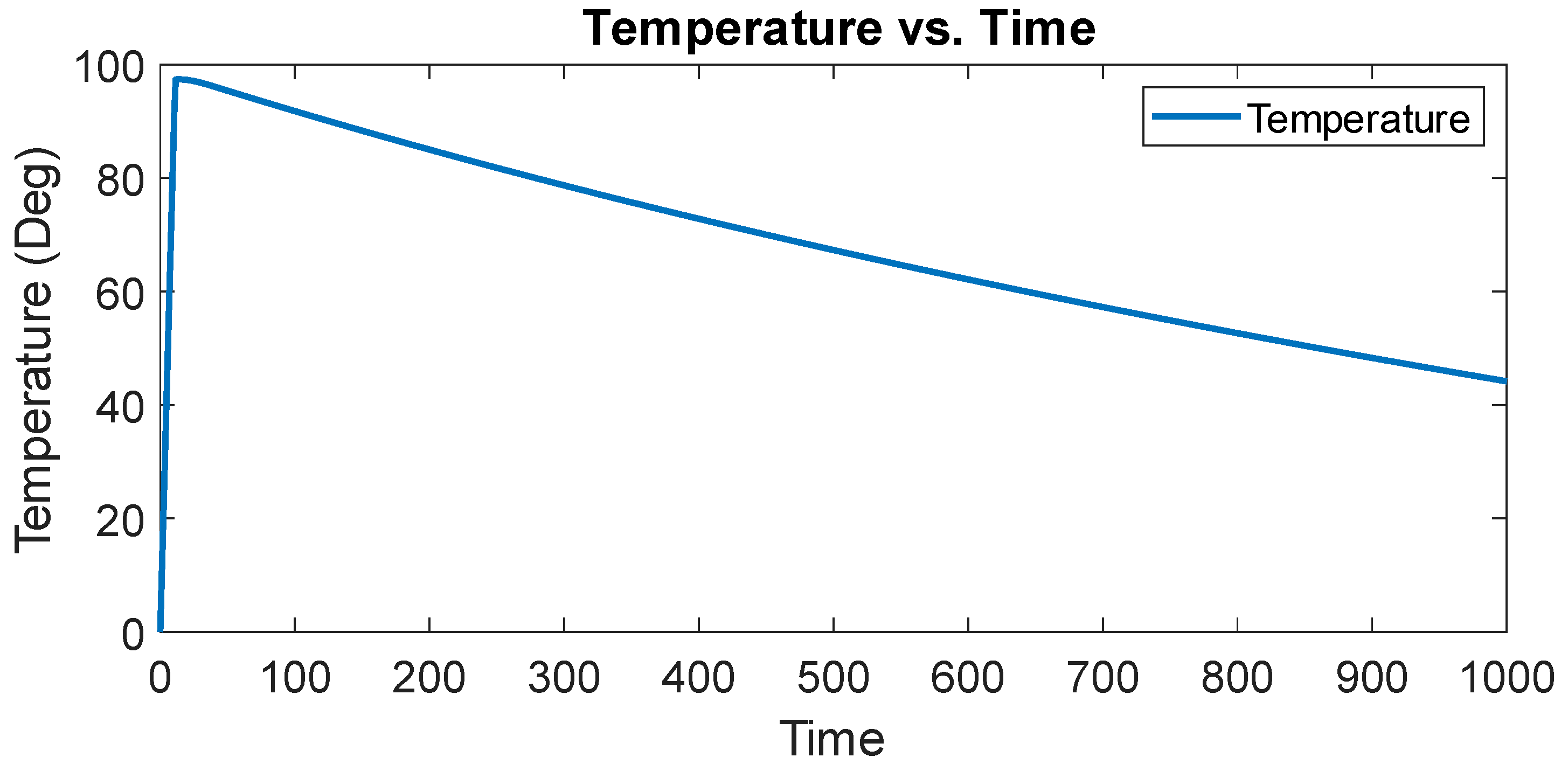
4.1. SMA Actuator Control

Table 1. List of parameters of SMA actuator [29].

Parameter	Value	Parameter	Value
Dm	28 GPa	cp	320 J/kg °C
Da	75 GPa	As	3.2 × 10−4 m2
As	88 °C	εmax	4%
Af	98 °C	d	0.015 m
Ms	72 °C	A	0.00103 m2
Mf	62 °C	E	5.51 MPa
M	5.27 × 10−3 kg/m	I2	5.26 × 10−8 m4
R	4.3 Ω/m	CM	10 MPa/°K
L	0.1 m	CA	10 MPa/°K
Θ	0.055 MPa/°C	T0	−100 °C
Aa	8.17 × 10−7 m2	rw	0.51 mm

lists the parameters used by the proposed SMA actuator.

Figure 8 shows the implementation of a PIDNN control model for the SMA actuator. It receives desired angle as input and uses the angle error and actual output to adjust the PID gain.

The relationship between the temperature and strain is captured as displayed in Figure 9, which is a hysteresis loop.

The desired deflection is a step signal with a width of 1200 s and value of $7^{°}$; the results are obtained as shown in Figure 10.

It can be seen from the test results that the PIDNN controller can track the reference. A 320 s delay is observed during the SMA actuator returning to its original shape. This is because only radiation takes effect in the cooling process in the space environment. The state convergence takes around 800 s, which is much longer than a conventional tendon-driven actuator. This is again because the overshoot also involves the cooling process of the SMA actuator, which is limited by the cooling method in the space environment. The performance can be improved by adjusting the offset of output layer of BPNN as shown in Figure 11, where the steady state error exists but it shows a higher bandwidth since the overshoot is reduced.

The temperature and martensite fraction are shown in Figure 12 and Figure 13. The delay in actuation time by forward phase transformation and the slow rate of de-actuation by reverse phase transformation are observed.

In addition to the single step signal, a sinusoidal signal is also sent to the control model. With a frequency of 1/450 rad/s, the initial simulation of the desired and actual deflection of the SMA actuator is shown in Figure 14 that the PIDNN controller can track the reference signal well after the first sinusoidal wave, particularly during the actuation stage. This implies that the BP neural network works as it tunes the PID parameter to reduce the error. However, Figure 14 shows lower tracking performance during the de-actuation stage when the controller instructs the actuator to return to its original shape due to the radiation-only cooling process in space as also discussed above and observed in Figure 10 and Figure 11. This observation indicates the necessity of implementing an active SMA cooling method and the corresponding control algorithm for improved actuation performance.

We conduct a series of simulation tests in Figure 15, Figure 16 and Figure 17 to determine the bandwidth of the actuator where the bandwidth of about 1/200 rad/s is observed. It is clear from Figure 15, Figure 16 and Figure 17 that the actuator can track the reference signal when its frequency is less than half of the actuator’s bandwidth which obeys the Nyquist–Shannon sampling theorem. Figure 17 shows the reference signal is about two-thirds of the actuator bandwidth. In this case, the actuator cannot respond to the signal well because the higher-frequency signal allows less time for the radiation-only cooling process of the SMA actuator. Overall, the control performance of the PIDNN has been confirmed by the results from these simulations.

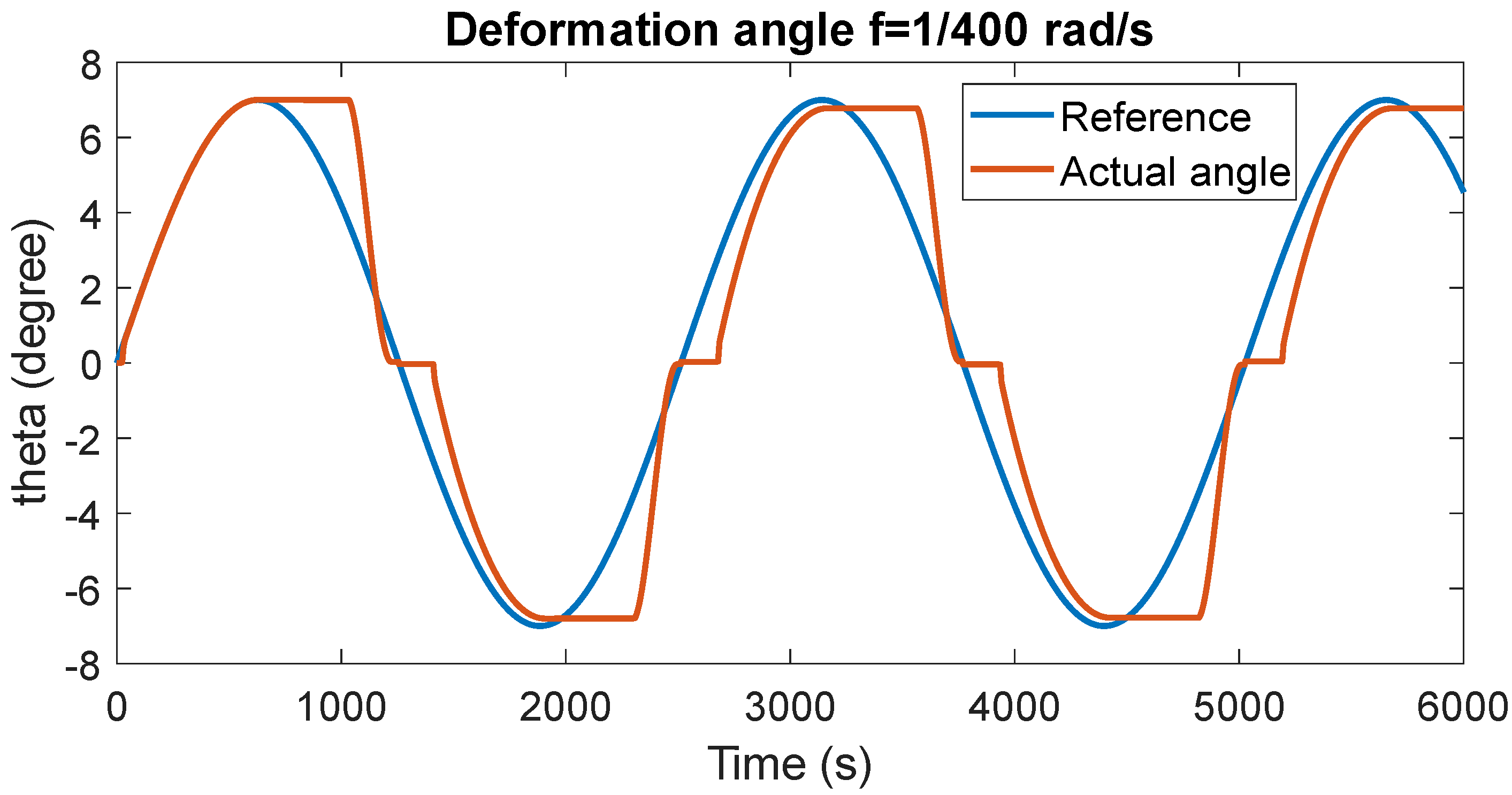
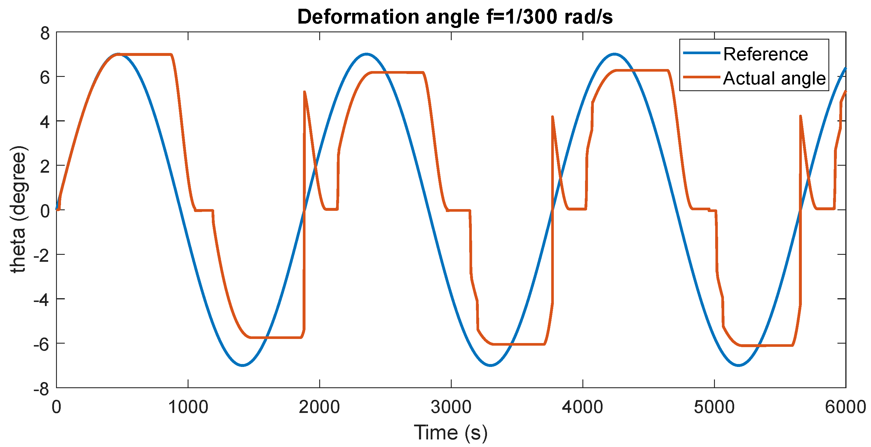
4.2. Attitude Control of Solar Sail

Table 2. List of Parameters of a Cubesat Solar Sail.

Parameter	Description	Value
ms	Total Mass	3 kg
I	Moment of Inertia	[0.3104 0.3104 0.5757] kg m2
Ls	Side Length	40 m
Asail	Total Sail Area	1600 m2
γ	Initial Roll Angle	0°
β	Initial Yaw Angle	0°
φ	Initial Pitch Angle	0°
Eo	CM/CP offset	0.25%
α	Incident angle of Sun	0°

lists the parameters of the solar sail design based on the 3U CubeSat platform. The moment of inertia of the spacecraft corresponds to those after the solar sail is deployed.

The proposed solar sail attitude control algorithm and the controller for the actuators form a cascade control loop with two controllers. Typically, a cascade controller aims to reject disturbance before its propagation; in this case the inner controller is designed to deal with the non-linearity of the SMA actuator.

Figure 18 shows the attitude control of the CubeSat solar sail, given the disturbance of CM/CP offset (0.25%). The result shows that the CubeSat solar sail can successfully perform a 45° maneuver in the pitch axis within 14 h. To reduce the overshoot, a large derivative gain is used; this will also help reduce the SMA forward transformation times in the further control. The control torque acting on the solar sail depends on the size of the solar sail and the Sun angle. The maximum torque generated during this simulation is 1.5 × 10⁻³ Nm with the sail size being 1600 m² when it faces the Sun directly in Figure 18. The maximum control torque for a 25 m², however, is about 6 × 10⁻⁵ Nm. The CM/CP offset disturbance caused by manufacturing error is relatively small compared with attitude control torque. However, the CM/CP offset still needs to be counteracted throughout the simulation that requires tiny sail deflection. After finishing the maneuver, the sail craft stops.

5. Discussion and Conclusions

A new solar sail attitude control concept was proposed, employing eight SMA bending actuators for attitude control; this sail craft allowed four quadrant sails to rotate or bend to change CM/CP offset with the maximum torque generated which is 1.5 × 10⁻³ Nm. This type of actuation mechanisms offers large control torque without compromising mass requirement. Mathematical model and quaternion-based PD control method were developed to verify such a configuration. Through a number of simulations, the configuration was shown to be controlled by the quaternion PD control, where external disturbance of the offset error was considered. We showed that our proposed approach could achieve the reasonable tracking performance up to 1/600 rad/s reference signal and effectively handle external disturbance of the offset error. This solar sail attitude control alternative is scalable and can be applied in solar sails with different sizes.

Cascade control of attitude using SMA actuator was simulated. The SMA actuator and attitude control method was shown to provide accurate attitude control in pitch axis for solar sail. It is able to rotate the spacecraft 45° in 14 h. It was noticed that the deflection bandwidth of the actuator significantly limited its ability of controlling sail craft attitude during de-actuation phases. In future works, we plan to further investigate the proposed approach with an active SMA cooling mechanism and corresponding control algorithm for improved performance in attitude control for solar sails.

References

1. Spencer, D.A.; Johnson, L.; Long, A.C. Solar sailing technology challenges. Aerosp. Sci. Technol. 2019, 93, 105276. [Google Scholar] [CrossRef]
2. Tsuda, Y.; Mori, O.; Funase, R.; Sawada, H.; Yamamoto, T.; Saiki, T.; Endo, T.; Yonekura, K.; Hoshino, H.; Kawaguchi, J.I. Achievement of IKAROS—Japanese deep space solar sail demonstration mission. Acta Astronaut. 2013, 82, 183–188. [Google Scholar] [CrossRef]
3. Song, Y.; Gong, S. Solar-sail trajectory design for multiple near-Earth asteroid exploration based on deep neural networks. Aerosp. Sci. Technol. 2019, 91, 28–40. [Google Scholar] [CrossRef] [Green Version]
4. Underwood, C.; Viquerat, A.; Schenk, M.; Taylor, B.; Massimiani, C.; Duke, R.; Stewart, B.; Fellowes, S.; Bridges, C.; Aglietti, G. InflateSail de-orbit flight demonstration results and follow-on drag-sail applications. Acta Astronaut. 2019, 162, 344–358. [Google Scholar] [CrossRef] [Green Version]
5. Perakis, N.; Schrenk, L.E.; Gutsmiedl, J.; Koop, A.; Losekamm, M.J. Project Dragonfly: A feasibility study of interstellar travel using laser-powered light sail propulsion. Acta Astronaut. 2016, 129, 316–324. [Google Scholar] [CrossRef]
6. Niccolai, L.; Caruso, A.; Quarta, A.A.; Mengali, G. Artificial collinear Lagrangian point maintenance with electric solar wind sail. IEEE Trans. Aerosp. Electron. Syst. 2020, 56, 4467–4477. [Google Scholar] [CrossRef]
7. Farrés, A.; Heiligers, J.; Miguel, N. Road Map to L4/L5 with a solar sail. Aerosp. Sci. Technol. 2019, 95, 105458. [Google Scholar] [CrossRef]
8. Mengali, G.; Quarta, A.A. Solar sail trajectories with piecewise-constant steering laws. Aerosp. Sci. Technol. 2009, 13, 431–441. [Google Scholar] [CrossRef]
9. Peloni, A.; Rao, A.V.; Ceriotti, M. Automated trajectory optimizer for solar sailing (atoss). Aerosp. Sci. Technol. 2018, 72, 465–475. [Google Scholar] [CrossRef] [Green Version]
10. Niccolai, L.; Quarta, A.A.; Mengali, G. Solar sail trajectory analysis with asymptotic expansion method. Aerosp. Sci. Technol. 2017, 68, 431–440. [Google Scholar] [CrossRef]
11. Pan, X.; Xu, M.; Santos, R. Trajectory optimization for solar sail in cislunar navigation constellation with minimal lightness number. Aerosp. Sci. Technol. 2017, 70, 559–567. [Google Scholar] [CrossRef]
12. Bassetto, M.; Quarta, A.A.; Mengali, G.; Cipolla, V. Trajectory Analysis of a Sun-Facing Solar Sail with Optical Degradation. J. Guid. Control Dyn. 2020, 43, 1727–1732. [Google Scholar] [CrossRef]
13. Caruso, A.; Niccolai, L.; Mengali, G.; Quarta, A.A. Electric sail trajectory correction in presence of environmental uncertainties. Aerosp. Sci. Technol. 2019, 94, 105395. [Google Scholar] [CrossRef]
14. Huo, M.; Mengali, G.; Quarta, A.A.; Qi, N. Electric sail trajectory design with Bezier curve-based shaping approach. Aerosp. Sci. Technol. 2019, 88, 126–135. [Google Scholar] [CrossRef]
15. Niccolai, L.; Quarta, A.A.; Mengali, G. Analytical solution of the optimal steering law for non-ideal solar sail. Aerosp. Sci. Technol. 2017, 62, 11–18. [Google Scholar] [CrossRef]
16. Wang, W.; Mengali, G.; Quarta, A.A.; Baoyin, H. Decentralized fault-tolerant control for multiple electric sail relative motion at artificial Lagrange points. Aerosp. Sci. Technol. 2020, 103, 105904. [Google Scholar] [CrossRef]
17. Liu, J.; Rong, S.; Shen, F.; Cui, N. Dynamics and control of a flexible solar sail. Math. Probl. Eng. 2014, 2014. [Google Scholar] [CrossRef] [Green Version]
18. Wie, B. Solar sail attitude control and dynamics, part 1. J. Guid. Control Dyn. 2004, 27, 526–535. [Google Scholar] [CrossRef]
19. Sperber, E.; Fu, B.; Eke, F. Large angle reorientation of a solar sail using gimballed mass control. J. Astronaut. Sci. 2016, 63, 103–123. [Google Scholar] [CrossRef]
20. Wie, B. Solar sail attitude control and dynamics, part two. J. Guid. Control Dyn. 2004, 27, 536–544. [Google Scholar] [CrossRef]
21. Fu, B.; Sperber, E.; Eke, F. Solar sail technology—A state of the art review. Prog. Aerosp. Sci. 2016, 86, 1–19. [Google Scholar] [CrossRef]
22. Niccolai, L.; Mengali, G.; Quarta, A.A.; Caruso, A. Feedback control law of solar sail with variable surface reflectivity at Sun-Earth collinear equilibrium points. Aerosp. Sci. Technol. 2020, 106, 106144. [Google Scholar] [CrossRef]
23. Bianchi, C.; Niccolai, L.; Mengali, G.; Quarta, A.A. Collinear artificial equilibrium point maintenance with a wrinkled solar sail. Aerosp. Sci. Technol. 2021, 119, 107150. [Google Scholar] [CrossRef]
24. Qu, Q.; Xu, M.; Luo, T. Design concept for In-Drag Sail with individually controllable elements. Aerosp. Sci. Technol. 2019, 89, 382–391. [Google Scholar] [CrossRef]
25. Mavroidis, C. Development of advanced actuators using shape memory alloys and electrorheological fluids. J. Res. Nondestruct. Eval. 2002, 14, 1–32. [Google Scholar] [CrossRef]
26. Bovesecchi, G.; Corasaniti, S.; Costanza, G.; Tata, M.E. A novel self-deployable solar sail system activated by shape memory alloys. Aerospace 2019, 6, 78. [Google Scholar] [CrossRef] [Green Version]
27. Elahinia, M.H.; Ashrafiuon, H. Nonlinear control of a shape memory alloy actuated manipulator. J. Vib. Acoust. 2002, 124, 566–575. [Google Scholar] [CrossRef]
28. Elahinia, M.; Esfahani, E.T.; Wang, S. Control of sma systems: Review of the state of the art. Shape Mem. Alloy. Manuf. Prop. Appl. 2011, 381–392. [Google Scholar]
29. Kannan, S. Modeling and Control of Shape Memory Alloy Actuator. Ph.D. Thesis, Ecole Nationale Supérieure D’arts et Métiers-ENSAM, Paris, France, 2011. [Google Scholar]
30. Yang, K.; Chenglin, G. Variable Structure Controller Of Novel Embedded Sma Actuators. IU-J. Electr. Electron. Eng. 2011, 5, 1255–1263. [Google Scholar]
31. Razov, A.; Cherniavsky, A. Applications of shape memory alloys in space engineering: Past and future. In Proceedings of the 8th European Space Mechanisms and Tribology Symposium, Toulouse, France, 29 September–1 October 1999; p. 141. [Google Scholar]
32. Schetky, L.M. Shape memory alloy applications in space systems. Mater. Des. 1991, 12, 29–32. [Google Scholar] [CrossRef]
Figure 1. SMA Wire Block Diagram.
Aerospace 08 00372 g001
Figure 2. (a) Bending SMA actuator; (b) actuator configuration [30].
Aerospace 08 00372 g002
Figure 3. The integration of the actuators and the solar sail.
Aerospace 08 00372 g003
Figure 4. Actuator block diagram.
Aerospace 08 00372 g004
Figure 5. Deployed Solar Sail with Rotated Membranes.
Aerospace 08 00372 g005
Figure 6. Structure of BPNN for Adaptive PID Control.
Aerospace 08 00372 g006
Figure 7. Solar Sail Attitude Control Loop.
Aerospace 08 00372 g007
Figure 8. PIDNN control for SMA actuator.
Aerospace 08 00372 g008
Figure 9. SMA model validation.
Aerospace 08 00372 g009
Figure 10. SMA Control Response to Step input.
Aerospace 08 00372 g010
Figure 11. SMA control response with small offset to step input.
Aerospace 08 00372 g011aAerospace 08 00372 g011b
Figure 12. Martensite fraction change to step input using PIDNN.
Aerospace 08 00372 g012
Figure 13. Temperature change to step input using PIDNN.
Aerospace 08 00372 g013
Figure 14. SMA actuator response to positive sinusoidal wave.
Aerospace 08 00372 g014
Figure 15. SMA control response to sin input (f = 1/600 rad/s).
Aerospace 08 00372 g015
Figure 16. SMA control response to sin input (f = 1/400 rad/s).
Aerospace 08 00372 g016
Figure 17. SMA control response to sin input (f = 1/300 rad/s).
Aerospace 08 00372 g017
Figure 18. Attitude control of a CubeSat solar sail with the sail size of 1600 m2.
Aerospace 08 00372 g018aAerospace 08 00372 g018b