Article

Free-Vertex Tetrahedral Finite-Element Representation and Its Use for Estimating Density Distribution of Irregularly-Shaped Asteroids

1
Key Laboratory of Space Utilization, Technology and Engineering Center for Space Utilization, Chinese Academy of Sciences, Beijing 100094, China
2
University of Chinese Academy of Sciences, Beijing 100049, China
3
School of Aeronautical Science and Engineering, Beihang University, Beijing 100091, China
*
Author to whom correspondence should be addressed.
Aerospace 2021, 8(12), 371; https://doi.org/10.3390/aerospace8120371
Submission received: 31 August 2021 / Revised: 19 November 2021 / Accepted: 28 November 2021 / Published: 30 November 2021
(This article belongs to the Special Issue Spacecraft Dynamics and Control)

Abstract

:
In this article, we present a free-vertex tetrahedral finite-element representation of irregularly shaped small bodies, which provides an alternative solution for estimating asteroid density distribution. We derived the transformations between gravitational potentials expressed by the free-vertex tetrahedral finite elements and the spherical harmonic functions. Inversely, the density of each free-vertex tetrahedral finite element can be estimated via the least-squares method, assuming a spherical harmonic gravitational function is present. The proposed solution is illustrated by modeling gravitational potential and estimating the density distribution of the simulated asteroid 216 Kleopatra.

1. Introduction

Asteroids, as remnants of the early stages of planet formation, have the potential to advance knowledge about the origin of the solar system. Knowledge of the internal structure of asteroids is of great significance for understanding the origin, evolution, and current state of asteroids [1]. Although the interior cannot be observed directly, other information can be used to assist in gaining an up-to-date understanding. For example, in the study of the internal structure of planetary moons, Durante et al. [2] used flyby data to determine the gravitational field to degree and order 5, which improved the estimated value of tidal Love number k2 and determined that Titan has a strongly differentiated interior. Cappuccio et al. [3] used Ganymede’s gravity field and tide response, determined by Doppler and range data from a 500 km circular orbit in the 3GM experiment simulation, to provide critical information for accurately modeling Ganymede’s internal structure. However, the size of most asteroids is smaller than these moons, and we have less prior knowledge of the internal structure, although many asteroid exploration missions have measured their gravity fields [4,5,6]. Additionally, many asteroids are considered to be rubble pile asteroids, and their internal composition and structure may be unconstrained [7]. Therefore, if it is possible to estimate the internal structure of asteroids with a tiny amount of information about them (only the gravity field and shape data are available); this will be of great help for research on asteroids. What factors are related to the estimation of the internal structure of asteroids? Since it is difficult to directly detect the internal structure, we can indirectly obtain the distribution of the internal structure from the density and gravity field information of asteroids. Density is indeed a fundamental property for understanding their composition and internal structure [1], which means that the density of asteroids may reflect their internal composition. Otherwise, the asteroid gravity field implies information about the density and internal structure of asteroids. An accurate gravity field will help asteroid exploration missions, such as in the design of frozen orbits [8]. Therefore, this paper aims to establish a new gravity field model of asteroids that can be used to estimate their density distribution. The performance of density estimation is investigated in two cases: (1) the internal structure with no prior information; and (2) the internal structure with prior information.
There are three fundamental solutions for modeling the gravitational field of an asteroid (or a comet): the spherical harmonic function [9], the polyhedron model [10], and the mascon method [11]. As each of these solutions has its pros and cons, a series of improved models have been proposed to either increase the computational efficiency or improve the fineness of computing irregularly shaped asteroid gravitation [12,13,14,15,16]. Among these improved models, the tetrahedral finite-element method (FEM) [17,18] attracts the most attention since it combines the advantages of the polyhedron (excellent asteroid irregular surface representation) and the mascon (non-uniform density distribution representation) approaches. The basic idea of the tetrahedral FEM is to use tetrahedral elements to fill up an asteroid’s spatial shape, and the faces of the outer-layer elements approximate the asteroid’s irregular surface. The volume of each tetrahedral element is determined by the specific meshing method with either coarse meshes or fine meshes. In the literature, there are two representative types of finite element meshes in the tetrahedral FEM, which are depicted in Figure 1: centroid-vertex meshes and free-vertex meshes. The former was first proposed by Scheeres et al. [16], in which at least one of the vertexes of all finite elements is constrained at the center of mass of the asteroid. However, this approach cannot directly express the internal density distribution of asteroids, such as the rubble piles model [19,20], the elongated bi-lobed model (4179 Toutatis [21] and comet 67P/Churyumov–Gerasimenko [22]) and the hypothetical model (the planar cut model, the surface layer model, the one core model, the two-core model, and the torus model, proposed by Takahashi et al. [23]). In contrast, the free-vertex meshes can remove the constraint assumed in the centroid-vertex meshes, providing a more flexible solution for generating tetrahedral finite elements. Therefore, this article focuses on presenting the free-vertex tetrahedral finite-element representation and its use for estimating the density distribution of irregularly shaped asteroids, which may be helpful for obtaining the internal structure of these small bodies.
The concept of the tetrahedral FEM for asteroid shape representation can be traced independently back to the concepts of the mascon method and the polyhedron model. To overcome the shortcomings of the mascon method in describing the shapes of asteroids, Pearl and Hitt proposed the tetrahedral FEM and higher-order polyhedral FEM meshes (which are called polyhedral-dual meshes, different from the polyhedral model) [24], and they found that the number of mascons derived from the FEM meshes can be reduced by 90% compared with the uniformly distributed mascons [14]. Pearl et al. [25] then compared the mascons derived from different FEM meshes with the polyhedron model and showed that the FEM-based mascons are more accurate for computing asteroid gravitation than the polyhedron model in some specific regions, such as a thin region that hugs the surface of the asteroid. Moreover, Rathinam et al. [26] suggested that the mascons based on the octree approach (a mesh generation method of FEM) are more computationally efficient than the polyhedron model. On the other hand, the tetrahedral FEM can also be obtained by improving the polyhedral model, which assumes a constant density distribution. Park et al. [27] used finite element spheres and finite element cubes to approximate the shape of asteroids, but there are gaps between the elements, and the surface is not smooth. Recently, Yu et al. [18] proposed an approach of computing the gravitational potentials of the binary asteroids using the free-vertex tetrahedral finite element and showed the effectiveness of the tetrahedral FEM. Yin et al. [17] found that the free-vertex tetrahedral finite element model can fit the structure of small bodies better than the polyhedron model.
The tetrahedral FEM with the variable meshing method is more suitable for the study of the asteroid density distribution than the polyhedron model and the mascon method, as it provides representations of the non-uniform density distribution of an asteroid with finer meshes. However, it is difficult to obtain the internal density distribution of the asteroid even if we can detect the gravity field and shape of the asteroid. A solution for estimating the density distribution of asteroids was proposed by Scheeres et al. [16]; the method uses the relationship between the spherical harmonic coefficients and the tetrahedral model to determine the density of each centroid-vertex tetrahedron by applying a least-squares method. Then, Park et al. [27] applied an alternative method using navigation measurements such as station-to-spacecraft tracking to estimate density distribution. However, the asteroid density distribution is quite unlikely to be accurately approximated by the centroid-vertex tetrahedral elements. Takahashi et al. [23,28] and Ledbetter et al. [29] divided the centroid-vertex tetrahedron element into layers, but the accuracy of density distribution estimation is still limited.
In summary, the motivation of this study is to investigate the use of the free-vertex tetrahedral FEM for representing an asteroid’s spatial shape and density distribution. It is deemed a follow-up advancement of density distribution estimation using the strip-shaped elements observed in the centroid-vertex tetrahedral FEM [16]. In Section 2, the free-vertex tetrahedral finite element gravitation model is introduced. In Section 3, we derive the transformations between gravitational potentials expressed by the free-vertex tetrahedral finite elements and the spherical harmonic functions, and a least-squares method is used to estimate the density of each free-vertex tetrahedral finite element. In Section 4, we consider the asteroid 216 Kleopatra [30] as an example to demonstrate the free-vertex tetrahedral FEM. Conclusions are presented in Section 5.

2. Free-Vertex Tetrahedral Finite Element Gravitation Model

The gravitational potential and force caused by each free-vertex tetrahedral finite element (which can also be called a tetrahedron) can be calculated by applying the polyhedron method [10], and then the values of each potential and force are added up to obtain the gravitational potential U p o l y t e t r a and the gravitational force U p o l y t e t r a for a specific asteroid, which are given below.
U p o l y t e t r a = 1 2 G i = 1 n ρ i e e d g e s r e i · E e i · r e i · L e i f f a c e s r f i · F f i · r f i · ω f i
U p o l y t e t r a = G i = 1 n ρ i e e d g e s E e i · r e i · L e i f f a c e s F f i · r f i · ω f i ,
where G is the universal gravitational constant, i is the serial number of the tetrahedral elements, ρ i is the density of the numbered tetrahedral element, e represents the edge of the tetrahedron, and 
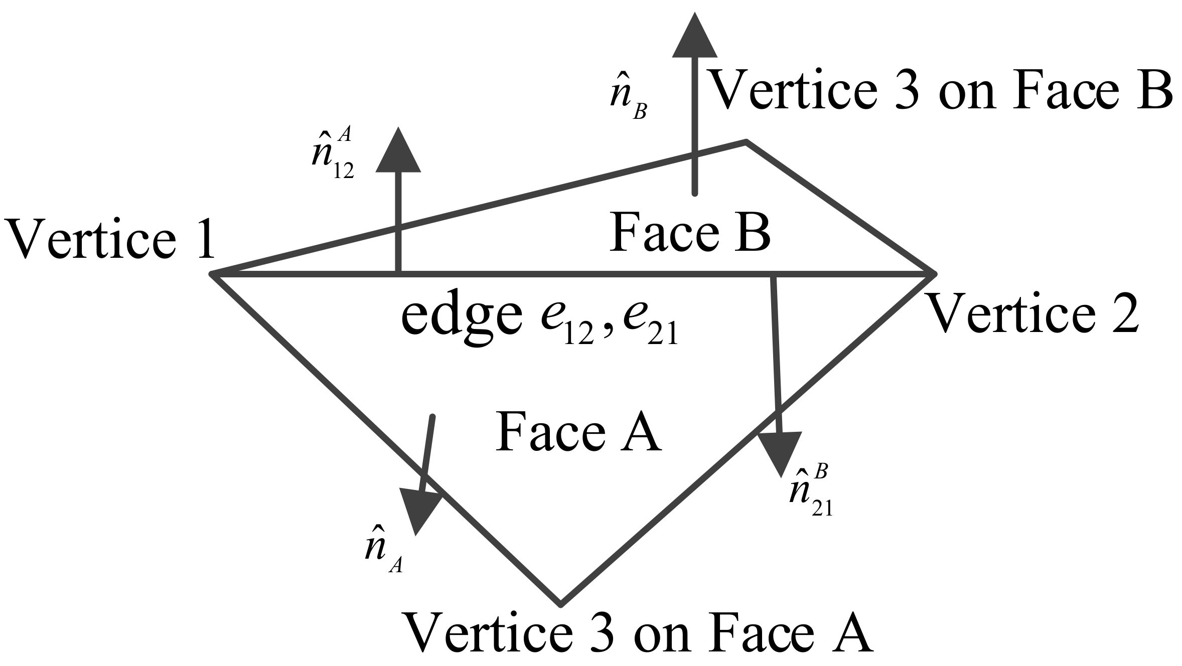
f represents the triangular face by three vertices of the tetrahedron.
F f i = n ^ f n ^ f E e i = n ^ A n ^ e A + n ^ B n ^ e B L e i = e 1 r d s = P l P j 1 r d s = ln r l + r j + e l j r l + r j e l j ω f i = t r i a n g l e Δ z r 3 d S = 2 · arctan r l · r j × r k r l r j r k + r l r j · r k + r j r k · r l + r k r l · r j ,
where F f i is the dyad related to the triangular face, E e i is the dyad related to the edge, L e i is the dimensionless factor of each edge, ω f i is the dimensionless factor of each face, n ^ f represents the outward-pointing surface normal direction vector of the face, and n ^ e f is the normal direction vector of the edge of the face lying in the face plane, which is orthogonal to both the face normal vector and the along-the-edge vector, and points outward. A and B are the symbols of the two faces that have common edges, respectively. r l , r j and r k represent the vectors from the field point to the three vertices of the triangle surface, respectively, and r l , r j , and r k are the modulus of the corresponding vectors. The edges and faces, as well as the normal direction vectors, are shown in Figure 2.
The free-vertex tetrahedral finite element model is obtained by mesh generation methods [31]. The structured mesh is composed of horizontal and vertical lines that cross orthogonally at intersections called nodes. Generally, the structured mesh generation process is best achieved by discretizing the physical domain defined by the square or rectangular boundary; thus, it is mainly suitable for simple geometric shapes. In unstructured meshes, the nodes used to discretize the two-dimensional physical domain change from being ordered orthogonally in the structured mesh to seemingly randomly placed. These nodes are connected to other nodes via triangular or quadrilaterally shaped subdomains or elements. In the three-dimensional physical domain, the most common types of elements are tetrahedrons and hexahedrons. The generation of unstructured meshes requires more thought and effort than structured meshes. In general, one puts more nodes (or elements) near surfaces and in regions where activity (or steep gradients) is likely to occur. Therefore, the unstructured mesh is a better choice for irregularly shaped asteroids. The unstructured mesh can be generated by the octree algorithm [32], the Delaunay algorithm [31] or the advancing front algorithm [33]. The Octree algorithm uses a cube to cover the entire shape area that needs to be meshed, and then continuously subdivides the cube according to the requirements of the mesh size. The advancing front algorithm generates tetrahedral elements from the boundary of the meshed area and continues to advance to the center until the entire area is covered by tetrahedral elements. The Delaunay algorithm requires the tetrahedron to satisfy the Delaunay criterion [31]; that is, there are no other points in the circumscribed ball of each tetrahedron, except for its own four vertices. A significant advantage of the Delaunay algorithm is that it can make the minimum angle of each tetrahedron element in the mesh system constituted by a given point set as large as possible, allowing us to obtain tetrahedron elements with as high a quality as possible.
The asteroid 216 Kleopatra is taken to generate the free-vertex tetrahedral meshes as an example. As shown in Figure 3, the shape model of Kleopatra is modeled as the polyhedron model and the free-vertex tetrahedral FEMs. The meshes of the tetrahedral FEMs are generated by the Delaunay triangulation algorithm [31] with different maximum element growth rates (the difference between the sizes of two adjacent elements).
Since we generate the free-vertex tetrahedral FEMs, if we obtain the prior information about the density distribution, we can calculate the gravitational field of the asteroid. Although the meshes of these models are different, the gravity field calculated by each FEM is valid if the density distribution of the corresponding mesh can be obtained. This also shows that the meshes of the free-vertex tetrahedral FEMs are not restricted by the internal structures of the asteroid. On the contrary, if the internal structures are known, the divided tetrahedral finite elements can be combined into the corresponding structures, which is also the reason that we propose the free-vertex tetrahedral FEM.

3. Transformation for Gravity Field Expressions

3.1. Transformation from Free-Vertex Tetrahedral FEM to Spherical Harmonics with Simplex Integral

The spherical harmonic expansion of the gravitational potential [34] is expressed by:
U s p h e r i c a l = G M A r n = 0 N m = 0 n r e r n P n m sin φ C n m cos m λ + S n m sin m λ ,
where r is the distance of the field point to the center of the expansion, and λ and φ are the longitude and latitude of the field point, respectively. P n m sin φ is the associated Legendre polynomial; r e is the radius of the reference sphere, which represents the convergence range of the series; M A is the total mass of the asteroid; n and m are the degree and order of the expansion, respectively; and C n m and S n m are the spherical harmonic coefficients that are specified up to degree N. The coefficient C 00 = 1 and the total number of gravitational coefficients is N + 1 2 , with 2 n + 1 coefficients at each degree n.
The fully normalized harmonic coefficients, C ¯ n , m and S ¯ n , m , can be calculated analytically by approximating the extended body with a swarm of points [35]:
C ¯ n , m S ¯ n , m = i point masses c ¯ n , m x i , y i , z i s ¯ n , m x i , y i , z i M i ,
where M i is the point’s mass, and c ¯ n , m and s ¯ n , m are integrands of the point’s normalized spherical harmonic coefficients. x , y , z are the coordinates that represent the point.
Then, the point is replaced by a tetrahedron. The density ρ i of each tetrahedron is assumed to be constant, and the coefficients C ¯ n , m and S ¯ n , m can be written as the following integral form:
C ¯ n , m S ¯ n , m = extended body c ¯ n , m s ¯ n , m d m = extended body ρ i c ¯ n , m s ¯ n , m d x d y d z .
The recurrent relationships for integrands c ¯ n , m and s ¯ n , m proposed by Werner et al. [35] are as follows:
sectorial : n = 0 : c ¯ 0 , 0 s ¯ 0 , 0 = 1 M 1 0 n = 1 : c ¯ 1 , 1 s ¯ 1 , 1 = 1 3 M x x r e r e y y r e r e n > 1 : c ¯ n , n s ¯ n , n = 2 n 1 2 n 2 n + 1 x x r e r e y y r e r e y y r e r e x x r e r e c n 1 , n 1 s n 1 , n 1 vertical : c ¯ n , m s ¯ n , m = 2 n 1 2 n 1 2 n + 1 n + m n m z r e × c ¯ n 1 , m s ¯ n 1 , m 2 n 3 n + m 1 n m 1 2 n + 1 n + m n m r r e 2 c ¯ n 2 , m s ¯ n 2 , m subdiagonal : c ¯ n , n 1 s ¯ n , n 1 = 2 n 1 2 n + 1 z r e c ¯ n 1 , n 1 s ¯ n 1 , n 1 ,
where r e is the radius of the reference sphere, and r = x 2 + y 2 + z 2 .
Although the recurrence relationships of spherical harmonic coefficients are given, they cannot be applied directly to calculate c ¯ n , m and s ¯ n , m of the free-vertex tetrahedral finite elements proposed in this article as the coordinates x , y , z cannot be obtained directly for a tetrahedron. Furthermore, as the asteroid model used in Werner et al. [35] and Scheeres et al. [16] is the centroid-vertex tetrahedral finite element, we cannot simply refer to their calculation results of the spherical harmonic coefficients. Therefore, we re-derived the calculation of spherical harmonic coefficients based on the free-vertex tetrahedral FEM in this study. The coordinates x , y , z of the given free-vertex tetrahedral elements P 0 P 1 P 2 P 3 are denoted as x 0 , y 0 , z 0 , x 1 , y 1 , z 1 , x 2 , y 2 , z 2 and x 3 , y 3 , z 3 , which are different from those defined in [35]: 0 , 0 , 0 , x 1 , y 1 , z 1 , x 2 , y 2 , z 2 and x 3 , y 3 , z 3 . In order to solve Equation (6), variable conversion is needed, and the coordinates x , y , z are expressed with standard simplex coordinates u 0 , u 1 , u 2 , u 3 by the relation [36]:
1 x y z = 1 1 1 1 x 0 x 1 x 2 x 3 y 0 y 1 y 2 y 3 z 0 z 1 z 2 z 3 u 0 u 1 u 2 u 3 .
Here, the simplex refers to the free-vertex tetrahedral finite element, and the standard simplex is defined with coordinates u 0 , u 1 , u 2 , u 3 : 0 , 0 , 0 , 1 , 0 , 0 , 0 , 1 , 0 , 0 , 0 , 1 .
The expansion of Equation (8) is:
1 = u 0 + u 1 + u 2 + u 3 x u 0 , u 1 , u 2 , u 3 = x 1 u 1 + x 2 u 2 + x 3 u 3 + x 0 u 0 y u 0 , u 1 , u 2 , u 3 = y 1 u 1 + y 2 u 2 + y 3 u 3 + y 0 u 0 z u 0 , u 1 , u 2 , u 3 = z 1 u 1 + z 2 u 2 + z 3 u 3 + z 0 u 0 .
We use Equation (9) to replace x , y and z in Equation (7). The integrands c ¯ n , m and s ¯ n , m can be represented as follows:
c ¯ n , m x , y , z s ¯ n , m x , y , z c ¯ n , m u 0 , u 1 , u 2 , u 3 s ¯ n , m u 0 , u 1 , u 2 , u 3 = i 0 + i 1 + i 2 + i 3 = n α ¯ i 0 , i 1 , i 2 , i 3 β ¯ i 0 , i 1 , i 2 , i 3 u 0 i 0 u 1 i 1 u 2 i 2 u 3 i 3 .
Here, α ¯ h , j , k , l and β ¯ h , j , k , l are the tetranomial coefficients of coordinates u 0 , u 1 , u 2 , and u 3 . We provide examples of these in Appendix A.
Then, Equation (6) can be rewritten as follows:
C ¯ n , m S ¯ n , m = extended body c ¯ n , m s ¯ n , m d m = simplices ρ i det J i 0 + i 1 + i 2 + i 3 = n α ¯ i 0 , i 1 , i 2 , i 3 β ¯ i 0 , i 1 , i 2 , i 3 × standard simplex 1 = u 0 + u 1 + u 2 + u 3 u 0 i 0 u 1 i 1 u 2 i 2 u 3 i 3 d u 1 d u 2 d u 3 .
Here, the matrix J is the Jacobian matrix.
J x , y , z u 1 , u 2 , u 3 = x u 1 x u 2 x u 3 y u 1 y u 2 y u 3 z u 1 z u 2 z u 3 det J = x 1 x 0 x 2 x 0 x 3 x 0 y 1 y 0 y 2 y 0 y 3 y 0 z 1 z 0 z 2 z 0 z 3 z 0 = 1 x 0 y 0 z 0 1 x 1 y 1 z 1 1 x 2 y 2 z 2 1 x 3 y 3 z 3 .
Since the tetrahedral simplex integral is:
simplex 1 = u 0 + u 1 + u 2 + u 3 u 0 i 0 u 1 i 1 u 2 i 2 u 3 i 3 d u 1 d u 2 d u 3 = i 0 ! i 1 ! i 2 ! i 3 ! i 0 + i 1 + i 2 + i 3 + 3 ! ,
the expression of the spherical harmonic coefficients for the free-vertex tetrahedral finite element model is:
C ¯ n m S ¯ n m = simplics ρ i det J n + 3 ! i 0 + i 1 + i 2 + i 3 = n i 0 ! i 1 ! i 2 ! i 3 ! α ¯ i 0 , i 1 , i 2 , i 3 β ¯ i 0 , i 1 , i 2 , i 3 .
The integration of the simplex in Equation (13) is shown in Appendix B. In the process of analytically calculating simplex integrals, the tetranomial i 0 ! i 1 ! i 2 ! i 3 ! becomes increasingly complex as the degree of the spherical harmonic coefficients grows, and the dimensions of tetranomial coefficients become enormous due to the recurrent relationships in Equation (7), which requires large amounts of computing resources. In order to save computation time, the analytical solution can be approximated by numerical integration methods in finite element analysis [37], such as the Hammer integral [38,39]. This study used the Hammer integral to simplify calculations for the research. The details of the Hammer integral are shown in Appendix C.

3.2. Inverse Transformation from Spherical Harmonics to Free-Vertex Tetrahedral FEM with the Least-Squares Method

From Equation (14), an inverse transformation can be used to obtain the density of each free-vertex tetrahedron. The least-squares method proposed by Scheeres et al. [16] was used to evaluate the density distribution of the asteroid.
To estimate the density, the serial numbers of tetrahedrons and vertex coordinates were obtained. The usual form of the spherical harmonic gravitational potential is shown in Equation (4), and the potential needs to be rewritten by the tetrahedral finite element model:
U s p h e t e t r a = i p G V i ρ i r n = 0 N m = 0 n r e r n P ¯ n m sin θ C ¯ n m i cos m λ + S ¯ n m i sin m λ ,
where i is the index of the tetrahedron, p is the number of tetrahedrons, N is the degree of the highest calculated spherical harmonic coefficient, and C ¯ n m i and S ¯ n m i are the normalized spherical harmonic coefficients of the corresponding tetrahedron. Since the volume of the tetrahedron V i can be calculated from the geometric shape, due to the constant density hypothesis for each tetrahedron, the only unknown in the gravitational potential is the density ρ i .
The expression of the gravitational potential is different from the usual spherical harmonic gravitational potential. The usual form of Equation (4) is necessary to calculate the spherical harmonic coefficients of the whole asteroid and to consider the total mass of the asteroid, while in the free-vertex tetrahedral FEM, it is necessary to calculate the spherical harmonic coefficients corresponding to each tetrahedron separately, and then the potential of each tetrahedron is summed. Therefore, M refers to the mass of the tetrahedron in Equation (7).
Ideally, for the same asteroid, the gravitational potentials calculated by different models at the same location should be the same. For the inverse transformation, a least-squares method is used.
The loss function of the general least-squares method is given as:
J X ^ = Z H X ^ T Z H X ^ = min .
Here, X is the state vector, and the density ρ i is the element of the vector. X ^ is the estimation of the state vector. Z is the measurement vector, and H is the measurement matrix. In this study, the measurement is the real gravitational potential of the asteroid U s p h e r i c a l in Equation (4), and the calculated measurement H X ^ is the gravitational potential U s p h e t e t r a in Equation (15).
In order to minimize the function of the above equation, it is necessary to satisfy:
J X X = X ^ = 2 H T Z H X ^ .
Therefore, under the ideal situation, the estimated state vector X ^ can be expressed as:
X ^ = H T H 1 H T Z .
We can find that:
H = V i M C ¯ 10 1 V i M C ¯ 10 2 V i M C ¯ 10 p V i M C ¯ 11 i V i M C ¯ 11 2 V i M C ¯ 11 p V i M S ¯ 11 i V i M S ¯ 11 2 V i M S ¯ 11 p
Then, we can use the spherical harmonic coefficients to express Equation (18) and simplify the estimated solution as:
ρ = V i M C ~ n m i T V i M C ~ n m i 1 V i M C ~ n m i T C ~ n m ,
where ρ is the density vector, V i is the volume of the tetrahedron, M is the mass of the asteroid, and C ~ n m is a vector representation of the spherical harmonic coefficients: C ~ n m = C ¯ 10 , C ¯ 11 , S ¯ 11 , C ¯ 20 , C ¯ 21 , S ¯ 21 , , C ¯ N N , S ¯ N N .
If we measure the spherical harmonic coefficients of the asteroid, we can use weighted least-squares to calculate the state, which can be expressed as:
ρ = V i M C ~ n m i T W C ~ V i M C ~ n m i 1 V i M C ~ n m i T W C ~ C ~ n m ,
where W C ~ is the covariance matrix of the measured true spherical harmonic coefficients.
Then, we can use K and y to denote the matrixes:
K = V i M C ~ n m i T W C ~ V i M C ~ n m i y = V i M C ~ n m i T W C ~ C ~ n m .
Equation (21) can be abbreviated as:
ρ = K 1 y .
The dimension of ρ is p × 1 , and the dimension of C ~ n m is N + 1 2 1 × 1 . If the number of tetrahedrons is equal to ( N + 1 ) 2 1 , K is an invertible matrix, and there is a unique solution. If the number of constraints (tetrahedrons) is greater than the number of unknowns (the density of each tetrahedron), which is an overdetermined problem, the normal matrix is invertible, and the density of each tetrahedron can be obtained. When the number of tetrahedrons exceeds ( N + 1 ) 2 1 , the number of equations is less than the number of unknowns. If the normal matrix is not invertible and the system is under-determined, then the density cannot be solved by normal methods. In order to solve both cases at the same time, singular value decomposition (SVD) was used to solve Equation [16].
The singular value decomposition was performed by [40]:
K = U S V T ,
where U is an l × m orthogonal matrix and V is an m × m orthonormal matrix. Matrix S is an m × m diagonal matrix containing all the solved singular values, but if the ratio of the largest singular value to the smallest singular value is more than 10 16 , the condition number of the entire matrix will be abnormally large, which will cause the original problem to be poorly conditioned. Thus, the equation solution is very sensitive to disturbances. We selected condition number 10 13 to obtain an appropriate S ~ 1 .
The final solution of the least-squares method is:
ρ = V S ~ 1 U T y .
From this derivation process, it can be found that the accuracy of the density estimation depends on the number of tetrahedrons and the degree and order of spherical harmonic coefficients.

4. Density Distribution Estimation

In this section, a simulation in 216 Kleopatra is presented to verify the effectiveness of the free-vertex tetrahedral FEM for density distribution estimation. The mass of the asteroid 216 Kleopatra is 4.64 × 10 18 kg , and the reference radius of Kleopatra is 112 km. The coarse mesh that consists of 1467 tetrahedrons shown in Figure 3c was used. The volume of Kleopatra calculated by the proposed tetrahedral FEM is 6.8144 × 10 5 km 3 ; thus, its bulk density (the mass to volume ratio of Kleopatra) is 6.809 g / cm 3 . In these simulations, tetrahedrons can be used alone or assembled into polyhedrons. Then, we assigned densities to each tetrahedron (or polyhedron) to compute the “true” gravity potential, and the coefficients of the spherical harmonic function can be obtained from Equation (14). Then, the least-squares method was employed on the same shape discretization to verify that we recovered the proper densities for each tetrahedron (or polyhedron). Since the true gravitational field was fully known in our tests, the covariance matrix W C ~ became an identity matrix.

4.1. Density Distribution Estimation for Each Tetrahedron

We first estimated the density distribution when each tetrahedron acts as an independent unit of the free-vertex tetrahedral finite-element model. This indicates that the densities for elements of a mass distribution are estimated without prior information on the geometry of the distribution. This is of great significance for asteroid exploration missions. At the early stage of these missions, we do not particularly understand the internal structure of the target asteroid. If we can use shape information and the spherical harmonic gravitational field information in the mission to detect the asteroid, we can find out whether the interior of the asteroid is uniform, or whether there are density mutations or hollows.
Since the number of tetrahedrons is 1467, which is larger than the dimensions of the vector of the spherical harmonic coefficients ( n 37 ), the problem of estimating the density distribution is under-determined. Therefore, we needed to study the performance of the method under this condition. The effectiveness and limitations of this method were investigated by the sensitivity of estimating a density mutation and the estimation accuracy of different numbers of density mutations by different degrees and orders of gravity field coefficients.

4.1.1. Density Mutation Assumptions

Three cases were chosen, namely, single mutations (No. 1426), double mutations (No. 35/1426), and ten mutations (No. 2/35/87/624/675/790/960/1307/1401/1426), to estimate the density mutation. We assumed an a priori density of 10 g / cm 3 for the mutations in the three cases; the remaining tetrahedrons without density mutations took the original bulk density. These three assumptions are shown in Figure 4a.
Figure 4b shows the location of the three density mutation cases in each tetrahedral model, and different densities correspond to different colors. To display the result better, the tetrahedrons with density mutations selected in this study are on the surface of the asteroid. The tetrahedrons with single and double mutations are distributed at both ends of the asteroid, and the ten mutations are evenly distributed. For example, tetrahedrons No. 2/35/1401 and No. 1426 are at the ends, and tetrahedrons No. 624/790/960 are near the center of the asteroid.

4.1.2. Validation Test

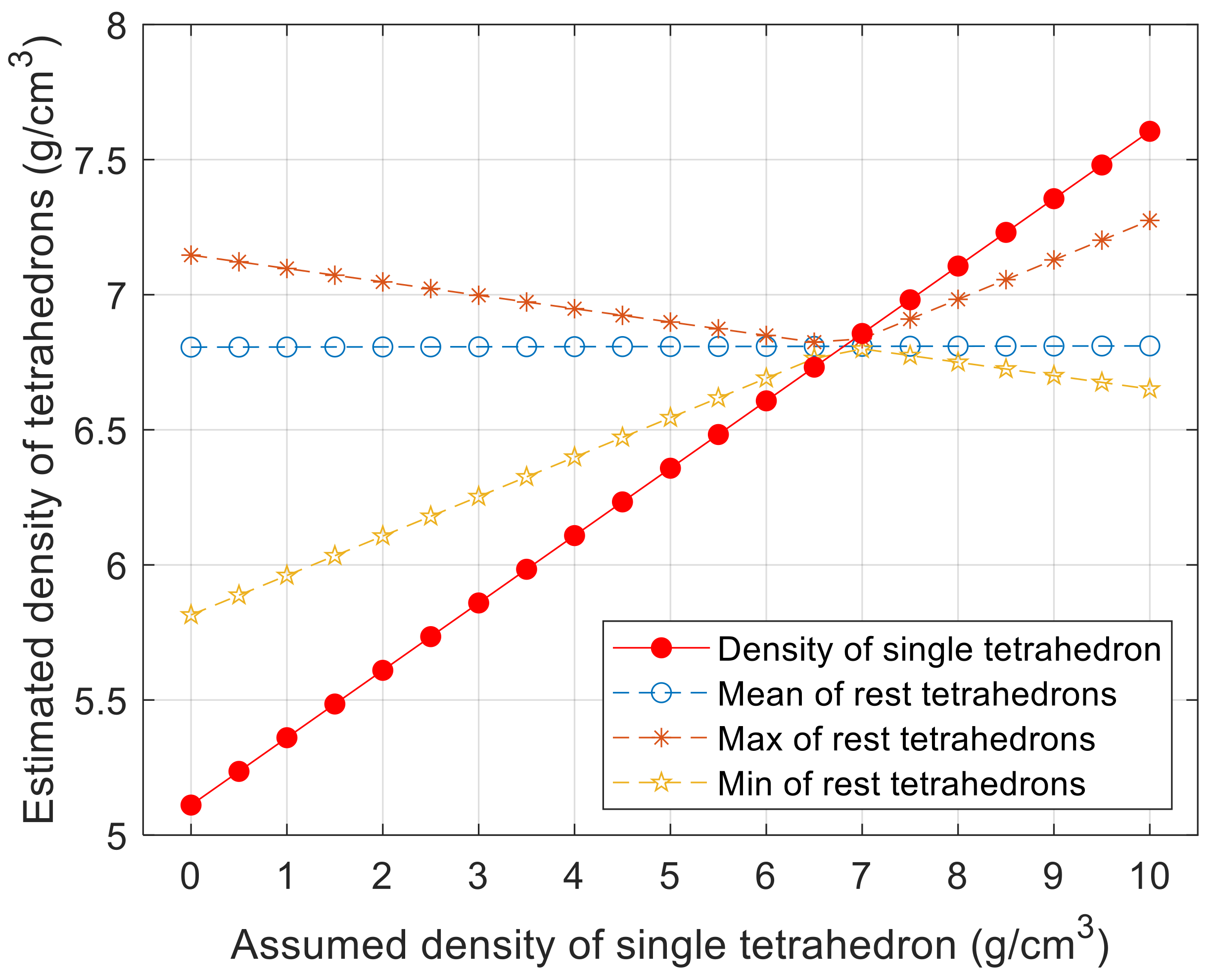
We tested the sensitivity of our approach with the under-determined case (using a single mutation as an example). Tetrahedron No. 1426 was assumed to have an inconstant density from 0 to 10 g / cm 3 , and the densities of the remaining 1466 tetrahedrons were 6.809 g / cm 3 . The true spherical harmonic gravitational field was assigned to degree and order 8. The density of all 1467 tetrahedrons was initialized and assumed to be equal to 6.809 g / cm 3 . We computed the correction to this initial assumption.
Figure 5 shows the estimated density of tetrahedron No. 1426 and the minimum, maximum, and mean of the other 1466 tetrahedrons as a function of the assumed density of that tetrahedron. The red solid line with the red points is the estimated density of tetrahedron No. 1426, and the blue dotted line with the blue circle is the mean value of the remaining tetrahedrons. The yellow and magenta dotted lines with symbols of the yellow star and the magenta asterisk show the minimum and maximum values of the remaining tetrahedrons, respectively. Table 1 lists the absolute error of the estimated density of tetrahedron No. 1426. The results show that, when the density of a tetrahedron is different from the others in an under-determined system, we can separate it from other tetrahedrons, although the density of the special tetrahedron cannot be restored accurately. In particular, when the assumed value is very close to the initial value, the accuracy of density estimation is the best.

4.1.3. Influence of High-Order Spherical Harmonics

In these tests, the influence of the different degrees and orders of the spherical harmonic coefficients on the results of estimating different number density mutations were inspected. Under the premise of three density mutation assumptions (single mutation, double mutations, and ten mutations), we assumed that the densities of the tetrahedrons with density mutations were 10 g / cm 3 , and the density of the other 1466/1465 and 1657 tetrahedrons was assumed to be 6.809 g / cm 3 , respectively. The true spherical harmonic gravitational field was specified up to degree and order 40. Then, we initially assumed that the densities of all 1467 tetrahedrons were equal to the bulk density 6.809 g / cm 3 and calculated the correction for these initial values under the three density mutation assumptions cases. The density estimation results of the mutations and the other tetrahedrons as a function of the harmonic degree used for the “true” gravity field are shown in Figure 6, Figure 7 and 
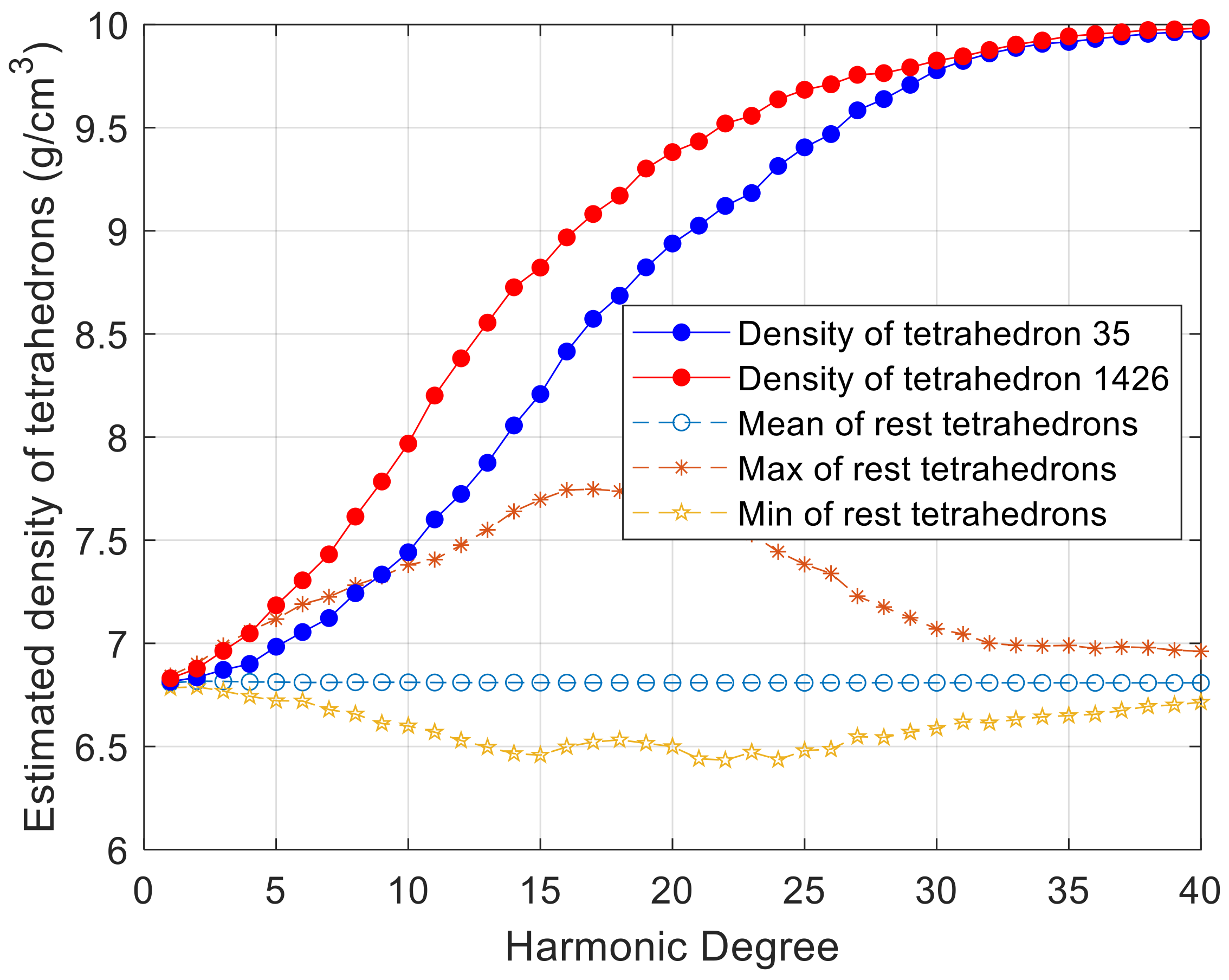
Figure 8, respectively. The solid lines of the three figures show the estimated densities of the mutational tetrahedrons, and the dotted lines with the blue circle, the yellow star, and the magenta asterisk represent the mean, minimum and maximum values of the remaining tetrahedrons, respectively. Table 2 shows the error statistics of the mutations for three density mutation assumptions (we chose degrees 8, 15, 20, and 40 as examples). Figure 9 shows the density estimation results for the three mutation cases by the spherical harmonic gravitational field with degree and order 20. The left plot is the density of each tetrahedron, and the right plot shows the locations of the tetrahedrons, in which the density value is higher as the color becomes closer to yellow.
It should be noted that the densities of the mutant tetrahedrons were estimated more accurately as the degree became higher. In contrast, as the number of mutant tetrahedrons increased and their position distribution in the asteroid became increasingly random, the error of density estimation grew. When the spherical harmonic coefficients increased from degree 1 to 40, the density of the single mutation (tetrahedron No. 1426) was estimated from 6.833 g / cm 3 to 9.984 g / cm 3 , moving closer to the assumed density. Meanwhile, the density of tetrahedron No. 35 with the double mutations increased from 6.815 g / cm 3 to 9.967 g / cm 3 , and the estimated error of ten mutations also increased as the degree became larger.
Comparing the results in Figure 9 with the prior density distributions in Figure 4, it can be found that, when the least-squares method is applied, the density of the mutational tetrahedron can be well estimated. However, we can also see that the densities of the surrounding tetrahedrons will be significantly affected by the mutant tetrahedron, while the tetrahedrons far away from this mutant tetrahedron are almost unaffected. The maximum density of the remaining tetrahedrons is bigger than tetrahedron No. 35 when the harmonic degree is less than 10, as shown in Figure 7. The reason for this is that, due to the close distance between the mutation and its adjacent tetrahedron, it is difficult to distinguish the mutation during the density estimation process. Furthermore, as the degree of the harmonic coefficients is lower, the “measured” gravity field contains less information. Thus, the estimated densities of some tetrahedrons adjacent to the mutation are similar to those of the corresponding mutant, which could be larger than the other tetrahedrons. In addition, to balance the values of the spherical harmonic coefficients of the whole asteroid, some tetrahedrons near the mutation have density values that should be smaller than the other tetrahedrons.
In particular, from the results of the ten mutations case shown in Figure 8 and Figure 9, we can find that the estimated densities of the tetrahedrons, which are closer to the ends of the asteroid, are more accurate than the others, such as tetrahedrons No. 2/35/1401 and 1426. The densities of the tetrahedrons, which are close to the center of the asteroid, such as No. 624/675/790, were estimated to be no more than 8 g / cm 3 —that is, only about 1 g / cm 3 larger than the mean of the remaining tetrahedrons without density mutations.
The above results can be explained by the appearance of the dumbbell-shaped asteroid Kleopatra. A tetrahedron close to the center of an asteroid could be called a near-center tetrahedron; on the contrary, the tetrahedrons distributed at both ends could be called distal tetrahedrons. Since the size of the tetrahedral element is relatively uniform in the model used in this study, the gravitational perturbation caused by the tetrahedron around the near-center tetrahedron is very close to it. Furthermore, it is difficult to distinguish whether the difference in the gravitational potential caused by the density mutation is caused by the mutational tetrahedron or its adjacent tetrahedrons. At the same time, this also explains that, even when the degree of the spherical harmonic coefficients is 40, the density of each tetrahedron cannot be solved accurately. The dimension of the equations is ( 40 + 1 ) 2 1 , which is more than the number of tetrahedral elements, at 1467. Due to the existence of near-centered tetrahedrons, Equation (23) is easily linearly related. Therefore, a positive definite system and a unique equation solution cannot be obtained.
The results show that the spherical harmonic coefficients can be used to estimate the density distribution of asteroids. When mutations of density exist inside an asteroid, they can be detected. If the mutation is in a distal tetrahedron, the density can be estimated accurately, while for a near-center tetrahedron, the density anomaly near it can be estimated.

4.2. Density Distribution Estimation for Known Structures

If a structural hypothesis of asteroids can be obtained through other detection methods, estimating the densities of the known structures will be easier than assuming each tetrahedron is an unknown variable. In this section, it is assumed that we are exploring the asteroid 216 Kleopatra and its internal structure has been ascertained. It is, therefore, necessary to estimate the density of each constituent structure.
We refer to the one- and two-core models proposed in [23] and combine them to form a new structure, as shown in Figure 10. Assuming sphere structures with a radius of 10 km at the center and both ends of the target asteroid, the density near the center of mass is 10 g / cm 3 , the density of the end along the positive x-axis is 8 g / cm 3 , and the density of the end along the negative x-axis is 0. Then, the entire asteroid model is divided into four parts with different densities. It is important to state that, when dividing the four parts, they are not strict spheres. Judging the property of the tetrahedron is based on whether the center of the tetrahedron element is within the spherical range of the given structure. For this process, fine meshing can be used to obtain more precise structural divisions in the future.
Since there are only four unknowns, the system is positive definite, and all the densities can be solved accurately using the appropriate degree and order of spherical harmonic coefficients. The errors of the four parts are shown in Figure 11. When the degree is more than 2, the errors can reach the order of 10 13 g / cm 3 . However, when the degree of the coefficient is 1, we cannot obtain a precise result. As the dimension of Equation (21) is three, it is less than the number of unknowns (four), leading to an under-determined system.
The density data are not listed, but the density distribution of the hypothetical structure in the model is given, as shown in the cross-sectional view of Figure 12 (different colors correspond to different density values). Therefore, as long as the true spherical harmonic coefficients are obtained during the exploration, the density distribution of the asteroid with a known structure can be effectively estimated.

5. Conclusions

This study proposed a free-vertex tetrahedral finite element representation, which is intended to study the internal density distribution of asteroids. The explicit formulation of the free-vertex representation was obtained, based upon which we derived its transformation to the spherical harmonics, enabling us to estimate the internal structure of a massive body from its external gravitational field. The performance of the density distribution was evaluated with the asteroid 216 Kleopatra as an example, showing that: (1) under the condition of only the gravity field and shape data of the asteroid being available, the free-vertex tetrahedral FEM can be used to randomly model the interior of the asteroid, and the density mutation inside the asteroid can be detected; and (2) when otherwise known for the internal structure of the asteroid, the free-vertex tetrahedral FEM can be associated with the corresponding structure, and the density can be estimated accurately. Although the current results exhibited the potential of this free-vertex tetrahedral FEM for estimating the internal structure of an asteroid, we also remarked that the accuracy of the density mutation estimate is related to the location. For the benchmarking test, the density estimation becomes more accurate as the mutations approach the two ends of the asteroid and the density of the near-center meshes is difficult to distinguish using our method.

Author Contributions

Conceptualization, W.Y. and Y.Y.; methodology, W.Y.; software, W.Y.; validation, L.S.; formal analysis, W.Y. and L.S.; investigation, W.Y.; resources, W.Y. and Y.Y.; data curation, W.Y.; writing—original draft preparation, W.Y.; writing—review and editing, Y.S. and Y.Y.; visualization, W.Y.; supervision, L.S. and Y.S. All authors have read and agreed to the published version of the manuscript.

Funding

This research was funded by the National Natural Science Foundation of China under Grants 12003054 and 12022212 and the Advanced Study Program by the Chinese Academy of Sciences (Grant No. CSU-QZKT-2019-05).

Institutional Review Board Statement

Not applicable.

Informed Consent Statement

Not applicable.

Data Availability Statement

Not applicable.

Conflicts of Interest

The authors declare no conflict of interest.

Appendix A. Examples of the Tetranomial Coefficients

The integrands c ¯ n , m and s ¯ n , m should be calculated using the standard simplex coordinates. x , y , z in Equation (7) need to be replaced by u 0 , u 1 , u 2 , u 3 . However, the final expression of the integrands c ¯ n , m and s ¯ n , m contains two sets of tetranomial coefficients, which is not an explicit expression. Below is an example of the u 0 , u 1 , u 2 , u 3 tetranomial coefficients α ¯ h , j , k , l and β ¯ h , j , k , l when the degree and order of the harmonic coefficients are both equal to 1.
When n = 1 and m = 1 , the variable substitution process of the integrands c ¯ 1 , 1 and s ¯ 1 , 1 is given by
c ¯ 1 , 1 s ¯ 1 , 1 = 1 3 M x x r e r e y y r e r e 1 3 M x 1 u 1 + x 2 u 2 + x 3 u 3 + x 0 u 0 r e y 1 u 1 + y 2 u 2 + y 3 u 3 + y 0 u 0 r e
Therefore, the integrands c ¯ 1 , 1 and s ¯ 1 , 1 can be rewritten as
c ¯ 1 , 1 s ¯ 1 , 1 = 1 3 M · r e x 1 u 0 0 u 1 1 u 2 0 u 3 0 + x 2 u 0 0 u 1 0 u 2 1 u 3 0 + x 3 u 0 0 u 1 0 u 2 0 u 3 1 + x 0 u 0 1 u 1 0 u 2 0 u 3 0 y 1 u 0 0 u 1 1 u 2 0 u 3 0 + y 2 u 0 0 u 1 0 u 2 1 u 3 0 + y 3 u 0 0 u 1 0 u 2 0 u 3 1 + y 0 u 0 1 u 1 0 u 2 0 u 3 0
The tetranomial coefficients can be written as
α ¯ 0 , 1 , 0 , 0 = x 1 3 M · r e , α ¯ 0 , 0 , 1 , 0 = x 2 3 M · r e , α ¯ 0 , 0 , 0 , 1 = x 3 3 M · r e , α ¯ 1 , 0 , 0 , 0 = x 0 3 M · r e β ¯ 0 , 1 , 0 , 0 = y 1 3 M · r e , β ¯ 0 , 0 , 1 , 0 = y 2 3 M · r e , β ¯ 0 , 0 , 0 , 1 = y 3 3 M · r e , β ¯ 1 , 0 , 0 , 0 = y 0 3 M · r e
Then, c ¯ 1 , 1 and s ¯ 1 , 1 can be rewritten as
c ¯ 1 , 1 s ¯ 1 , 1 = α ¯ 0 , 1 , 0 , 0 u 0 0 u 1 1 u 2 0 u 3 0 + α ¯ 0 , 0 , 1 , 0 u 0 0 u 1 0 u 2 1 u 3 0 + α ¯ 0 , 0 , 0 , 1 u 0 0 u 1 0 u 2 0 u 3 1 + α ¯ 1 , 0 , 0 , 0 u 0 1 u 1 0 u 2 0 u 3 0 β ¯ 0 , 1 , 0 , 0 u 0 0 u 1 1 u 2 0 u 3 0 + β ¯ 0 , 0 , 1 , 0 u 0 0 u 1 0 u 2 1 u 3 0 + β ¯ 0 , 0 , 0 , 1 u 0 0 u 1 0 u 2 0 u 3 1 + β ¯ 1 , 0 , 0 , 0 u 0 1 u 1 0 u 2 0 u 3 0
Repeating the above variable substitution process, we can obtain all the tetranomial coefficients α ¯ h , j , k , l and β ¯ h , j , k , l at any degree and order. The integrands c ¯ n , m and s ¯ n , m can be abbreviated as
c ¯ n , m u 0 , u 1 , u 2 , u 3 s ¯ n , m u 0 , u 1 , u 2 , u 3 = i 0 + i 1 + i 2 + i 3 = n α ¯ i 0 , i 1 , i 2 , i 3 β ¯ i 0 , i 1 , i 2 , i 3 u 0 i 0 u 1 i 1 u 2 i 2 u 3 i 3

Appendix B. Simplex Integral

The simplex (the tetrahedral finite element) has the simplest shape in each dimension space, such as a point for zero dimension, a directed line segment for one-dimensional space, and a directed triangle for two-dimensional space; for three-dimensional space, it is a tetrahedron. Unlike ordinary definite integrals, simplex integrals use a simplex as the integration domain, which can be divided into positive and negative directions. The simplex used in this study is the three-dimensional simplex if there are no special instructions.
The three-dimensional simplex integral expression is
S = U 0 U 1 U 2 U 3 u 0 i 0 u 1 i 1 u 2 i 2 u 3 i 3 d u 1 d u 2 d u 3
It can be expanded as
S = u 0 , u 1 , u 2 , u 3 0 u 0 + u 1 + u 2 + u 3 = 1 u 0 i 0 u 1 i 1 u 2 i 2 u 3 i 3 d u 1 d u 2 d u 3 = 0 1 0 1 u 3 0 1 u 3 u 2 u 0 i 0 u 1 i 1 u 2 i 2 u 3 i 3 d u 1 d u 2 d u 3 = 0 1 0 1 u 3 u 3 i 3 u 2 i 2 0 1 u 3 u 2 u 1 i 1 1 u 3 u 2 u 1 i 0 d u 1 d u 2 d u 3
The internal integration can be calculated using partial integration:
0 1 u 3 u 2 u 1 i 1 1 u 3 u 2 u 1 i 0 d u 1 = 0 1 u 3 u 2 d 1 i 1 + 1 u 1 i 1 + 1 1 u 3 u 2 u 1 i 0 = 1 i 1 + 1 u 1 i 1 + 1 1 u 3 u 2 u 1 i 0 0 1 u 3 u 2 0 1 u 3 u 2 1 i 1 + 1 u 1 i 1 + 1 d 1 u 3 u 2 u 1 i 0 = 0 1 u 3 u 2 1 i 1 + 1 u 1 i 1 + 1 d 1 u 3 u 2 u 1 i 0 = 0 1 u 3 u 2 i 0 i 1 + 1 u 1 i 1 + 1 1 u 3 u 2 u 1 i 0 1 d u 1 = 0 1 u 3 u 2 i 0 i 0 1 i 1 + 1 i 1 + 2 u 1 i 1 + 2 1 u 3 u 2 u 1 i 0 2 d u 1 = 0 1 u 3 u 2 i 0 i 0 1 i 0 2 i 1 + 1 i 1 + 2 i 1 + 3 u 1 i 1 + 3 1 u 3 u 2 u 1 i 0 3 d u 1 = 0 1 u 3 u 2 i 0 i 0 1 i 0 2 2 i 1 + 1 i 1 + 2 i 1 + 3 i 1 + i 0 1 u 1 i 1 + i 0 1 × 1 u 3 u 2 u 1 1 d u 1 = 0 1 u 3 u 2 i 0 i 0 1 i 0 2 1 i 1 + 1 i 1 + 2 i 1 + 3 i 1 + i 0 u 1 i 1 + i 0 d u 1 = 0 1 u 3 u 2 i 0 ! i 1 ! i 1 + i 0 ! u 1 i 1 + i 0 d u 1 = 0 1 u 3 u 2 i 0 ! i 1 ! i 1 + i 0 + 1 ! d u 1 i + i 0 + 1 = i 0 ! i 1 ! i 1 + i 0 + 1 ! u 1 i 1 + i 0 + 1 0 1 u 3 u 2 = i 0 ! i 1 ! i 1 + i 0 + 1 ! 1 u 3 u 2 i + i 0 + 1
The simplex integral can eventually be obtained by repeating the partial integration to Equation (A7):
S = 0 1 0 1 u 3 u 3 i 3 u 2 i 2 d u 2 d u 3 0 1 u 3 u 2 u 1 i 1 1 u 3 u 2 u 1 i 0 d u 1 = 0 1 u 3 i 3 0 1 u 3 u 2 i 2 1 u 3 u 2 i 1 + i 0 + 1 d u 2 d u 3 i 0 ! i 1 ! i 1 + i 0 + 1 ! = 0 1 u 3 i 3 1 u 3 i 2 + i 1 + i 0 + 1 d u 3 i 0 ! i 1 ! i ! i 2 + i 1 + i 0 + 2 ! = i 0 ! i 1 ! i 2 ! i ! i 3 + i 2 + i 1 + i 0 + 3 !

Appendix C. Hammer Integral

Finite element numerical integration obtains approximate numerical integration results by selecting several special integration points and weight coefficients on the standard simplex. The Hammer integral uses an interpolation function and assumes its value change law to be between grids to calculate an approximate solution. Therefore, the accuracy of the numerical algorithm is slightly worse than that of the simplex integral, but the calculation efficiency is greater. In the finite element method, the three-dimensional simplex integral of Equation (A6) can be expressed as
I = 0 1 0 1 L 1 0 1 L 2 L 1 F I 1 , L 2 , L 3 , L 4 d L 3 d L 2 d L 1
Table A1. The coordinates of the integration points, weighting coefficients and error magnitudes of the three-dimensional tetrahedral element.
Number of
Integration Points
Weighting CoefficientsCoordinates of
the Integration Points
Error
Magnitude
1A1 = 11/4,1/4,1/4,1/4O (h2)
4B4 = 1/4a = 0.58541020
b = 0.13819660
O (h3)
5A1 = −4/5
B4 = 9/20
a = 1/2
b = 1/6
O (h4)
Given the coordinates of the integration points, weighting coefficients, and error magnitudes of the three-dimensional tetrahedral element through Table A1, and the numerical integration can be derived as
0 1 0 1 L 1 0 1 L 1 L 2 F L 1 , L 2 , L 2 , L 4 d L 3 d L 2 d L 1 = A 1 F 1 4 , 1 4 , 1 4 , 1 4 + B 4 { F ( a , b , b , b ) + F ( b , a , b , b ) + F ( b , b , a , b ) + F ( b , b , b , a )

References

  1. Carry, B. Density of asteroids. Planet. Space Sci. 2012, 73, 98–118. [Google Scholar] [CrossRef] [Green Version]
  2. Durante, D.; Hemingway, D.; Racioppa, P.; Iess, L.; Stevenson, D. Titan’s gravity field and interior structure after Cassini. Icarus 2019, 326, 123–132. [Google Scholar] [CrossRef] [Green Version]
  3. Cappuccio, P.; Hickey, A.; Durante, D.; Di Benedetto, M.; Iess, L.; De Marchi, F.; Plainaki, C.; Milillo, A.; Mura, A. Ganymede’s gravity, tides and rotational state from JUICE’s 3GM experiment simulation. Planet. Space Sci. 2020, 187, 104902. [Google Scholar] [CrossRef]
  4. Yeomans, D.; Antreasian, P.; Barriot, J.P.; Chesley, S.; Dunham, D.; Farquhar, R.; Giorgini, J.; Helfrich, C.; Konopliv, A.; McAdams, J.; et al. Radio science results during the NEAR-Shoemaker spacecraft rendezvous with Eros. Science 2000, 289, 2085–2088. [Google Scholar] [CrossRef] [PubMed]
  5. Takeuchi, H.; Yoshikawa, K.; Takei, Y.; Oki, Y.; Kikuchi, S.; Ikeda, H.; Soldini, S.; Ogawa, N.; Mimasu, Y.; Ono, G.; et al. The deep-space multi-object orbit determination system and its application to Hayabusa2’s asteroid proximity operations. Astrodynamics 2020, 4, 377–392. [Google Scholar] [CrossRef]
  6. McMahon, J.; Scheeres, D.; Hesar, S.; Farnocchia, D.; Chesley, S.; Lauretta, D. The OSIRIS-REx radio science experiment at Bennu. Space Sci. Rev. 2018, 214, 43. [Google Scholar] [CrossRef]
  7. Walsh, K.J. Rubble pile asteroids. Annu. Rev. Astron. Astrophys. 2018, 56, 593–624. [Google Scholar] [CrossRef] [Green Version]
  8. Circi, C.; D’Ambrosio, A.; Lei, H.; Ortore, E. Global mapping of asteroids by frozen orbits: The case of 216 kleopatra. Acta Astronaut. 2019, 161, 101–107. [Google Scholar] [CrossRef]
  9. Kaula, W.M. Theory of Satellite Geodesy: Applications of Satellites to Geodesy; Courier Corporation: Waltham, MA, USA, 2000. [Google Scholar]
  10. Werner, R.A.; Scheeres, D.J. Exterior gravitation of a polyhedron derived and compared with harmonic and mascon gravitation representations of asteroid 4769 Castalia. Celest. Mech. Dyn. Astron. 1996, 65, 313–344. [Google Scholar] [CrossRef]
  11. Chanut, T.; Aljbaae, S.; Carruba, V. Mascon gravitation model using a shaped polyhedral source. Mon. Not. R. Astron. Soc. 2015, 450, 3742–3749. [Google Scholar] [CrossRef]
  12. Romain, G.; Jean-Pierre, B. Ellipsoidal harmonic expansions of the gravitational potential: Theory and application. Celest. Mech. Dyn. Astron. 2001, 79, 235–275. [Google Scholar] [CrossRef]
  13. Herrera-Sucarrat, E.; Palmer, P.; Roberts, R. Modeling the gravitational potential of a nonspherical asteroid. J. Guid. Control Dyn. 2013, 36, 790–798. [Google Scholar] [CrossRef] [Green Version]
  14. Colombi, A.; Hirani, A.N.; Villac, B.F. Adaptive gravitational force representation for fast trajectory propagation near small bodies. J. Guid. Control Dyn. 2008, 31, 1041–1051. [Google Scholar] [CrossRef] [Green Version]
  15. Wei, B.; Shang, H.; Qiao, D. Hybrid model of gravitational fields around small bodies for efficient trajectory propagations. J. Guid. Control Dyn. 2020, 43, 232–249. [Google Scholar] [CrossRef]
  16. Scheeres, D.; Khushalani, B.; Werner, R.A. Estimating asteroid density distributions from shape and gravity information. Planet. Space Sci. 2000, 48, 965–971. [Google Scholar] [CrossRef]
  17. Yin, W.; Shu, L.; Yu, Y.; Gao, Y. Use of Tetrahedral Finite Element Method for Computing the Gravitation of Irregular-Shaped Asteroid. In IOP Conference Series: Materials Science and Engineering; IOP Publishing: Philadelphia, PA, USA, 2019; Volume 608, p. 012043. [Google Scholar]
  18. Yu, Y.; Cheng, B.; Hayabayashi, M.; Michel, P.; Baoyin, H. A finite element method for computational full two-body problem: I. The mutual potential and derivatives over bilinear tetrahedron elements. Celest. Mech. Dyn. Astron. 2019, 131, 51. [Google Scholar] [CrossRef]
  19. Michel, P.; Benz, W.; Tanga, P.; Richardson, D.C. Collisions and gravitational reaccumulation: Forming asteroid families and satellites. Science 2001, 294, 1696–1700. [Google Scholar] [CrossRef] [PubMed] [Green Version]
  20. Yu, Y.; Richardson, D.C.; Michel, P. Structural analysis of rubble-pile asteroids applied to collisional evolution. Astrodynamics 2017, 1, 57–69. [Google Scholar] [CrossRef] [Green Version]
  21. Hu, S.; Ji, J.; Richardson, D.C.; Zhao, Y.; Zhang, Y. The formation mechanism of 4179 Toutatis’ elongated bilobed structure in a close Earth encounter scenario. Mon. Not. R. Astron. Soc. 2018, 478, 501–515. [Google Scholar] [CrossRef] [Green Version]
  22. Massironi, M.; Simioni, E.; Marzari, F.; Cremonese, G.; Giacomini, L.; Pajola, M.; Jorda, L.; Naletto, G.; Lowry, S.; El-Maarry, M.R.; et al. Two independent and primitive envelopes of the bilobate nucleus of comet 67P. Nature 2015, 526, 402–405. [Google Scholar] [CrossRef] [Green Version]
  23. Takahashi, Y.; Scheeres, D.J. Small body surface gravity field estimation from orbit determination. Adv. Astronaut. Sci. 2011, 141, 323–340. [Google Scholar]
  24. Pearl, J.M.; Hitt, D.L. Asteroid gravitational models using mascons derived from polyhedral sources. In Proceedings of the AIAA/AAS Astrodynamics Specialist Conference, Long Beach, CA, USA, 12–15 September 2016; p. 5260. [Google Scholar]
  25. Pearl, J.; Hitt, D. Comparing the computational efficiency of polyhedral and mascon gravity models. In Proceedings of the 27th AIAA/AAS Spaceflight Mechanics Meeting, San Antonio, TX, USA, 5–9 February 2017. [Google Scholar]
  26. Rathinam, A.; Dempster, A.G. Octree-Based Mascon Model for Small Body Gravity Fields. J. Guid. Control Dyn. 2019, 42, 2557–2567. [Google Scholar] [CrossRef]
  27. Park, R.S.; Werner, R.A.; Bhaskaran, S. Estimating small-body gravity field from shape model and navigation data. J. Guid. Control Dyn. 2010, 33, 212–221. [Google Scholar] [CrossRef]
  28. Takahashi, Y.; Scheeres, D. Morphology driven density distribution estimation for small bodies. Icarus 2014, 233, 179–193. [Google Scholar] [CrossRef]
  29. Ledbetter, W.; Sood, R.; Stuart, J. Expected Accuracy of Density Recovery Using Satellite Swarm Gravity Measurements. In Proceedings of the AAS/AIAA Space Flight Mechanics Meeting, Maui, HI, USA, 13–17 January 2019. [Google Scholar]
  30. Ostro, S.J.; Scott, R.; Hudson, M.C.N.; Margot, J.L.; Scheeres, D.J.; Campbell, D.B.; Magri, C.; Giorgini, J.D.; Yeomans, D.K. Radar observations of asteroid 216 Kleopatra. Science 2000, 288, 836–839. [Google Scholar] [CrossRef] [Green Version]
  31. Cheng, S.W.; Dey, T.; Shewchuk, J. Delaunay Mesh Generation; CRC Press: Boca Raton, FL, USA, 2016; pp. 1–386. [Google Scholar]
  32. Ming-yong, L.C.K.P. An Algorithm for Generating Tetrahedral Mesh Based on Octree. Microcomput. Inf. 2010, 24, 174–175. [Google Scholar]
  33. Peraire, J.; Peiro, J.; Formaggia, L.; Morgan, K.; Zienkiewicz, O.C. Finite element Euler computations in three dimensions. Int. J. Numer. Methods Eng. 1988, 26, 2135–2159. [Google Scholar] [CrossRef]
  34. Saiki, T.; Mimasu, Y.; Takei, Y.; Yamada, M.; Sawada, H.; Ogawa, K.; Ogawa, N.; Takeuchi, H.; Miura, A.; Shimaki, Y.; et al. Motion reconstruction of the small carry-on impactor aboard Hayabusa. Astrodynamics 2020, 4, 289–308. [Google Scholar] [CrossRef]
  35. Werner, R.A. Spherical harmonic coefficients for the potential of a constant-density polyhedron. Comput. Geosci. 1997, 23, 1071–1077. [Google Scholar] [CrossRef]
  36. Li, Q.; Zheng, J.; Liao, G.; Jin, Y. Approach on area coordinate, volume coordinate and their application in true 3DGIS. J. Earth Sci. Eng. 2011, 1, 52–59. [Google Scholar]
  37. Jacob, F.; Ted, B. A First Course in Finite Elements; Wiley: Hoboken, NJ, USA, 2007. [Google Scholar]
  38. Hammer, P.C.; Stroud, A.H. Numerical integration over simplexes. Math. Tables Other Aids Comput. 1956, 10, 137–139. [Google Scholar] [CrossRef]
  39. Hammer, P.C.; Stroud, A.H. Numerical evaluation of multiple integrals II. Math. Tables Other Aids Comput. 1958, 12, 272–280. [Google Scholar] [CrossRef]
  40. Saylor, P.E. Use of the singular value decomposition with the Manteuffel algorithm for nonsymmetric linear systems. SIAM J. Sci. Stat. Comput. 1980, 1, 210–222. [Google Scholar] [CrossRef]
Figure 1. Tetrahedral finite elements: (a) centroid-vertex; (b) free-vertex.
Aerospace 08 00371 g001
Figure 2. Triangular out-of-plane normal direction vector and edge normal direction vector.
Aerospace 08 00371 g002
Figure 3. The asteroid 216 Kleopatra shape model: (a) the shape model; (b) polyhedron model; (c) free-vertex tetrahedral FEM with 1467 tetrahedrons (sectional plane); (d) free-vertex tetrahedral FEM with 160,217 tetrahedrons (sectional plane) (the color corresponds to the size of the tetrahedron: green means a large size, and red means a small size).
Aerospace 08 00371 g003
Figure 4. Density distribution assumption: (a) density value; (b) location of density mutation.
Aerospace 08 00371 g004
Figure 5. Density distribution estimation solution as a function of the assumed density with the single tetrahedron numbered 1426.
Aerospace 08 00371 g005
Figure 6. Density estimation solution as a function of the degree and order of the measured gravitational field, computed for the single mutation.
Aerospace 08 00371 g006
Figure 7. Density estimation solution as a function of the degree and order of the measured gravitational field, computed for the double mutations.
Aerospace 08 00371 g007
Figure 8. Density estimation solution as a function of the degree and order of the measured gravitational field, computed for the 10 mutations.
Aerospace 08 00371 g008
Figure 9. Density results for the three cases of density mutations by the spherical harmonic gravitational field with degree and order 20: (a) density value; (b) location of density mutation.
Aerospace 08 00371 g009
Figure 10. Assumed structure of asteroid 216 Kleopatra.
Aerospace 08 00371 g010
Figure 11. Density errors of the four parts with a gravitational field of degree and order 1 to 8.
Aerospace 08 00371 g011
Figure 12. The density distribution of the known structure in the cross-sectional view.
Aerospace 08 00371 g012
Table 1. Validation test result of the single-mutation case.
Assumed Density
of Tetrahedron
No. 1426 (g/ cm 3 )
Estimated Density
of Tetrahedron
No. 1426 (g/ cm 3 )
Absolute Error of the
Estimated Density of
Tetrahedron No. 1426 (g/ cm 3 )
05.11115.1111
15.36044.3604
25.60983.6098
35.85922.8592
46.10852.1085
56.35791.3579
66.60730.6073
76.85660.1434
87.10590.8940
97.35541.6446
107.60472.3953
Table 2. The error statistics of the mutations for three density mutation assumptions.
Degree of
Harmonics
Coefficients
Single
Mutation
Double Mutations10 Mutations
No. 1426
g/ cm 3
No. 35
g/ cm 3
No. 1426
g/ cm 3
Mean
g/ cm 3
Mean
g/ cm 3
Max
g/ cm 3
Min
g/ cm 3
82.39522.75692.38522.57112.88803.10152.5712
151.16141.79141.17821.48482.11383.04531.1184
200.61931.06160.61840.83991.75052.94910.6786
400.01550.03250.01610.02431.21062.8940.0033
Publisher’s Note: MDPI stays neutral with regard to jurisdictional claims in published maps and institutional affiliations.

