1. Introduction
The development of lightweight structures is of great importance in the aeronautical and space sectors, and is progressively becoming more important in all fields of engineering due to the increasing life cycle costs related to raw materials and energy. Composite materials play an important role in lightweight design, and when compared to metallic parts, offer more design freedom. However, they require better optimization methods to find optima, and have additional challenges related to finding optimum material distributions. In the case of thin-walled laminated composite structures, finding this material distribution translates into finding the optimum number of composite layers and their respective orientations. Moreover, the design of composite panels requires finding the optimum number of stiffeners, the optimum geometry for stiffeners and the optimum laminated composite layouts that constitute the skin and stiffeners.
The use of design schemes coupling machine learning techniques with optimization algorithms is not new. Fu et al. [
1] combined neural networks (NN) with genetic algorithms (GA) using mixed continuous-discrete variables, constraining the axial stiffness during the pre- and post-local buckling of the skin panels, and ultimate load. The NN was trained using the finite element method simulating at 266 sampling points. The global optimum was found using the NN coupled with the GA, and the final results were verified against the finite element model. Ehsani and Dalir [
2] also proposed an NN-GA coupled approach to handle mixed continuous-discrete design variables with four continuous variables related to the width and thickness of angle-grid rib-stiffeners, and four discrete variables related to the number and geometric orientation of those stiffening elements. The NN training took 1060 simulations using a Ritz approach. The same authors proposed pure GA optimization [
3] for another gird-stiffened plate with eight continuous and three discrete design variables. In addition, 250 GA generations were used as the stopping criterion, thereby requiring thousands of evaluations to reach a converged solution.
According to the modeling and simulation perspective, an effective way to reduce the time spent on model evaluation is through the use of surrogate techniques, such as response surface and metamodeling tools. A surrogate is included in the optimization cycle in order to approximate the response of a more expensive finite element analysis. Thole and Ramu [
4] proposed a modified self-organizing map algorithm to identify regions of interest (RoI) in the design space. This proposition is useful in the context of building metamodels with limited computational costs. Self-organizing maps are used as a visualization technique for design space exploration that allows the identification of regions of interest. A modified version enabled the identification of the RoI and the addition of new sampling techniques to be used within a Kriging metamodel scheme that supported the optimization cycle. Despite the clear reduction in computational load, the quality of the approximation showed to be highly dependent on the quantity and quality of the data used in the training phase, which is also valid for accelerated Kriging metamodels, recently used by Wang et al. [
5,
6] for finding optimal variable-stiffness layouts of composite filament-would cylinders. Therefore, for a given computational cost, a better overall optimization result is obtained when extra attention is given to the data generation process.
Branched multipoint approximate (BMA) functions proposed by Chen et al. [
7] and An et al. [
8] can also be used to construct approximate responses of real structures. An et al. [
9] proposed the application of BMA functions on the optimization of composite laminated stiffened panels, successfully achieving optimum designs with discrete variables.
Liu et al. [
10] presented a review on adaptive sampling techniques for global metamodeling, where the concept of space filling sampling was explained. The authors highlighted that classic sampling approaches have a long history in the field of design of experiments (DOE), and that their development was motivated by the design of physical experiments, and largely applied to numerical experiments. Then, the discussion of single-response adaptive sampling and multi-response adaptive sampling techniques was outlined, discussing aspects related to initial design space points, stopping criteria and trade-offs between local exploitation and global exploration. The summarized general finding is that adaptive sampling strategies provide useful feedback about the target function, and that there is not a specific strategy that always outperforms.
Support vector machine (SVM) is a classification technique belonging to the realm of machine learning. Among the desirable features are over-fitting avoidance and reduction in the amount of training data needed when compared with the neural network class of algorithms, especially for a multidimensional feature space [
11]. SVM has as its main feature the ability to explicitly define complex decision functions that optimally separate two classes of data samples [
12]. Thus, once the coefficient samples are categorized into two classes, SVM can provide an explicit decision function (the limit state function) separating the distinct classes. Missoum et al. [
13,
14,
15] introduced the notion of an explicitly decomposed design space, whereby the limit state functions are constructed explicitly in terms of the design variables, using SVM.
In reference [
15], the authors introduced an adaptive sampling scheme that reduces the number of function evaluations. The approach is based on SVM and constructs an explicit approximation of the domain boundaries with respect to the design variables. The design space is explicitly decomposed into feasible and infeasible regions. The authors handled the discontinuity of the response using a clustering technique which provides the basic classification for the construction of the SVM decision function. In a follow up study [
16], the authors proposed substantial modifications by improving the choice of samples, and applying a more rigorous convergence criterion and a new technique to select the SVM kernel parameters.
Basudhar and Missoum [
17] also presented a methodology for constrained global optimization, where the boundary of the feasible domain is approximated by a single SVM, and the probability of feasibility is calculated using a new probabilistic SVM model based on a sigmoid function. Two sample selection levels were used: a first stage dedicated to the global search of the constrained optimum; and a second stage focused on the local refinement of the SVM approximating the boundary of the feasible space. Their study introduced and compared an unconstrained and a constrained formulation of SVM-based optimization.
Song et al. [
18] used linear and nonlinear virtual SVM in optimization problems with up to 12 variables with dynamic Kriging, finding that SVM can accurately build the decision function for the purpose of reliability-based analysis, and that SVM becomes more efficient than Kriging for high-dimensional problems.
In classification tasks, based on an independent and distributed training dataset, SVM aims at finding a discriminant function that can predict labels for new instances. From a geometric perspective, computing a classifier is equivalent to finding the equation for a multidimensional surface that best separates the different classes in the feature space. The regression problem is a generalization of the classification problem, in which the model provides a continuous-valued output.
The present paper proposes a new methodology to obtain optimal designs of composite stiffened panels. The panel consists of a representative segment of a wing’s upper skin, whereby the local loads are calculated considering the global wing behavior. The design parameterization considers the number of stiffeners, the geometry of the stiffeners and the composite layup for the stiffeners and the skin. During the optimization, the number of high fidelity samples to be evaluated is guided by a design of experiment (DOE) based on the Latin hypercube algorithm [
19]. The DOE data supports a SVM model that is able to classify between feasible and infeasible designs.
The main scientific contributions of the paper are:
Use a limited and pre-determined number of high-fidelity finite element evaluations based on the DOE requirements;
Use multiple objectives of continuous optimization (in opposition to integer optimization), whereby interpolation and classification objectives are built utilizing SVM models;
Generate a Pareto frontier that discusses the contributions of mass and feasibility (buckling constraint) to the optimal design.
The paper is organized as follows.
Section 2 presents the wing model, load idealization and buckling analysis. The methodology is presented in
Section 3, addressing design parameterization, optimization workflow and data analysis.
Section 4 shows the numerical results. Conclusions are presented in
Section 5.
2. Structural Modeling
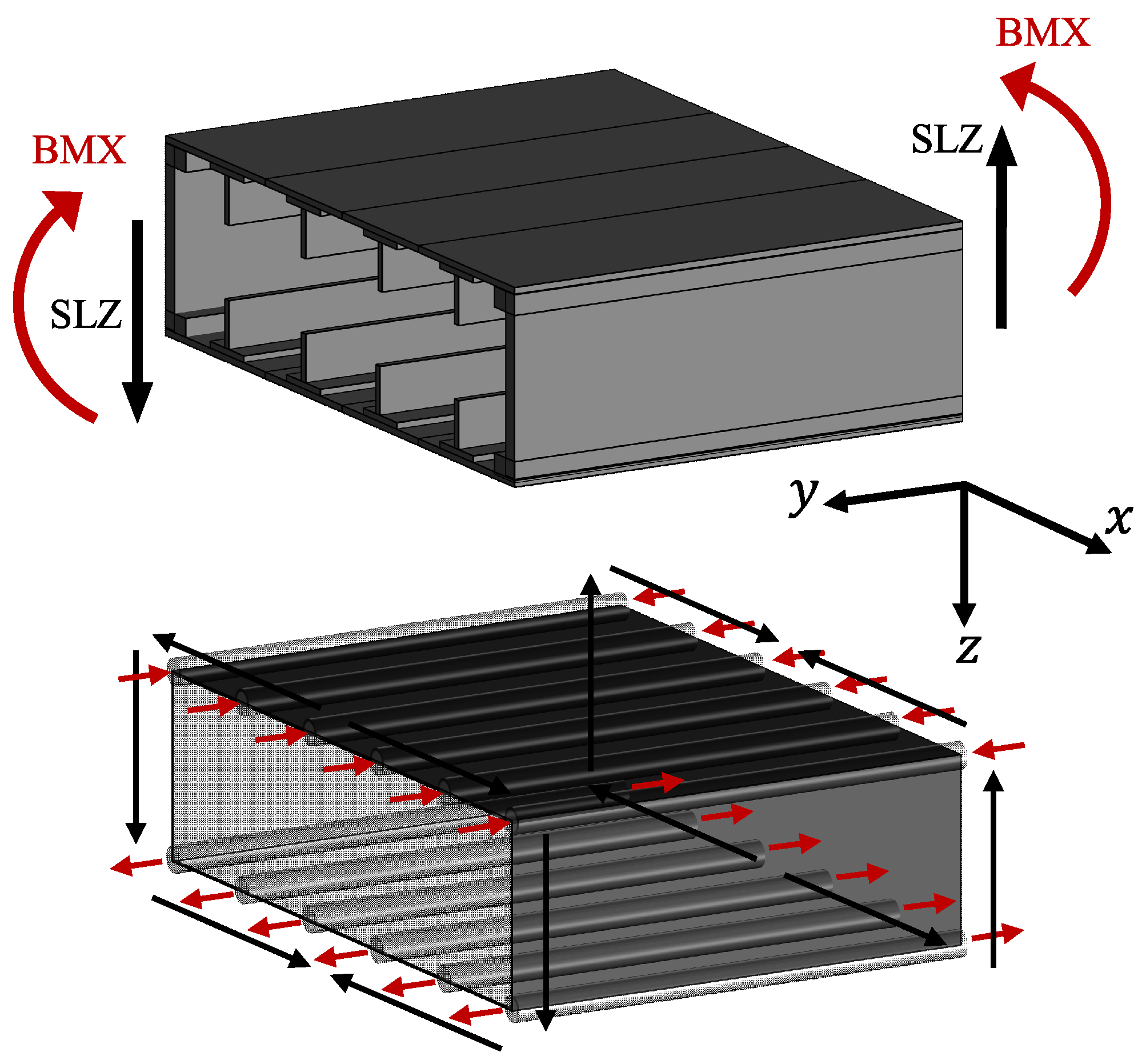
In the present study, only a single up-bending load case was considered, and it was assumed that the distributed load over the wing could be in equilibrium with a bending moment (BMX) and a transverse shear load (SLZ) at the wing root, as illustrated in
Figure 1. These design loads were determined by assuming the wing to be a cantilever beam and subjected to an idealized elliptical lifting load distribution along the half span. The resultant load was derived considering the aircraft maximum take-off weight and maximum flight load factors, resulting in
kNm and
kN for the current study case. Note that the contributions from the wing weight on the bending, the torsion moments and the in-plane bending moment caused mainly by drag forces were ignored.
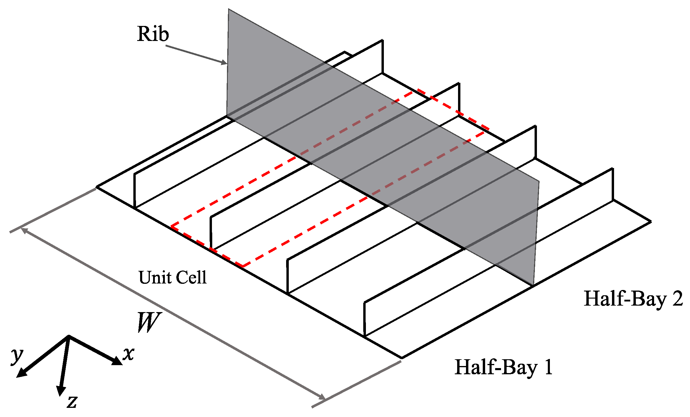
In order to evaluate the structural response at the wing root, a finite element (FE) model was constructed based on a representative cell of a double half-bay model, as proposed by Fenner [
20], which is a stringer-skin assembly consisting of two halves of adjacent wing bays separated by a middle rib, where the nodes have zero normal displacements. Note that any cross-section other than the wing root could have been selected, and the present study focused on the wing root. The representative cell is a fraction of the entire panel and includes one longitudinal stiffener segment attached to the skin. The skin width was equal to the spacing between adjacent stiffener segments. The length of the representative cell extended longitudinally from one adjacent mid-bay to the other, as delimited by the red box region shown in
Figure 2. The representative cell approach is convenient during a preliminary design phase where only few design characteristics are completely defined and frequent design modifications require a rapid tool for concept validation. Machado et al. [
21] coupled this modeling scheme for the optimization of stiffened panels using genetic algorithms.
The FE model of the representative cell is based on general-purpose quadrilateral plate elements with bi-linear displacement interpolation within the element domain. In Nastran, these elements are known as CQUAD4 [
22], having four nodes and six degrees-of-freedom per node, being the translations parallel to
, and the three respective rotations about these three axes. The symmetric boundary condition is used in the four edges, as depicted in
Figure 3. The edges perpendicular to the chord-wise direction are constrained in translation along the
y direction and rotations with respect to the
x and
z-axes. The edges perpendicular to the span-wise direction are constrained in rotation with respect to the
y and
z-axes. Moreover, nodal translations are constrained at the bottom edge in
x direction, and the rib placed in the middle of the representative cell creates a support in the
z direction, such that the corresponding nodes are constrained for normal translations.
The longitudinal stringer is composed of a pair of L-shaped stringers joined in their shared mid-plane to form a T-shape or blade-type stringer, making the laminate at the stringer web symmetric over the mid-plane. Hence, the laminate at the stringer foot is allowed to be asymmetric. With the default setting, MSC Nastran
® [
22] calculates the thickness of the plate element with respect to the reference plane determined by the nodes within the element, creating a symmetrical thickness distribution profile shown in the laminate cross-section. However, the symmetric thickness distribution about the mid-plane is not consistent with the manufacturing of these panels. Thus, in order for the FE model of
Figure 3 to correctly represent the as-manufactured cross-section of
Figure 4, the shell elements representing the skin and stiffener’s base regions must be offset from the reference plane by a value
, with
and
being the local skin and stiffener’s thicknesses. Note that the thickness of the stiffener’s base laminate, i.e., the region connected to the skin, is
.
The properties for carbon-epoxy unidirectional plies used in the present study are extracted from Kassapoglou [
23]
= 137.88 GPa,
= 11.72 GPa,
= 0.3,
= 4.825 GPa,
= 1600 kg/m
3 and
= 0.1524 mm.
2.1. Load Idealization
In a preliminary design, it is desirable to have a rapid and accurate method to calculate loads for a representative cell of the panel. A structural idealization of the wing root cross-section was employed according to Megson [
24], where the longitudinal stiffeners were treated as concentrated areas carrying only axial stresses, whereas the idealized skin carried the shear stresses. The bending stresses were determined by:
where
of
Figure 5;
in the present work;
are second moments of area calculated using the idealized cross-section. The design loads
kNm and
kN previously mentioned were used in the wing bay optimization process. The shear flow distribution over the idealized wing section
was determined by Equation (
2)
where
is the shear flow induced in an equivalent virtually opened section and
a correction shear flow. For any given section,
was calculated by virtually crating a cut that opened the closed section, and using the concentrated areas
with their respective positions in the idealized section, as per Equation (
3):
The term
in Equation (
2) is determined from the equilibrium of moments given in Equation (
4)
where the equilibrium is taken from an arbitrary axis. The left-hand side represents the moment of the external shear forces
and
, which are offset from the moment axis by
and
, measured, respectively, in the
z and
x axes. The closed integral on the right-hand side represents the moments generated by the shear flow distribution
, calculated per Equation (
3); and the area
A corresponds to the area enclosed by the idealized section.
The idealized cross-section discretization and calculation of local axial and shear stresses are particularly interesting in the present study, as the actual wing bay section had to be discretized into booms to determine stress acting on the skin, based on the geometrical parameters from the skin and stiffener. In the optimization problem, the design variables within each individual evaluated by the genetic algorithm define a unique skin-stringer assembly, with a given geometry and skin and stringer thicknesses that automatically determines the configuration of the booms, but also determines the most stressed skin-stringer assembly within a wing bay. The peak stress in the upper skin panel was used to define the compression state for the entire upper panel by simply multiplying the acting stress by the skin-stringer assembly cross-sectional area. With this approach, each individual stiffener, with the adjacent skin pockets, carries the correct load with consistent compressive stresses generated thereof, all as a function of the optimization design variables.
2.2. Buckling Analysis
Combined shear and compression buckling will be used to evaluate the wing panels. This is implemented in MSC Nastran by means of two linear buckling analyses performed on each evaluated individual along the optimization. MSC Nastran’s SOL 105 Lanczos Eigensolver is used to obtain the critical buckling loads.
The first linear buckling analysis aims at determining the critical compressive force of the panel
, with the pre-buckling state created using a unitary force
distributed in the front edge by means of a rigid element with a single master node, as illustrated in
Figure 3. The critical load is calculated with
, where
is the first eigenvalue of the first analysis.
The second linear buckling analysis evaluates the critical in-plane shear distributed force, or shear flow, of the panel
, with the pre-buckling state created assuming a unitary in-plane shear flow
. This unitary shear force is translated into nodal forces and distributed over the FE model, as illustrated in
Figure 6, with the nodal forces calculated using the lengths of the representative cell in
x and
y directions, given by
, and the number of nodes along the edges in each direction,
, as per Equation (
5). The critical shear force is calculated with
, where
is the first eigenvalue of the second linear buckling analysis.
The design constraint is the margin of safety for combined shear and compression buckling. The interaction curve suggested by Kassapoglou [
23] was adopted, as given in Equation (
6), coupling the compression and shear effects. In this formulation,
and
correspond to the current compression and shear stresses, whereas
and
are the critical buckling stresses for compression and shear. With the combined stress state, the panel buckles when the inequality presented in Equation (
6) is not satisfied.
In the FE model the pre-buckling state is created by means of applied forces, and hence it is convenient to rewrite Equation (
6) in terms of the acting compression force
and the shear flow
, where
A is the cross-sectional area of the skin-stringer assembly and
is the skin thickness. Hence, the failure index for combined buckling of one representative cell
is:
and to prevent failure,
must be constrained such as:
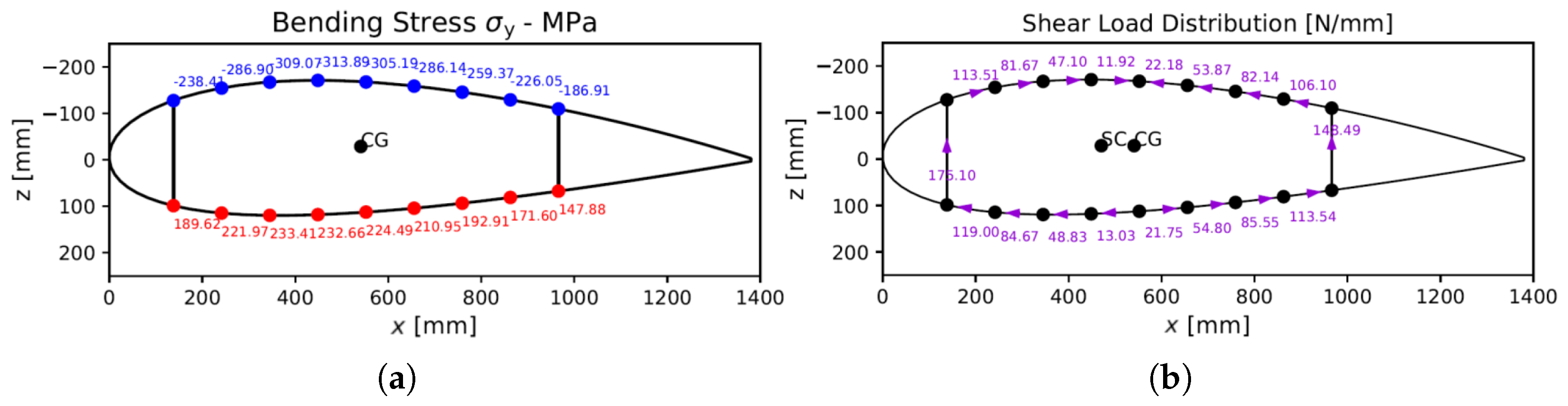
The acting force
is determined with the actual compressive stress due to bending
, calculated for the entire cross-section using Equation (
1) for a idealized wing box section, as illustrated in
Figure 7a. Similarly, the shear flow
over the wing box section is calculated using Equation (
2), as illustrated in
Figure 7b. In order to determine the most stressed representative cell, the interaction curve equation is evaluated for all possible combinations of the
ith stringer in the panel with the adjacent
jth skin pocket. Conservatively, the stiffened panel bay is sized based on the most critical representative cell within the entire bay. The critical failure index for combined buckling,
, is calculated considering the
calculated for every cell, such that:
4. Numerical Results
4.1. Metamodel Comparison
An investigation was conducted to compare the performance of the SVM algorithm with those of neural network architectures. SVMs and neural networks each consist of a set of methodologies, and several implementations are available in each category. The present study used the SVM implementation provided by the liquidSVM library [
29]. The multi-layer perceptron neural network (MLPNN) [
30] and radial basis function neural network (RBFNN) [
31] were used via the Stuttgart Neural Network Simulator [
32].
A set of sample points was randomly divided into two groups. The training set consisted of 700 points, and the testing set contained 300 observations. The metamodel was calibrated using the training set. Then the error was computed by using the information of the testing set.
Table 2 shows the metamodel error in mass estimation. The table columns display the following statistics: minimum, first quantile, median, mean, third quantile and maximum error values. The mean error of the SVM was
. The mean error of RBFNN was
. The mean error of MLPNN was
. The dispersion of the data followed a similar trend. SVM showed the best performance.
Table 3 shows the metamodel error in the feasibility estimate. The average error of the SVM metamodel was
, that of RBFNN metamodel was
and that of MLPNN was
. There are small differences among the errors of the metamodels, although SVM performed slightly better. The relatively high error levels confirm the fact that estimating the feasibility index is a challenging task.
In the present case, the neural network models used size = 300 as the number of units in the hidden layers and maxit = 1000 as the maximum iterations to be learned. On the other hand, SVM used the parameters max_gamma = 3125 and min_lambda = . All three methodologies support the selection of different kernel methods, and a myriad of parameter combinations. As a result, the comparison of metamodels can lead to different results if fine-tuning is performed for each methodology.
Due to the good results provided by the SVM methodology in the default configuration, it was used in the analysis that follows.
4.2. Data Analysis
The arrangement of SVM models as performance indices is detailed in the following. Three SVM models are proposed. The first model, named
, computes a mapping of the design vector
(Equation (
10)), the input data, to the mass of the structure
(Equation (
13)), the output data. The second model,
, computes a mapping of the design variables (input data) to the feasibility index
(Equation (
14)), the output data. The third model,
, performs a binary classification task, mapping the design variables (input data) to a feasibility classification
(Equation (
15), 0 for feasible designs and 1 for infeasible designs). The
liquidSVM library [
29] was used for numerical computation, as provided by the R software [
33]. In summary:
and
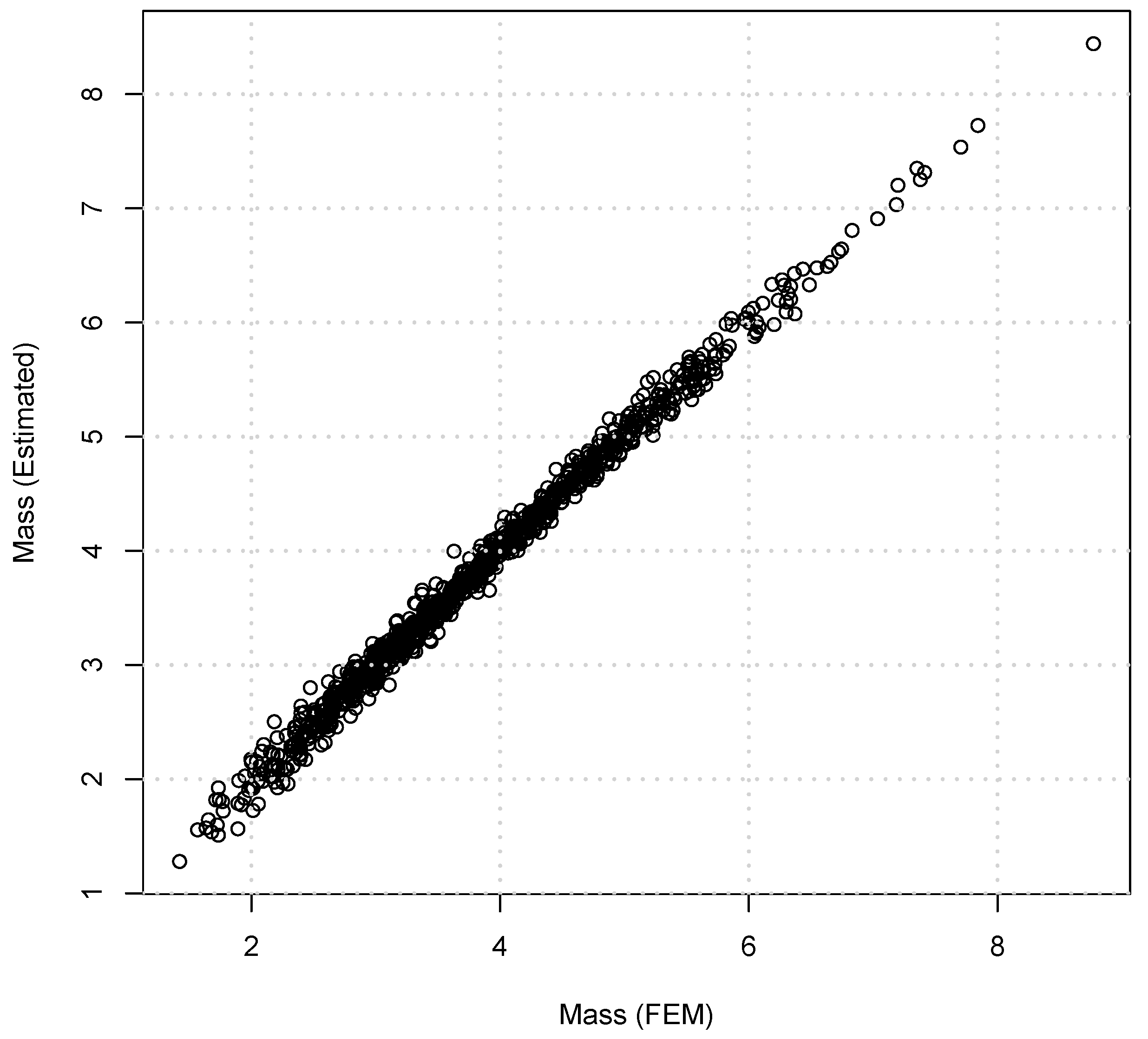
A comparison between the mass values obtained through FE evaluation and the estimates provide by the metamodel is presented in
Figure 10.
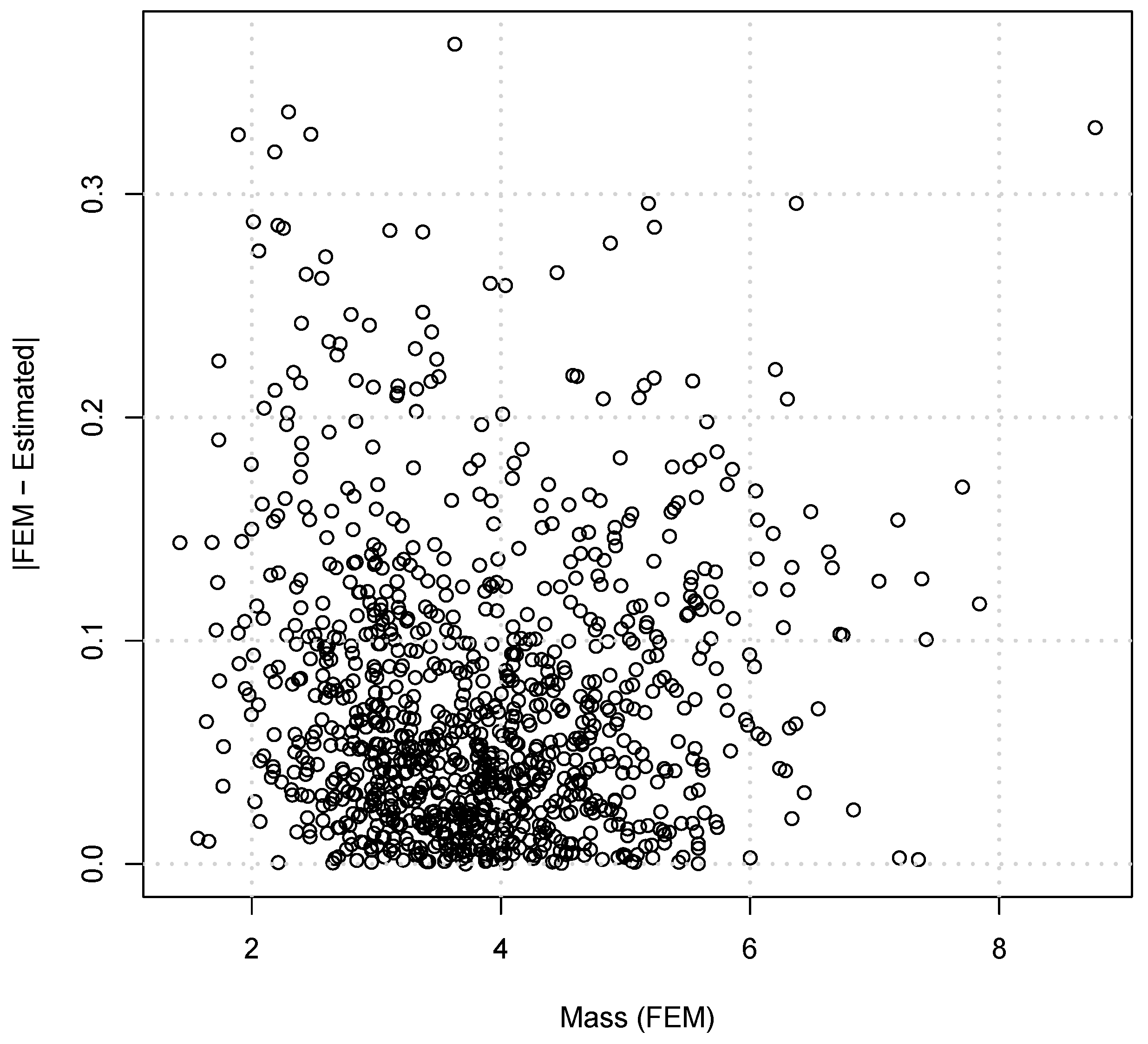
The absolute value of the difference between the mass computed by FE and the estimate is
and a comparison of error against mass is shown in
Figure 11. An histogram of the error
representing the difference between the mass computed by the FE model and the mass estimated by Equation (
13) is computed using Equation (
22), and shown in
Figure 12.
The results obtained from the FE and the estimates of the metamodel are similar, and the mass value was estimated with accuracy, as shown in
Figure 10.
Figure 13 shows a comparison between the feasibility values obtained through FE evaluations and the estimate provided by the metamodel.
The difference between the feasibility index computed by FE and the estimate is
whose absolute value is plotted against feasibility, as shown in
Figure 14.
The histogram of the error
, as per Equation (
23), is presented in
Figure 15.
Figure 13 shows that there is no clear trend between the design variables and the feasibility index; that is, some estimates are not representing the value obtained from FE with accuracy. This training phase required 1 second to calibrate the mass estimate and 218 s for the feasibility index. Given the poor correlation with the feasibility index, a more robust method is needed to classify the feasibility of the stiffened panel designs. A new feasibility classification is proposed to improve the success rate in obtaining optimal feasible designs. The step function (
for feasible designs and
for infeasible designs) was an effective improvement for the optimization formulation. The preference of mass or feasibility improvement is addressed by the parameter
. The multi-objective optimization formulation is written as
The design variables are box constrained (Equations (
11) and (
12)) by
Due to the discontinuous nature of the problem created mainly by the layout design variable
b, the computation of gradients is difficult, and the authors aimed to avoid gradient evaluations using finite differences. The aforementioned discontinuity leads to non-smooth behavior that fits better to an optimization method that does not require explicit gradient evaluations. It is estimated by a quadratic approximation on the BOBYQA algorithm [
34], which is adequate for the bound-constrained minimization in the absence of gradient information, and was used as implemented in the NLopt library [
35].
A discussion about the error between estimated and FE values follows.
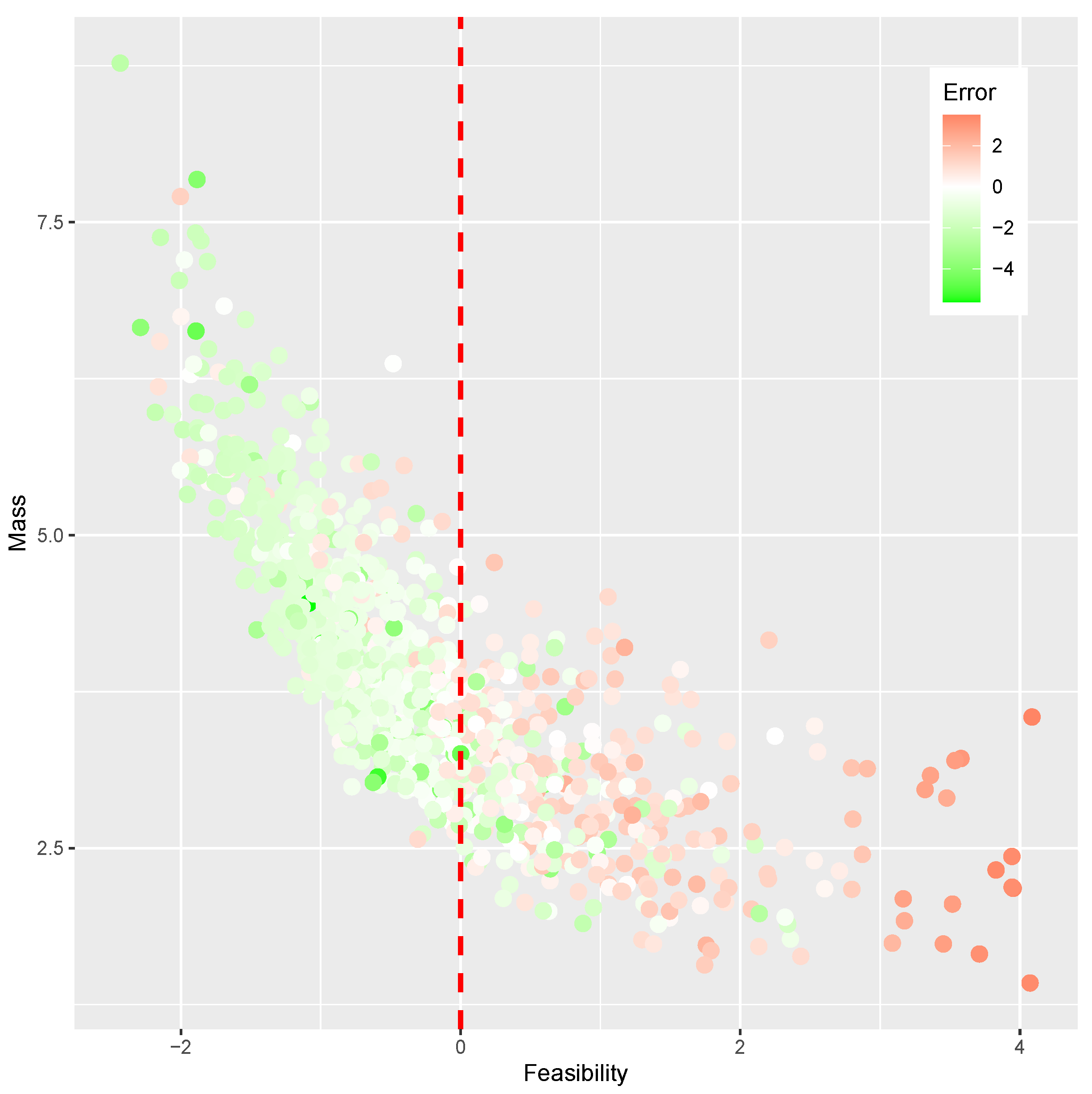
Figure 16 shows the mass against the feasibility index. Those values were obtained from DOE designs. The abscissa has valued of
and the ordinate represents the mass index
. The color palette represents the
error level. Designs with a small error are plotted in green, whereas designs with large errors are plotted in red. Larger errors were found in the range of infeasible designs
and in the range of high mass values
.
Figure 17 shows the error of the feasibility index. The abscissa has values of
, and the ordinate represents the mass index
. The error
is in green for small values and red for large values. Larger errors were found in the range of infeasible designs
, that is, where
.
The presence of an SVM-based classification index in the objective function enabled a deterministic optimization method to obtain the optimal design, yet with the ability to provide insight about the improvement obtained when mass and feasibility have different priorities, controlled by the weighting parameter . The change in priority of mass value against feasibility leads to distinct optimal designs, addressing the compromise of feasibility when the mass is reduced. As a result, insights are provided on how the change in design values affected the structural performance. The exploratory aspect of the design of experiments provides an overview about promising design values and a good initial guess for the optimization process.
4.3. Sensitivity of Parameters
Aiming to evaluate the effects of on mass and feasibility, the weighting parameter was investigated within the range . Furthermore, the effects of weighting feasibility index and feasibility classifier are discussed here.
The results of the numerical optimization (Equation (
24)) are now presented.
Table 4 shows the initial and optimal design values,
, changed. As
(Equation (
20)) was evaluated by means of a regression strategy and
(Equation (
21)) was evaluated by a classification strategy, some discrepancies may occur when comparing
and
(Equation (
24)). Optimal designs between lines 21 and 29 of
Table 4 show
and
. A contribution of the present study is the proposition of the classification index
as an objective. The classification index has proven effective at identifying feasible designs. Therefore, any design is considered truly feasible if
and
. Otherwise, the design is considered infeasible. The corresponding optimal designs are presented in
Table 5.
The SVM-based feasibility classifier indicates an infeasible state for 16 designs. The optimization was performed using real-valued design variables. The data obtained from the metamodel optimization indicate that the mean value of
is a robust value for the mass index. The 37 designs shown in
Table 5 were rounded to integer values to satisfy manufacturing constraints. The integer design values were then used to compute the mass and feasibility indices with the FE model, and the results are shown in
Figure 18.
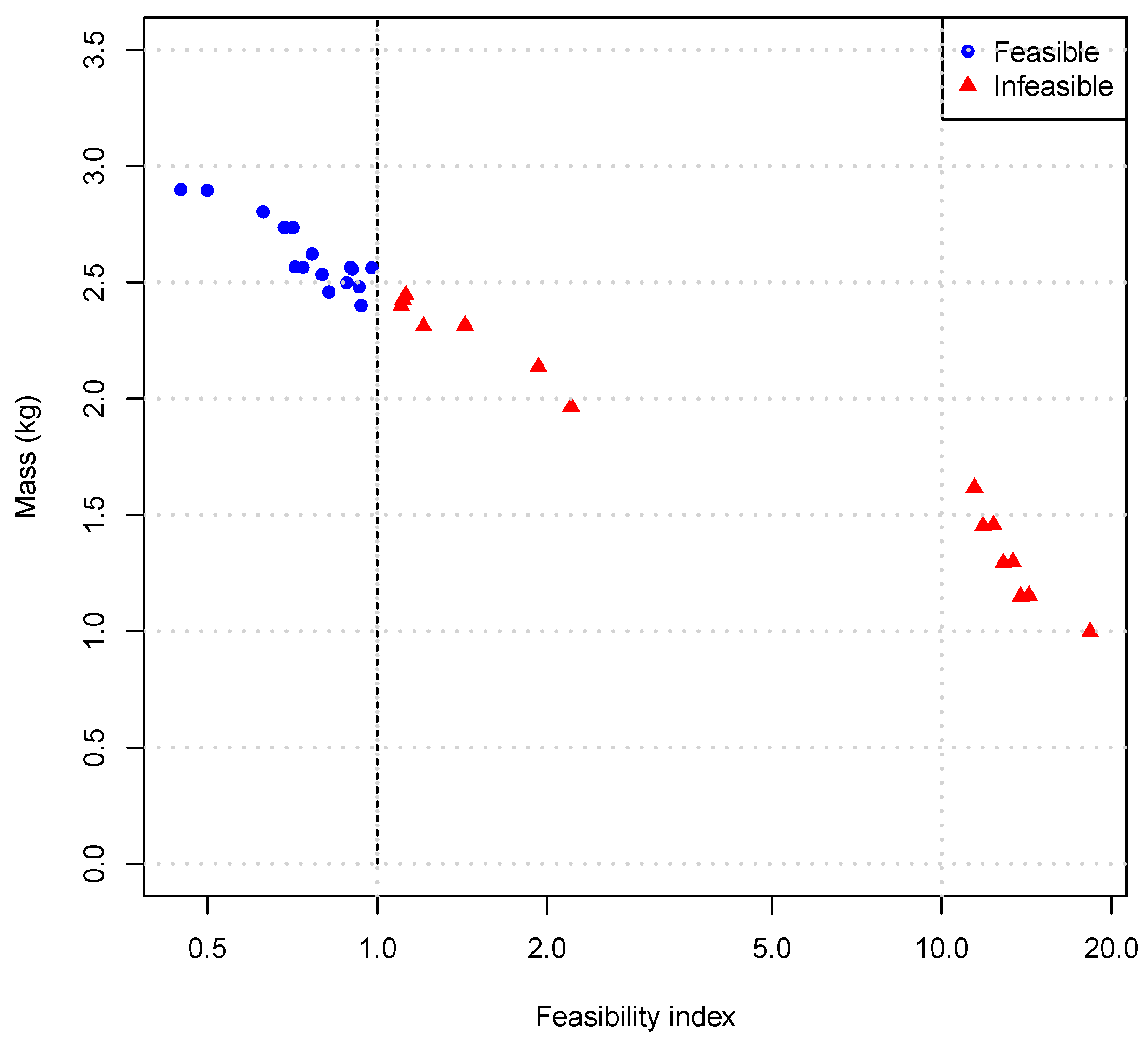
The mass index deviation is presented in
Figure 19. All points with mass values lower than
kg are infeasible from the structural perspective. Precise values are shown in
Table 4.
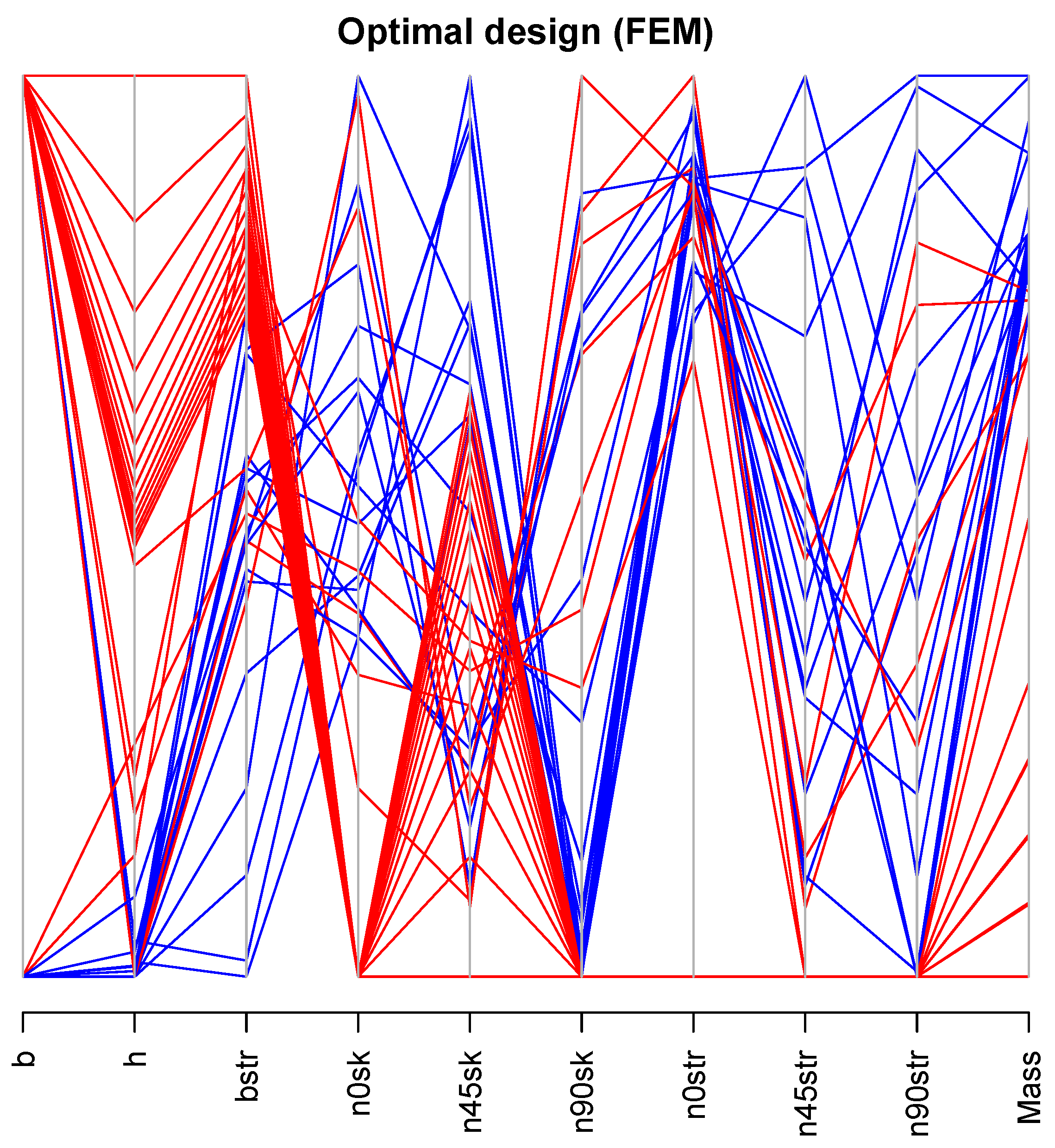
As shown in
Figure 20, several designs are concentrated in the range of lower
values. Designs with lower mass index are concentrated in the area of lower
and
values. Optimal feasible designs also have a trend around lower
h values. Several infeasible optimal designs are grouped in the range of lower values of
and
.
There is agreement between the optimal mass index found through the metamodeling and the values obtained by the FE model. The proposed workflow resulted in designs that are feasible and reduced the mass index. Furthermore, the optimization loop of several candidate designs gives insight into the sensitivity of the obtained solution. Distinct values of the parameter also resulted in designs with different masses. As expected, there is a clear compromise between mass reduction and infeasibility.
To investigate the sensitivity of the proposed optimization framework to the type of DOE, a second DOE was created using a more refined discretization of the
h and
design variable levels. Next, a new metamodel was trained, followed by optimization at different
values.
Figure 21 shows the optimal mass versus
parameter, with the mass computed using the FE model and the rounded-off variable values at the optimum designs obtained with the metamodel. The trade-off of mass and feasibility indices with
is shown in
Figure 22.
The comparison of
Figure 18 and
Figure 21 shows agreement of the optimal mass index in both cases. The mass and feasibility values had no significant change between the first and second DOEs, as also confirmed by the comparison of
Figure 22 and
Figure 23. As the mass index decreases, the feasibility index moves towards infeasibility. As a result, the lower the probability of obtaining a given mass value, the lower the chance of achieving feasible designs.
The exploratory capabilities of the current optimization framework allow browsing amongst the feasible options. The designer can choose a target feasibility index based on minimum margins of safety, mass or other requirements. This capability is illustrated in the Pareto fronts of
Figure 22 and
Figure 23. When there are no additional constraints, the feasible design that provides the minimum mass becomes a natural choice. Finally, the results of new FE evaluations can be added to the metamodel at any time to refine it in new or existing design regions.
In design problems with different numbers of variables, or for the current design problem with variables in different ranges, the new DOE is indirectly affected to handle the same errors presented here. One relevant factor to determine the necessary number of samples in the DOE is the ability of the metamodel to represent the interdependence of the design variables under investigation. More samples are required in cases where this interdependence becomes stronger, such as in structures where variable stiffness designs create a nonlinear coupling between the stiffness and geometric variables [
6,
21,
36,
37,
38,
39,
40]. A comprehensive discussion about the influence of the number of design variables is provided by Myers et al. [
41].
5. Conclusions
Herein was proposed a new method for optimal design of wing panels consisting of a framework that combines design of experiments, data interpolation, data classification and an optimization procedure. The methodology captures valuable information about the design space, identifying patterns and design trends discovered throughout the optimization workflow.
The exploitation of promising design regions was conducted using a deterministic optimization method. As there was no need to explicitly compute the gradient of the objective function, the method was able to navigate in a relative large area of the design space to explore the metamodel in the search for optimal alternatives.
A unique feature of the present contribution is the combination of regression and classification strategies in a multi-objective optimization formulation. Changes in the weighting parameter of the multi-objective functions proved to be an important feature for investigating the compromise between minimum mass and feasibility of the structure. Regression and classification indices in a multi-objective expression led to the effective exploration of the design space and avoided the premature convergence of the method.
The obtained Paretto fronts can be used to explicitly decide a target margin of safety for the designed panels, with a known influence on the obtained mass. In a case where no additional constraints exist and the target margin of safety is null, a natural choice for the selected design is the one with minimum mass in the entire feasible region.
Another challenging aspect of the present design problem that was well handled by the optimization framework is the simultaneous existence of discrete and continuous design variables. Usually, methods for exploring the space of integer solutions are computationally intensive and slower in convergence.
If information from new FE designs is available after the optimization cycle, the data obtained by the DOE phase can be supplemented with new information, and a new metamodeling and optimization cycle is started. It gives insights about how changes in design values influences the overall design indices.
Due to the applicability of the results found by the present analysis in the context of lightweight structures, the investigation of problems with greater complexity and more design variables is seen as the most important next step of the present research. The inclusion of design indices such as the b-factor in the initial post-buckling analyzes of imperfection-insensitive shells is also envisioned as an interesting application of the present optimization framework. There may be concurrency between designs aiming at negative b-factors and designs targeting higher linear buckling loads.


 ,
, 


