1. Introduction
Turbojet subsonic–sonic nozzles are devices that accelerate the hot gas incoming from the turbine by reducing the output area, generating more thrust. These devices are usually designed to optimally expand the gas at a particular operating point. The optimum expansion occurs when the
aeroengine exhaust gas static pressure matches the ambient pressure, maximizing the produced thrust [
1]. In the context of variable geometry, studies have shown that modifying the turbine nozzle can positively impact the fuel consumption [
2] and reduce the exhaust emissions [
3] when operating in off-design conditions. Hence, it is possible to conclude that the exhaust area must also be continuously adapted to the mission profile to improve the operating fuel efficiency.
Small-scale turbojets applications usually involve operating in environments with different sources of disturbances, from wind gusts and variations in the ambient conditions to more complex situations, such as variations in the effective payload [
4] that modify the required throttle turbojet setting. These turbojet disturbances translate into disturbances in both the nozzle input and nozzle output, since the turbojet thermal state directly affects the input nozzle gas-path properties [
5]. Maximizing the thrust production requires variable exhaust nozzles that reject the operating disturbances while optimally expanding the exhaust gas to the ambient conditions. Most of these difficulties can be assessed through suitable nozzle constriction and an adequate automatic control algorithm.
Although variable exhaust nozzles are highly attractive for military and some civilian applications, only limited information regarding nozzle automatic control is available. In the existing literature, several control schemes for variable exhaust nozzles are based on LQI control schemes [
6], which do not explicitly consider the possible sources of uncertainty and disturbances. Proper disturbance rejection consideration is a key element required to achieve reliable and efficient nozzle autonomy.
Turbojet control, on the other hand, has been a subject of interest of many researchers and different methods to overcome its difficulties have been developed. For instance, H
synthesis algorithms [
7], single neural adaptive propositional-integral-derivative
PID controllers [
8] and non-linear controllers based on a linear control-loop with an exogenous non-linearity [
4] have been developed to handle the process non-linearities. On the other hand, model uncertainty has been handled through
model predictive control in [
9,
10]. Control schemes focused on disturbance rejection have also been developed, such as those based on local optimum
PID controllers [
11] and those based on Active Disturbance Rejection Control
ADRC schemes [
12]. The
ADRC schemes showed promising capabilities to improve disturbance rejections in turbojets; however, a more realistic analysis on the disturbances is required. This shows an interesting area of opportunity to develop suitable variable exhaust nozzle controllers considering the particular difficulties of this process, which involve different sources of disturbances and model uncertainty.
This article presents a practical method combining the disturbance rejection capabilities of ADRC with the advantages of well-known classical control design techniques for variable exhaust nozzle control. Although in principle the application requires a non-linear controller due to the fundamental relationship among static pressure and gas velocity, the proposed design method allows designing the controller with linear control design techniques without compromising the non-linear stability condition. Moreover, this approach also allows designing the controller considering the desired robustness margins, model mismatch and input disturbances, ensuring closed-loop stability and safe operation. Finally, simulations performed with real-measured data from turbojet operation show that the proposed approach is able to increase the produced thrust when compared to a fixed-nozzle turbojet for the whole operating range in the presence of input disturbances.
2. Nozzle Modeling and Control Structure
Different aeroengine digital simulations have been developed based on AMESim [
13], Modelica [
13] and Simulink [
13,
14]; however, there are few reports dealing with variable exhaust nozzles with useful models from the control design point of view. Moreover, most of these models are dependent on nozzle geometry and variation mechanism. Thus, an appropriate model must be developed before attempting any control scheme. A useful and effective method for modeling aeroengines is the so called
first principle modeling approach, which departs from known physic fundamental laws to derive accurate dynamic representations [
15]. In this section, a novel variable exhaust nozzle model is derived from first principles and adapted for control design purposes.
Turbojet nozzles expand the incoming flow of the turbine output as shown in
Figure 1, where
is the nozzle input radius with area
and the input flow properties are given by its temperature
, pressure
and velocity
. The nozzle increases the output speed
and thus reduces the exhaust gas pressure
and temperature
. If the mass flow holds constant, the only means for actively modifying the flow speed is to increase or reduce the output area
by modifying constriction angle
. Whereas traditional aeroengine controllers normally regulate shaft-speed by modifying the input fuel flow [
16], variable exhaust nozzles effectively introduce an additional control input, introducing the possibility of implementing a secondary control loop.
Since the velocity varies within a bounded neighborhood of operating points near the design point, the density can be assumed as steady and constant in space. This implies that:
where
u is the advective field. This results in the following momentum and energy,
e, equations:
where
V is the flow velocity,
P is the pressure and
its density.
Considering the nozzle configuration and the variables defined in
Figure 1, then the mass conservation integral for incompressible flow yields:
where
is the control surface contour.
Recalling that the nozzle inlet area
remains constant it is possible to obtain the change of the nozzle velocity with respect to time by calculating the time derivative to both sides of Equation (
4), which yields:
The turbine output velocity can be approximated through the mass conservation principle if the gas path properties (i.e., turbine output pressure,
and turbine output pressure
) are known. That is:
where
is the turbine mass flow and
R is the universal gas constant. Thus, the nozzle inlet velocity derivative with respect to time is:
Therefore, the nozzle inlet velocity change can be written as:
If the nozzle length
l is fixed, then the output area becomes:
and the nozzle output area change with respect to time:
Recalling Equation (
5), the nozzle dynamic behavior is described as:
2.1. Model Linearization
Then, the linearized velocity
is described through:
where circumflex character indicates the deviation from the equilibrium conditions
, i.e.,
. The elements of Equation (
12) are computed through:
with
being the gas-path derivatives:
Considering that the linearization corresponds to an arbitrary equilibrium point so that
, Equation (
12) yields:
where
. Transforming Equation (
23) into a Laplace domain yields:
where
are the constant coefficients of the linear approximation (
23).
Since only the constriction angle can be directly manipulated, all the remaining elements of Equation (
25) are considered to be input disturbances to the process. That is:
where
is the Laplace transform of the perturbation signal.
2.2. Model Uncertainty Quantification
Equation (
25) shows that the nozzle input/output dynamics depend mainly on
. Thus, recalling Equation (
20), for feedback control, the main sources of plant parametric uncertainty are:
The turbojet thermal state in which the model is linearized. The linearization point within the turbojet equilibrium manifold plays an important role. Its effects are translated into the equilibrium output speed, . This represents the turbojet exhaust gas speed at equilibrium conditions in a given thermal state with a fixed nozzle.
The equilibrium constriction angle, . This is the constriction angle in which the model is linearized.
To reduce the effects of this parametric uncertainty, a family of model parameters can be computed for each possible operating condition and nozzle constriction configuration. This is presented in
Figure 2, which shows the resulting values of
from Equation (
25) with respect of the turbojet operating condition and nozzle constriction angle.
If a nominal model (
25) is obtained at the operating point
260 m/s and
, according to the turbojet operating limits, the uncertainty corresponding to
is bounded such that
with
,
and
the nominal value.
2.3. Control Structure
The control objective is to maximize the thrust
T generation for a given throttle setting and environmental conditions. The thrust is defined through [
17,
18]:
where
represents the ambient pressure,
the inlet mass flow and
the free-stream wind speed. Therefore, the optimal exit pressure for a maximum thrust is
. Thus, it is convenient to define a pressure-based control error
as follows:
Figure 3 presents an ideal pressure-based control loop considering the optimal expansion of the exhaust gas. However, directly controlling the static pressure without acting through the dynamic pressure
may be too complicated in a practical setup.
Alternatively, it is possible to complement the exhaust gas velocity model (
11) with an output mapping function
that relates the flow velocity and the flow dynamic pressure. Considering this arrangement, the Wiener-like structure of
Figure 4 is obtained where
and:
The total pressure
is related to the static
P and dynamic pressure
through:
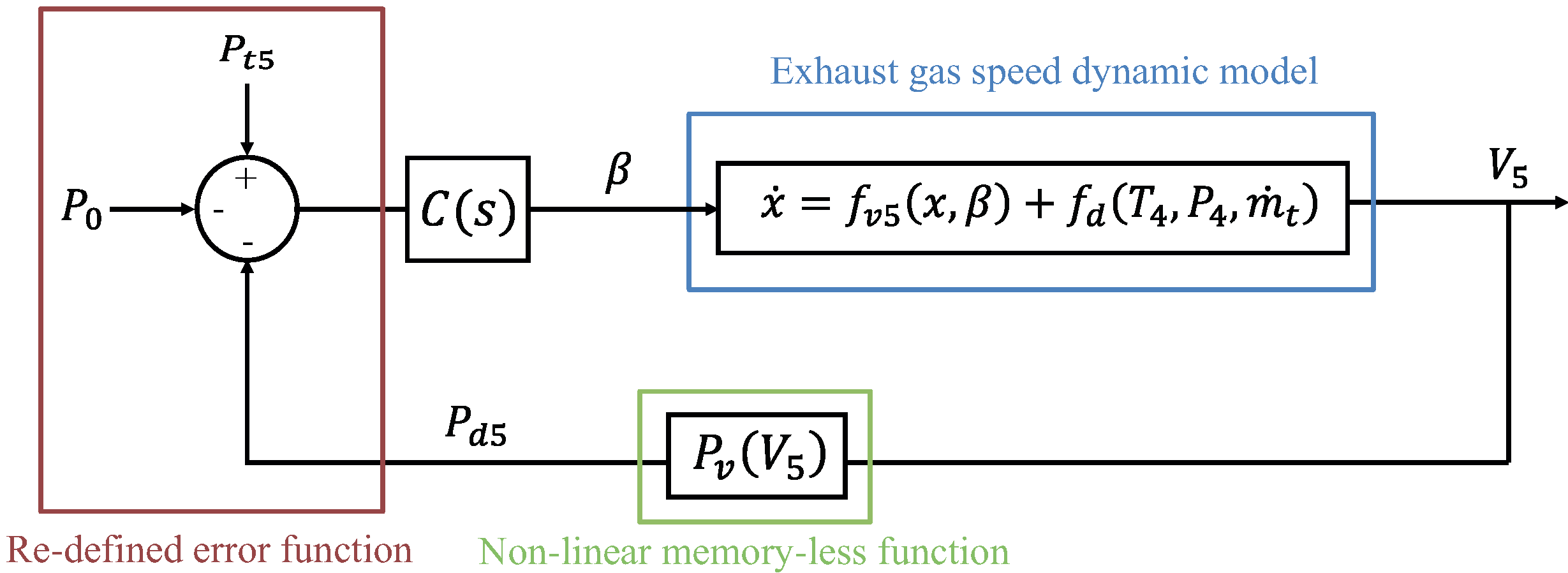
. If this relationship holds, combining the Wiener model of
Figure 4 into the proposed control structure of
Figure 3 yields the novel control structure of
Figure 5. This scheme closes the exhaust gas velocity control loop through the constriction angle, while maintaining the effects of the turbojet operation configuration (i.e.,
) as input disturbances. The advantage of this representation is that the controller can be designed using the exhaust gas velocity linear model (
25) if adequate disturbance rejection and uncertainty specifications are considered. Note that the error function has now been re-defined to maintain a negative feedback and to suit the velocity-based control scheme, yielding:
The physical interpretation of the involved variables shows that the non-linear static function
is a polynomial that associates the air speed to the dynamic pressure, which is a well know flow property [
17,
18]:
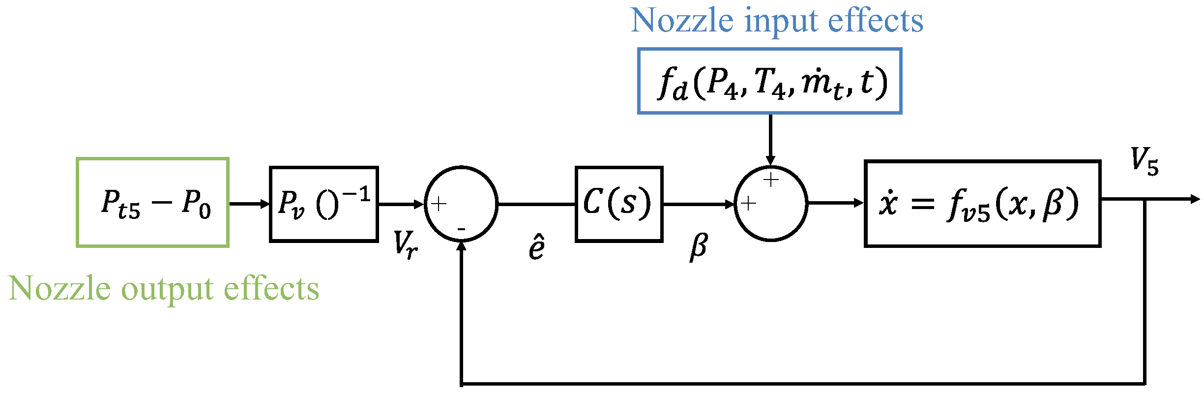
Moreover, a key advantage of this structure is that the non-linear element can be inverted to realize a linear exhaust air-speed control loop, allowing to implement classical control design tools. Inverting this polynomial determines a reference air-speed,
, in terms of the turbojet output pressure (strongly related to the throttle settings) and the environmental pressure. This reference air-speed describes the required air-speed to optimally expand the output nozzle flow:
From a practical standpoint, the turbojet inlet mass flow, compressor output pressure and temperature are influenced by the throttle setting and environmental conditions. The variations of these variables are external to the nozzle and are thus considered as disturbances to the nozzle dynamics. The controller aim is to reject its influence into the output air-speed. Considering the influence of each variable into the airspeed yields the control scheme of
Figure 6.
This control structure allows minimizing the error among the measured exhaust gas velocity and the velocity required to completely expand the exhaust gas, while handling the input disturbances caused by the turbojet operation (changes in the thermal state). The previous discussion during the modeling and control structure design shows that it is fundamental for a nozzle controller to successfully reject disturbances.
3. Robust Nozzle Control
In recent years, the Active Disturbance Rejection Control (
ADRC) has emerged to fit the necessity of controllers that succeed in applications that demand high accuracy, robustness and simplicity. This approach combines the simplicity and applicability of known classical control methods with a model-based approach. For instance, the resulting controllers of the linear case of the
ARDC are compatible with most frequency-response based analyses [
19], allowing its evaluation in terms of bandwidth and stability margins.
The main difference from other model-based approaches that assume canonical models of the actual process dynamics, such as model predictive control or embedded model control, is that in
ARDC the model is not dependent upon accurate mathematical modeling of the plant [
20]. The central idea of these controllers is to use an Extended State Observer (
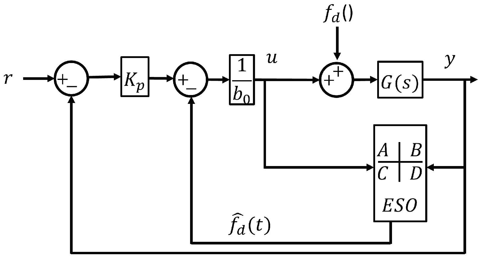
ESO) to estimate the process disturbances, parameter variations and uncertainties in real time. This is presented in
Figure 7, for a first-order Linear Active Disturbance Rejection Control (
LADRC). Although at first glance, the
LADRC is simple, it provides remarkable robustness to variations in the process dynamics and external disturbances [
21].
LADRC can be developed by considering a state space control with disturbance estimation and compensation based on the internal model principle. Thus, showing additional compatibility with analysis and design tools based on state space representations.
3.1. The concept of Linear Active Disturbance Rejection
A basic derivation of
LADRC is shown as follows. Consider the first order plant:
where
y is the system output,
w the process disturbances,
u the input and
b a constant. Then, it is possible to define that
,
being the known part of
b obtained through the modeling process and
the uncertainty in this parameter. Thus, the combination of
can be defined as a generalized disturbance
so that:
If the disturbance
can be estimated and compensated, the system is reduced from a first order to a single integrator plant with a scaling factor
. The estimation of
can be achieved by introducing an
ESO for the following system:
with
and
.
The
ESO of Equation (
35) was augmented to include the additional state
, since it can only be reconstructed using the process input,
, and output,
. In
LADRC, a Luenberger observer can be used to estimate the state:
where
and
are estimations of
y and
correspondingly. If using bandwidth parameterization, the observer gain vector
can be chosen to locate its eigenvalues at the desired observer bandwidth [
20],
:
With a well-tuned observer (i.e., if the
ESO dynamics are fast enough to follow the disturbances) the estimated disturbance
can be used to implement the actual disturbance rejection controller:
This reduces the plant to an integral process:
If the control law is defined as:
the controller acts on
rather than
, making
K an integral controller gain. Thus,
K can be tuned according to the desired settling time
:
3.2. LADRC+Classical Controllers
Although being practical and useful for processes that operate in environments with high level of disturbances, the
LADRC does not provide a priori insight on the frequency-domain characteristics of the resulting controlled plant. That is, classical design elements such as bandwidth, sensitivity, phase margins, gain margins and sensor noise rejection cannot be used directly as a source of information for the controller design.
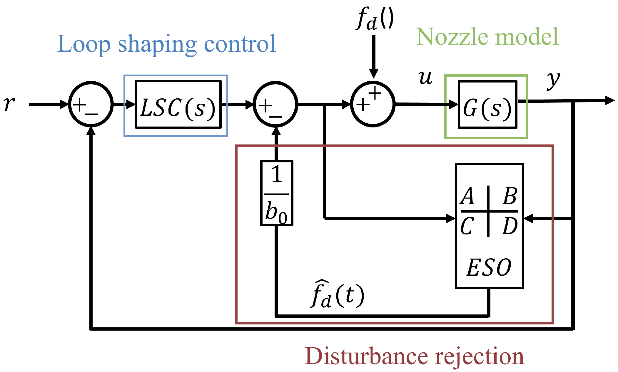
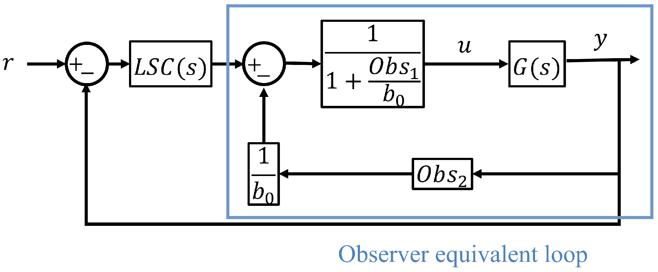
Figure 8 presents a novel control scheme achieved by combining a loop-shaping controller (
LSC) with the estimation of the disturbance from the
LADRC. This approach allows designing a classical controller for the known process dynamics considering key frequency-domain specifications, while taking advantage of the
LADRC disturbance rejection capabilities.
In order to elucidate the effects of each controller in the closed-loop dynamics, as follows an alternative representation is derived by dividing the
ESO into its respective individual transfer functions. This is presented in
Figure 9.
In absence of disturbances, the closed-loop response is given by:
with the observer equivalent loop,
, being:
Correspondingly, from (
36) and (
37), the equivalent observer transfer functions parameterized to
and
can be shown to be:
Substituting Equations (
44) and (
45) into Equation (
43) yields:
This implies that, in the absence of disturbances (i.e.,
) the estimated disturbance
will also tend to 0. Thus, the closed loop will defined by the plant and
LSC if no input perturbation is present, that is:
Equation (
47) shows that
LADRC is separable from any feedback controller if only the disturbance rejection element is used. Thus, the effects of the
LADRC are only visible when considering the input disturbance and noise sensitivity functions.
4. Control Design and Assessment
Four controllers are designed considering Equation (
25). The evaluated controllers are a proportional-integral
control, a single loop shaping control
, a linear active disturbance rejection control
and a combined
scheme. This section includes the controller evaluation within time-domain and frequency-domain frameworks.
4.1. Control Objectives
The control specifications are aimed at following common aeronautical certifications for high performance applications, including air-to-air and air-to-ground tracking as well refueling and close formation flying for small or unmanned aerial vehicles. Being able to introduce these standard classical specifications is one of the advantages of the proposed approach, making the resulting controllers compatible with most certifications. The specifications are summarized as follows:
Settling time smaller than 5 s [
22];
Bandwidth
range of 6 rad/s to 11 rad/s [
23];
Minimum 6 B gain margins Gm [
24];
Minimum of 45 deg phase margin Pm [
24].
4.2. Control Design
The controllers are designed as follows:
- 1.
Proportional-Integral control
PID controllers are an important industrial standard [
25] and are thus, added into this evaluation. In the absence of disturbances, the dynamic model (
25) yields a zero-order representation of the nozzle dynamics. Thus, the controller in series with the plant is [
26]:
Since the integrator provides a phase of −90 deg, the gain margin is infinite. Thus, it is not considered in this analysis. The magnitude equation in a frequency-domain is:
Since the amplitude at the bandwidth frequency
is approximately 1, Equation (
49) yields:
The corresponding closed-loop response and settling time are given by:
Thereafter, the parameters of Equations (
50) and (
52) are computed through numerical optimization to find the controller configuration that provides a settling time
with a bandwidth
. The resulting
PI controller is:
- 2.
Loop shaping control
A similar process is carried out for the
LSC, which is proposed as a lead/lag compensator. The
LSC in series with the plant is [
27,
28]:
Here, the objective is to compute the
LSC gain
, zero location
and pole location
. Following the analysis performed for the
PI controller, the corresponding phase margin (
55), gain at the bandwidth frequency (
56) and settling time (
57) equations for the
LSC are given by:
Moreover, it is a good practice for loop shaping compensators to locate the poles equally distant from the banwidth in the frequency plane. Thus, the following design rule is added:
Parameter optimization of Equations (
55)–(
58) yields the following lead-lag compensator:
- 3.
Linear Active Disturbance Rejection Control
The parameters of this controller are computed according to the process described in
Section 3.1. The settling time is defined such that it provides a similar response time than the
PI controller. To achieve a settling time of 0.5 s, the gain
K is:
Since the desired control bandwidth is about 10 rad/s, the observer bandwidth is located at
. Using Equation (
37), the corresponding Luenberger observer gain is:
- 4.
LADRC + LSC design
It was demonstrated in
Section 3.2 that the
LADRC and
LSC can be designed separately, if only the disturbance estimation of the
LADRC is used. Thus, this model combines the previously developed
LSC (
59) and a
LADRC with the parameters (
60) and (
61) within the structure of
Figure 8.
4.3. Time-Domain Analysis
Typical aeronautical control applications involve operating in environments with frequent disturbances and sensor noise from the wind-speed measurements. These are analyzed individually through the following simulations.
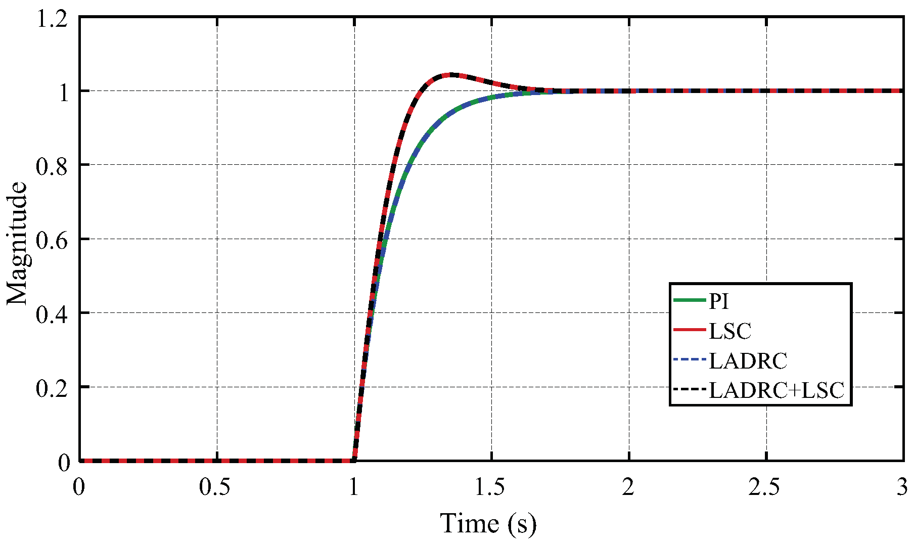
Figure 10 shows the step response of the controlled plant with each controller. It is possible to conclude that, in absence of noise and disturbances, the
LADRC provides a similar response than a classic
PI controller. The similitude among the
LSC and the
LADRC + LSC is not surprising, since the closed-loop robustness and stability are determined solely by the
LSC.
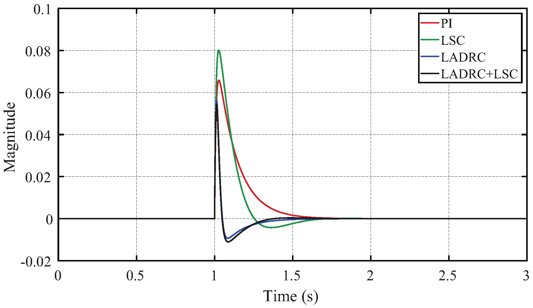
The disturbance rejection capabilities of the controllers are evaluated in the simulation of
Figure 11. The
LSC provides a faster disturbance rejection than the
PI, at the cost of a higher overshoot. The
PI controller follows a more conservative response with a slow disturbance rejection. The
LADRC and the
LADRC + LSC are the fastest and effectively cancel the disturbance effects with little overshoot. It is remarkable that the
LADRC + LSC maintains the effects of the
LADRC disturbance rejection capabilities.
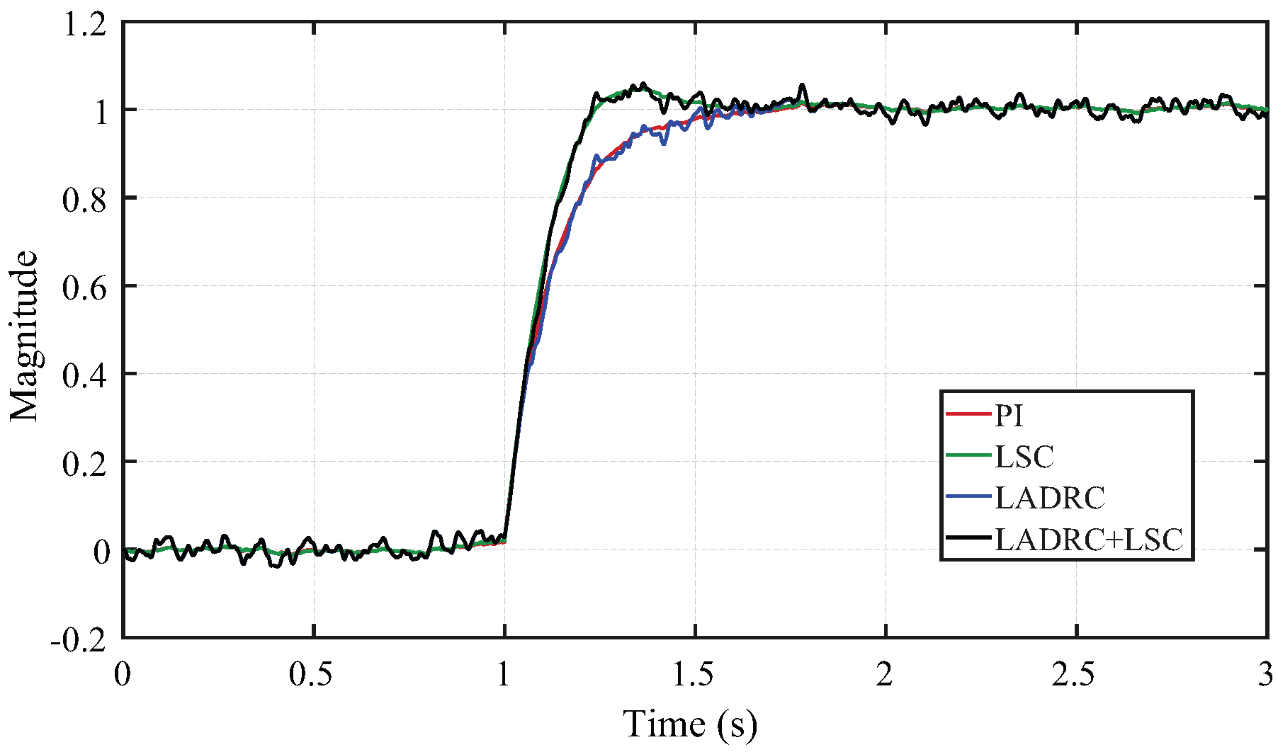
Figure 12 shows the unit-step response of the controllers with simulated sensor noise. Both the
LSC and
PI reject the noise effectively, while the sensor noise mostly affects the
LADR-based controllers. This is more evident when analyzing the frequency-domain response of these controllers shown in the next section.
4.4. Frequency-Domain Analysis
This section studies the frequency-domain response of the controllers. The frequency-domain analysis of the LADRC is calculated by reducing the system into a set of transfer functions, after replacing the ESO by the respective transfer functions for each channel. The PI and the LSC were computed such that the bandwidth was located at a specific value. This is important when handling the bandwidth limits stated by the sensors and actuators. The LADRC; however, automatically allocates the bandwidth and presents a challenge to design the controller when considering this parameter. Thus, rendering its application impractical for some applications. This problem can be reduced when using the LADRC + LSC configuration.
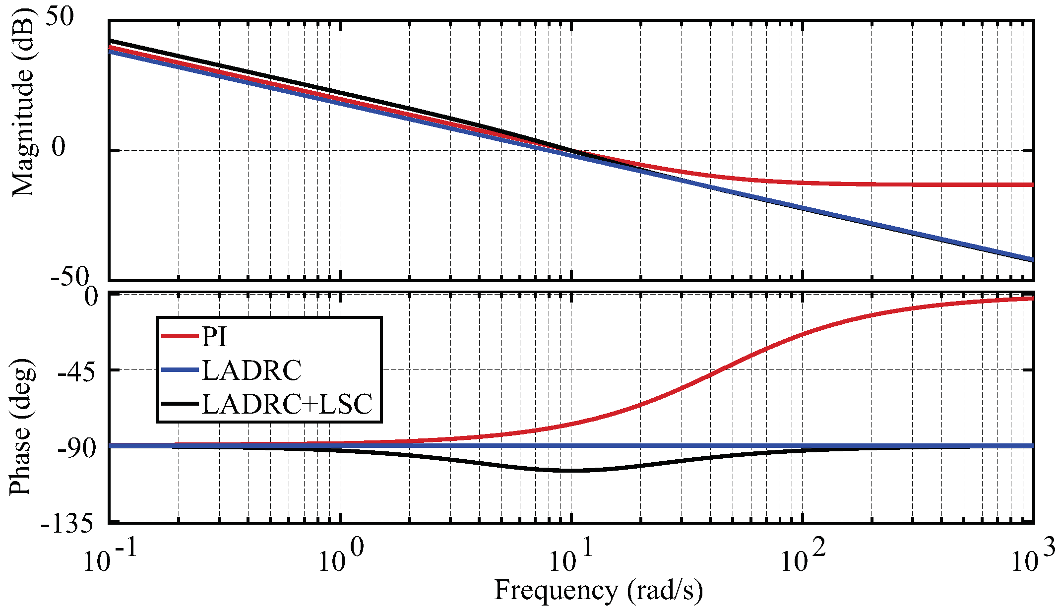
Table 1 shows the gain margin, phase margin and bandwidth of the resulting plant + controllers, while
Figure 13 shows their open loop frequency response. Overall, most controllers succeed with the stated control objectives.
4.5. Interaction of LSC and LSC + LADRC
As stated in
Section 3.2, the difference among the
LSC and the
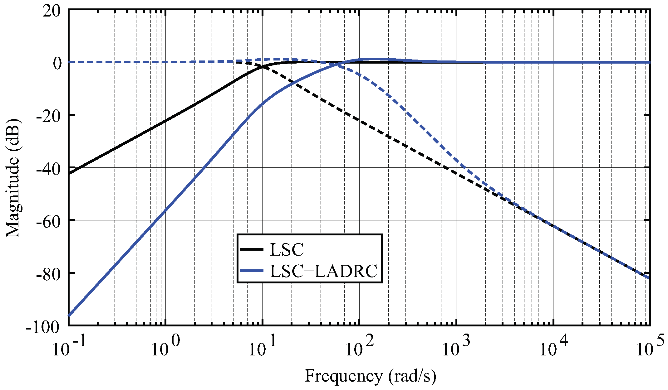
LADRC + LSC schemes can be observed better in the input disturbance and noise sensitivity functions, presented in
Figure 14. The addition of the
LADRC greatly improves the disturbance sensitivity in low frequencies, at the cost of increased noise sensitivity. It is notable that the increased perturbation rejection of the
LADRC + LSC (over 15 dB around the bandwidth compared with the
LSC) is achieved without increasing the closed loop bandwidth. This shows that the
LADRC + LSC has remarkable perturbation rejection properties.
The previous analysis suggests that LADRC + LSC schemes are useful for applications with (i) uncertainties in the plant dynamics, (ii) changing environments with frequent disturbances and (iii) availability of measurements with a sufficiently low noise level.
4.6. Stability Evaluation with the Non-Linear Static Gain Uncertainty
Since the nozzle process inherently faces different sources uncertainties, it is important to account for its effects with respect to the developed models [
29]. The uncertainties can be introduced by the incompressibility approximation, possible measurement error and model mismatches caused by the linear approximation.
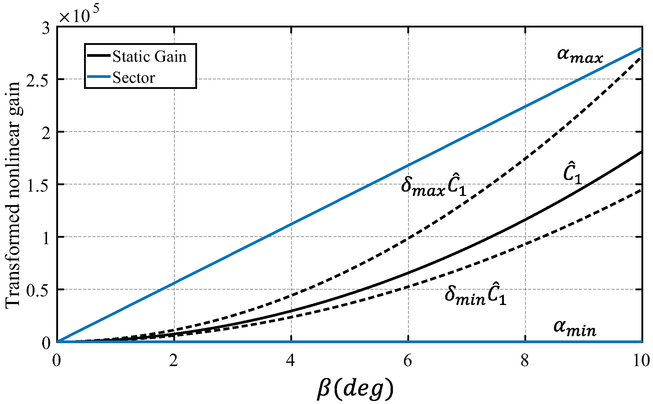
Figure 15 presents the uncertainty effects in the transformed-model non-linear gain. Recalling
Figure 2, the slight differences from the nominal gain to the model maximum and minimum gains are bounded by the sector limits defined by the slopes
and
.
With this context in mind, the closed loop stability is evaluated with the best-suited controller for this application among the evaluated control schemes, the
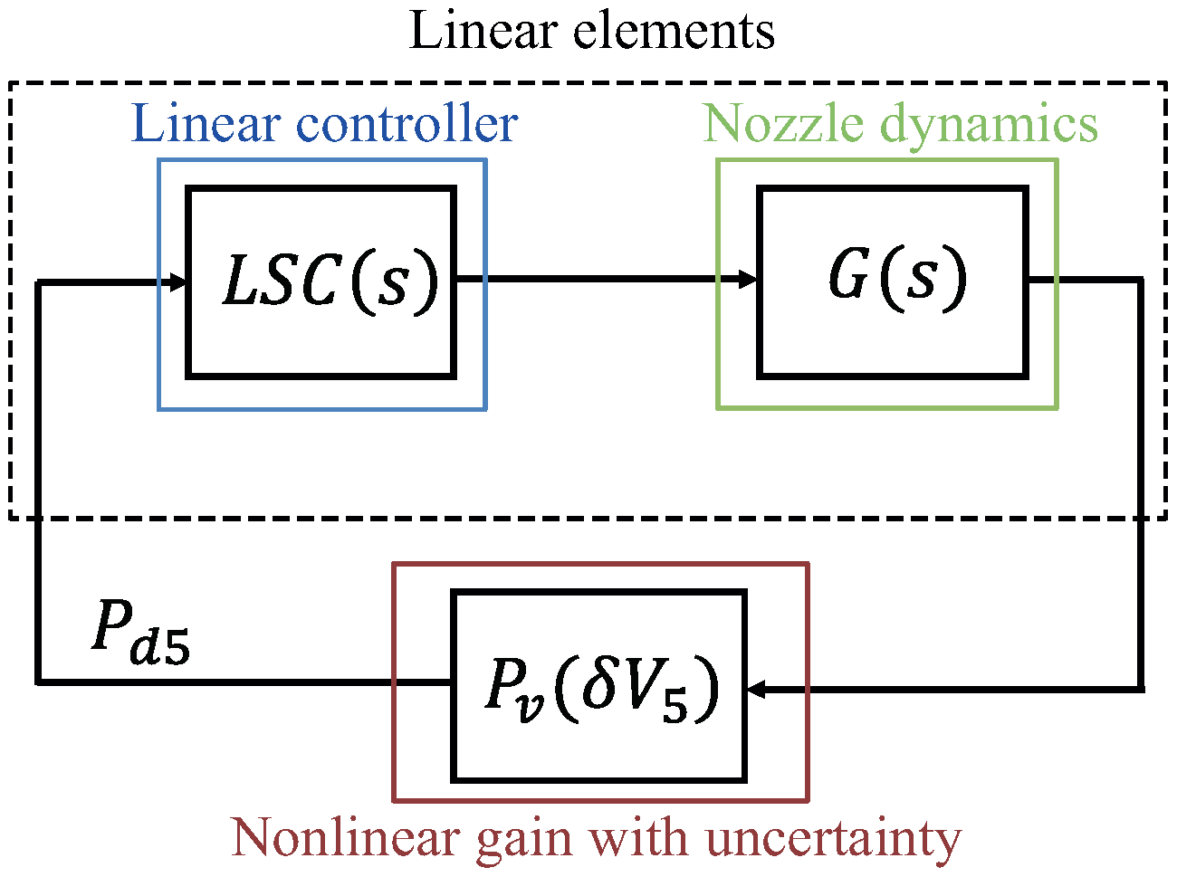
LADRC + LSC. The uncertainty caused by the mismatches among the linear approximation and the non-linear model may present adverse effects in the stability of the system. Thus, prior to its application, it is important to evaluate the resulting controllers with the non-linear static gain uncertainty. This is achieved by transforming
Figure 6 into the structure of
Figure 16. This structure includes the linearization uncertainty within the static pressure non-linear gain, yielding an autonomous representation that allows analyzing the model robustness properties with absolute stability tools [
30].
The transformed non-linear gain of
Figure 15 lies within a sector that includes the effects of the linearization uncertainty. Thus, the linear elements of the autonomous system representation can be analyzed with sufficient stability conditions [
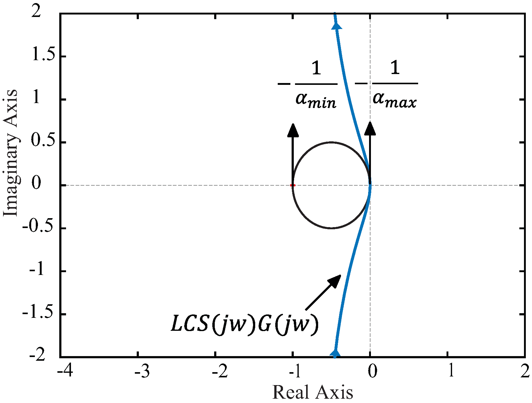
31]. A practical test for asymptotic stability is the
circle criterion, as presented in
Figure 17. The Nyquist path for the linear elements (i.e.,
) does not encircle nor touch the circle defined by
and
. This shows that the exhaust gas velocity loop is asymptotically stable for the analyzed operating range.
5. Case of Study: Exhaust Nozzle Area Control
The resulting
LADRC + LSC is evaluated with real operational data measured from turbojet operation and the non-linear simulation of the variable exhaust nozzle of Equation (
11). The data was measured with the SR-30 turbojet test bench, which has been previously used to perform thermodynamic and data-mining analyses [
5]. This test-bench allows measuring the generated thrust, shaft speed, fuel flow and gas-path properties at the input and output of each component.
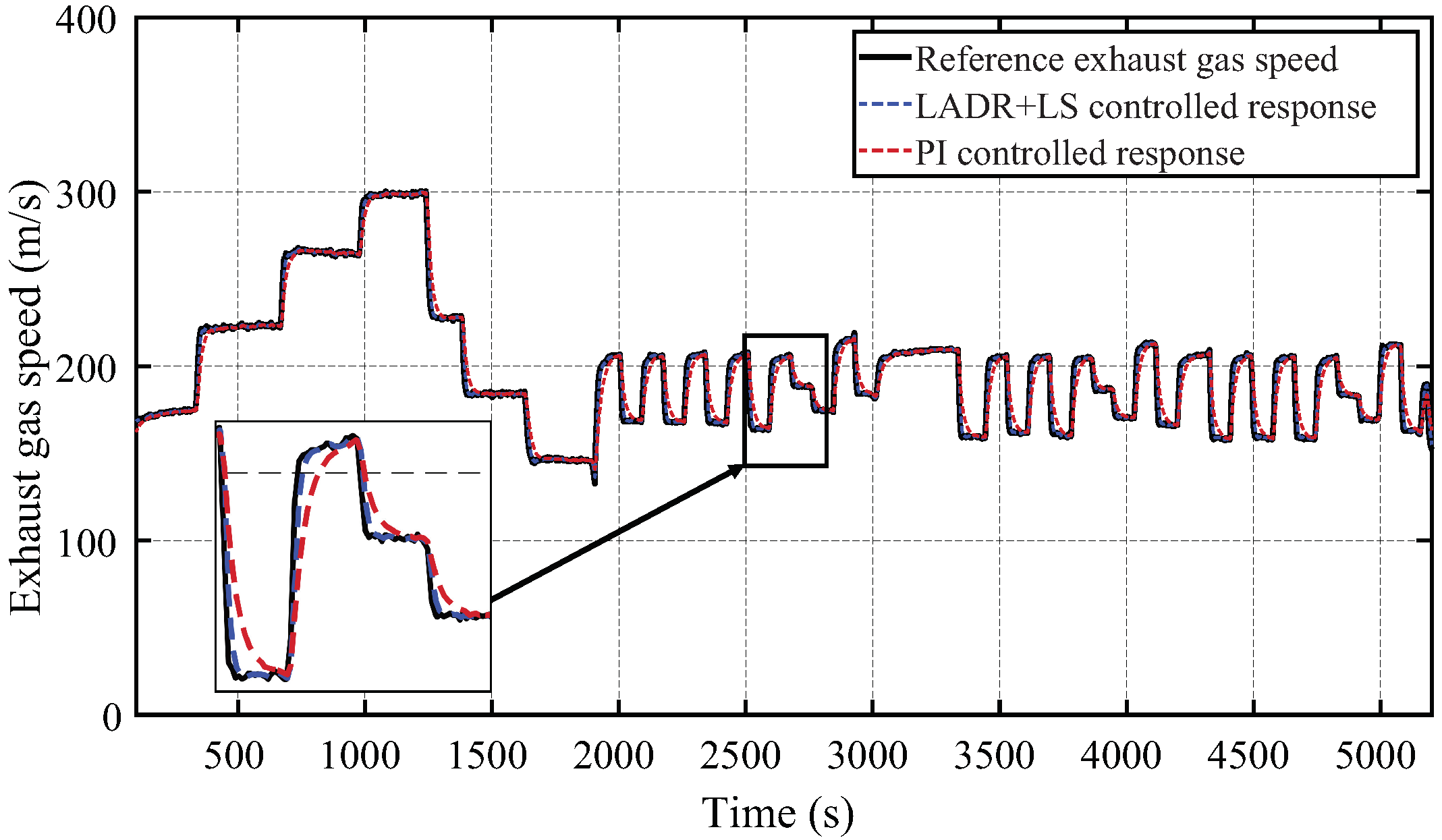
Figure 18 presents the reference tracking of the objective exhaust gas speed required to maximize the thrust of the SR-30 turbojet. The controlled system effectively expands the exhaust gas in every tested operating condition, considering the non-linear dynamic nozzle model (
11).
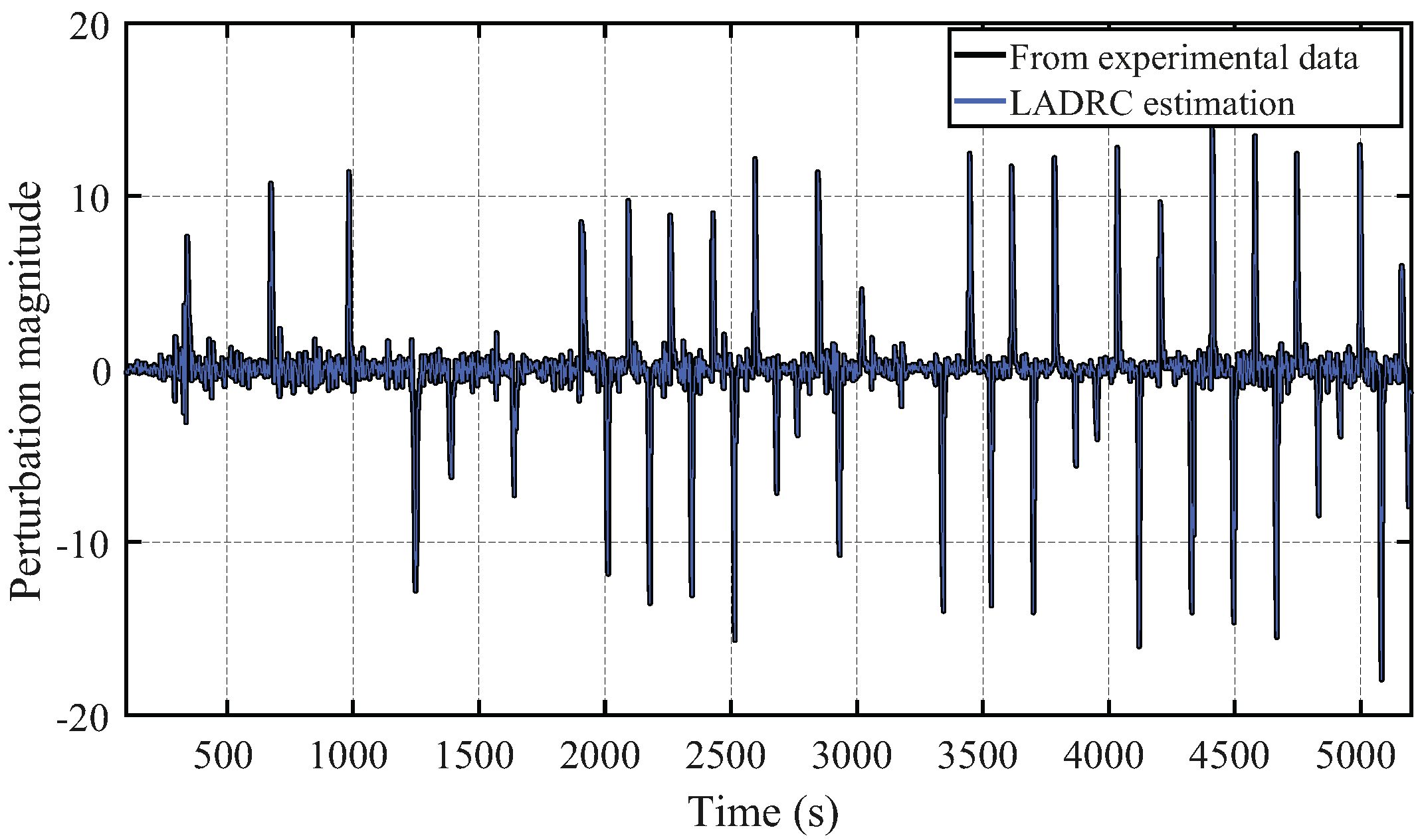
On the other hand, the
ESO designed of the
LADRC scheme effectively estimates the disturbances caused by the turbojet thermal state changes (i.e., throttle setting changes). This is shown in
Figure 19, where the estimation closely follows the input disturbance
. This disturbance is caused by changes in the aeroengine thermal state. That is, when the fuel flow is increased or decreased, the corresponding changes in the gas path variables (
and
) and mass flow affect the nozzle input gas speed. The combination of the effects of each individual variable into the nozzle input gas speed are encompassed in the disturbance
.
6. Discussions
This article shows that it is feasible to develop a suitable nozzle control considering the most common issues inherent to this process. As summary, these issues involve:
Developing comprehensive mathematical representations to capture the nozzle dynamics and adapting them for efficient controller design.
Elucidating the possible disturbance sources that affect the nozzle performance.
Evaluating the resulting model in terms of parametric uncertainty.
Structuring a suitable closed-loop control scheme that considers the nozzle area manipulation and its effects into the exhaust gas flow.
Achieving a control that specifically handles the possible nozzle disturbances and uncertainties observed during the modeling process.
Evaluating the resulting closed-loop scheme in terms of robustness margins and classical performance metrics.
Determine the non-linear stability condition of the closed loop system with respect to the process uncertainty.
The resulting control scheme allows maximizing the produced thrust with respect to the environmental and total exhaust gas properties. This is a novel approach that, according to a comprehensive literature review and the best knowledge of the authors, has not been presented yet in any public academic database.
The proposed combination of a LSC with an LADRC yields a practical method for controller design with improved disturbance rejection characteristics. The main advantages are that the LSC can be designed considering the control objectives in terms of classical stability and performance margins, bandwidth and additional criteria that the designer considers appropriate (such as loop attenuation at high-frequency). Thereafter, the LADRC can be designed with respect to the LSC bandwidth. However, it is important to consider the resulting trade-off among the improved disturbance rejection characteristics of the system and the resulting noise sensitivity. Nonetheless, the presented procedure allows a clear evaluation of this compromise.
When considering the uncertainty caused by the linearization, the resulting
LSC + LADRC can maintain the desired performance properties, while classical controllers struggle when handling the nozzle non-linear dynamics. This is shown in
Figure 18, where the
PI controller provides a slower response when compared to the the
LSC + LADRC, which follows more closely the desired exhaust gas speed. It should be noted that the differences among both control schemes (i.e.,
PI and
LSC + LADRC) are reduced if the linear engine model is used for the simulation. This shows that the improvements observed in the
LSC + LADRC scheme are due to it successfully rejecting engine non-linearities.
6.1. Thrust Augmentation
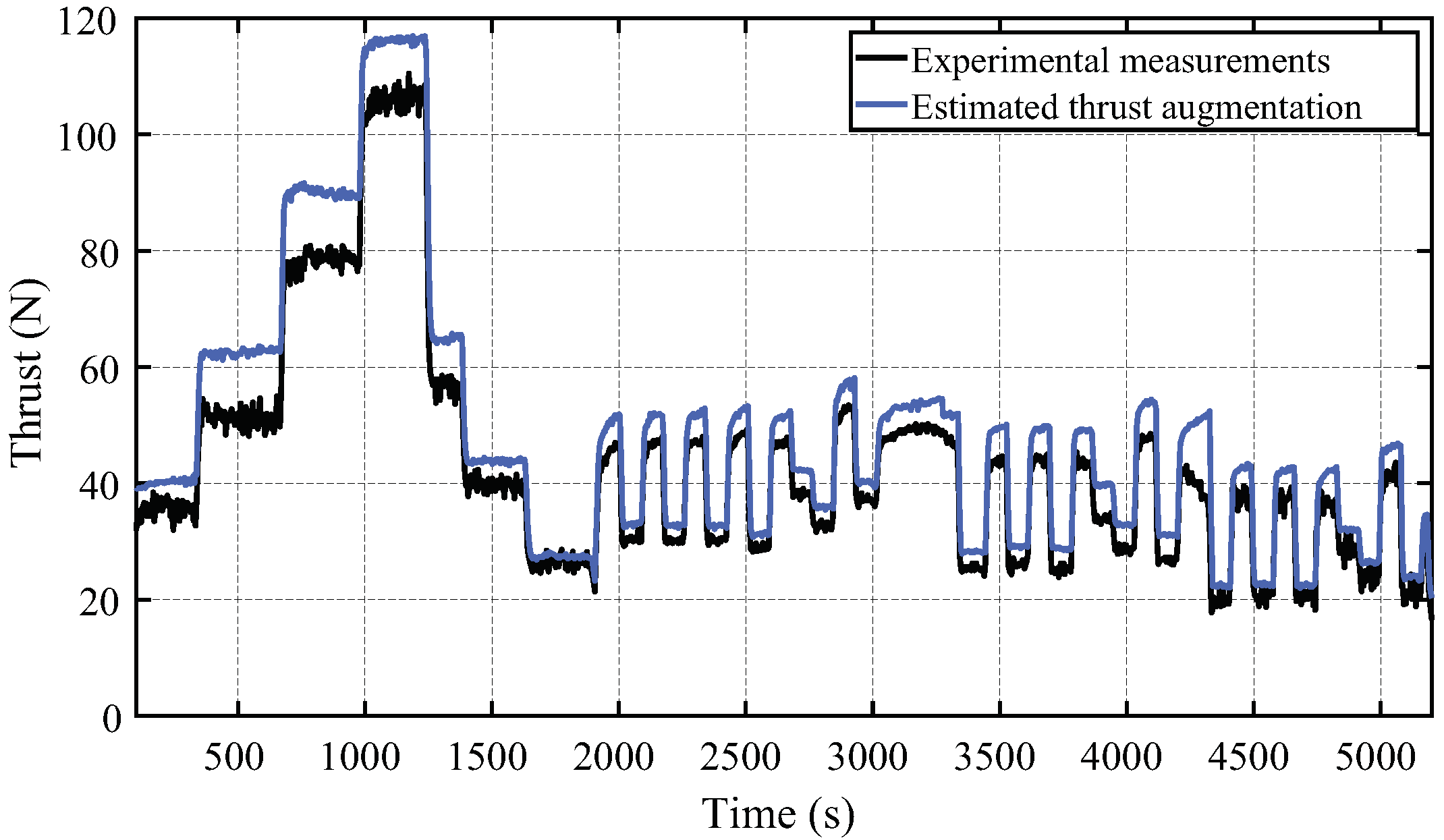
After optimally expanding the exhaust gas it is expected for the turbojet to provide an increased thrust with the same throttle settings. This result is confirmed in
Figure 20, which shows the estimated thrust with the proposed control scheme in comparison with the measurements using a fixed nozzle turbojet. The thrust is estimated to increase up to 20 %. For the whole experiment considering different maneuvers and throttle settings, the average percentile augmented thrust is 14.41%. This thrust augmentation can provide major improvements for the turbojet fuel economy.
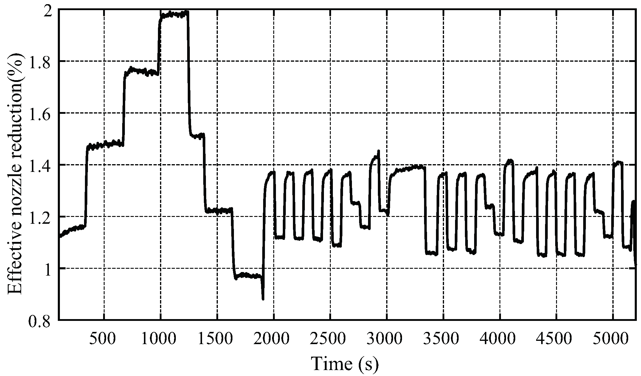
The effective nozzle area reduction is presented in
Figure 21. The nozzle adapts to the new throttle setting by increasing or reducing the output area according to the exhaust total pressure and ambient density, while rejecting the disturbances during transient operation. Since the nozzle is reduced most of the time to achieve optimal expansion, it is possible to conclude that the turbojet is probably designed to operate near sea-level conditions (larger ambient pressures) and it requires adaption to operate at higher altitudes.
6.2. Key Advantages of Variable Exhaust Nozzle Control
Firstly, it was demonstrated in
Section 3.2 that if only the disturbance rejection elements of the
LADRC are used, the resulting system retains the stability and performance properties of the plant controlled by the
LSC. This allowed designing the
LSC + LADRC considering the requirements stated from aeronautical certifications for high performance applications, shown in
Section 4.1. This simplifies the controller design process.
On the vein of fuel economy,
Figure 20 shows that the resulting thrust generated with a variable exhaust nozzle is greater in every condition tested at this particular application. This augmentation could allow reducing the operating thermal state (i.e., less fuel flow) to achieve the same mission when compared to a fixed exhaust nozzle. In consequence, variable exhaust nozzles can improve the fuel economy of aircraft propelled by small-scale turbojets.
Finally, a salient property can be observed when considering the stall margin, which is is one of the main serviceability limits of aeroengines [
32]. Although these margins are clearly defined for static operating conditions, when the aeroengine undergoes harsh maneuvers, the compressor faces a fast increase in the pressure ratio with a quasi-constant mass flow [
33]. Considering the causality of shaft speed, pressure and mass-flow, the following statement becomes clear: in the time period among the compressor pressure rise and the respective increase in the mass flow the static stall line limit can be exceeded, which may induce engine malfunction. To reduce this possibility, aeroengine controllers are designed to limit the thrust response velocity to avoid stall margin peaks and protecting the aeroengine structural safety. The implementation of a variable exhaust nozzle may allow operating the aeroengine more aggressively without reducing the stall margin (i.e., having a higher nozzle control bandwidth to increase the thrust without fuel flow modifications, as shown in
Figure 10 and
Figure 13). If the nozzle handles the fast dynamics of the thrust demand, then the fuel flow can be slowly adjusted to the new set-point without reducing the stall margin during fast transient conditions.
Thus, when considering practical applications, key properties of the resulting turbojet + variable exhaust nozzle control scheme are that it (i) is compatible with aeronautical controls certification metrics, (ii) reduces operating costs through fuel flow savings and (iii) opens the possibility of achieving a faster thrust response without sacrificing the engine serviceability limit margins.
7. Conclusions
A novel variable exhaust nozzle control scheme is presented in this article. The combination the closed-loop performance and classical control specifications of a loop-shaping-controller (LSC) with the disturbance rejection properties of a linear-active-disturbance-rejection controller (LADRC) is the major characteristic of this novel scheme. The LSC is designed to meet the robustness and performance requirements by needed in common aeronautical certifications, and to provide the desired closed-loop characteristics.
The proposed approach integrates the LADRC with a classical LSC in such a manner that the system robustness margins are completely defined by the LSC. This key finding allows designing the LSC and LADRC independently with well-known design tools. This is a powerful combination that maintains the properties of well-known classical linear controllers with a modern perspective on disturbance rejection.
On the other hand, a novel mathematical representation of the nozzle dynamics was obtained from first principles and adapted into the control-loop to achieve a stream-velocity-based control loop. The integration of this nozzle model allowed developing a clear approach to improve the exhaust gas expansion by increasing the exhaust gas speed up to the optimum expansion speed. This speed is defined by the turbojet exhaust gas total pressure and the ambient pressure. Due to the incompressibility assumption, the resulting algorithm is limited to operate under small exhaust gas speed changes. Salient properties of the proposed control scheme of the variable exhaust nozzle are that the resulting turbojet+variable exhaust nozzle control scheme:
Increases the produced thrust for the whole turbojet operating range by optimizing the flow expansion.
Highly reduces the input disturbance sensitivity when compared to classical controllers.
Maintains homogeneous performance properties along the operating range.
Is compatible with aeronautical control certifications.
Opens the possibility for achieving a faster thrust response without reducing the margin limits in transient operation.
Implementing the variable nozzle requires introducing hardware and software modifications to the turbojet; which in addition of increasing initial cost, can also result in additional weight. These modifications can include integrating additional sensors, actuators as well as the respective controller design. These are important considerations that must be weighted against possible benefits in any practical application. In this context, the results using real operational data from a turbojet showed that it is possible to increase the thrust production of the analyzed micro turbojet up to 20% when using an adaptive exhaust nozzle in combination with the proposed controller. The total augmented thrust adds up rapidly, requiring less fuel to operate within the same flight envelope and reducing the breach for a more environment-friendly operation. Finally, it can be concluded that applications that require multiple thrust set-points during operation could indeed benefit from this modification.
Author Contributions
Conceptualization, F.V.-V.; methodology, L.A.-B.; software, F.V.-V.; validation, D.H.-A.; formal analysis, F.V.-V. and L.A.-B.; investigation, P.Z.-R. and D.H.-A.; resources, P.Z.-R.; data curation, F.V.-V.; writing—original draft preparation, F.V.-V.; writing—review and editing, L.A.-B. and D.H.-A.; visualization, F.V.-V.; supervision, L.A.-B.; project administration, P.Z.-R.; funding acquisition, P.Z.-R. All authors have read and agreed to the published version of the manuscript.
Funding
This research was funded by CONACYT under the program Fondo Institucional de Fomento Regional para el Desarrollo Científico, Tecnológico y de Innovación FORDECYT. The APC was funded by Universidad de Monterrey and Universidad Autónoma de Nuevo León.
Institutional Review Board Statement
Not applicable.
Informed Consent Statement
Not applicable.
Data Availability Statement
Some or all data, models, or code that support the findings of this study are available from the corresponding author upon reasonable request.
Acknowledgments
The authors would like to thank the support provided by the “Fondo Institucional de Fomento Regional para el Desarrollo Científico, Tecnológico y de Innovación” from CONACYT (FORDECYT).
Conflicts of Interest
The authors declare no conflict of interest.
References
- Sundararaj, R.H.; Sekar, T.C.; Arora, R.; Kushari, A. Effect of nozzle exit area on the performance of a turbojet engine. Aerosp. Sci. Technol. 2021, 116, 106844. [Google Scholar] [CrossRef]
- Giorgio, Z.; Moggia, S.; Capobianco, M. Effects of a dual-loop exhaust gas recirculation system and variable nozzle turbine control on the operating parameters of an automotive diesel engine. Energies 2017, 1, 47. [Google Scholar]
- Szymon, F.; Chmielewski, M.; Gieras, M. Variable Geometry in Miniature Gas Turbine for Improved Performance and Reduced Environmental Impact. Energies 2020, 19, 5230. [Google Scholar]
- Villarreal-Valderrama, F.; Delgado, C.S.; Zambrano-Robledo, P.D.C.; Amezquita-Brooks, L. Turbojet direct-thrust control scheme for full-envelope fuel consumption minimization. Aircr. Eng. Aerosp. Technol. 2020, 93, 437–447. [Google Scholar] [CrossRef]
- Villarreal-Valderrama, F.; Liceaga-Castro, E.; Zambrano-Robledo, P.; Amezquita-Brooks, L. Experimental Evaluation of Different Microturbojet EGT Modeling Approaches. J. Aerosp. Eng. 2021, 34, 04020087. [Google Scholar] [CrossRef]
- Kisszölgyémi, I.; Beneda, K.; Faltin, Z. Linear quadratic integral (LQI) control for a small scale turbojet engine with variable exhaust nozzle. In Proceedings of the 2017 International Conference on Military Technologies (ICMT), Brno, Czech Republic, 31 May–2 June 2017; pp. 507–513. [Google Scholar]
- Andoga, R.; Főző, L.; Kovács, R.; Beneda, K.; Moravec, T.; Schreiner, M. Robust control of small turbojet engines. Machines 2019, 7, 3. [Google Scholar] [CrossRef] [Green Version]
- Tang, W.; Wang, L.; Gu, J.; Gu, Y. Single neural adaptive PID control for small UAV micro-turbojet engine. Sensors 2020, 20, 345. [Google Scholar] [CrossRef] [PubMed] [Green Version]
- Montazeri-Gh, M.; Rasti, A.; Jafari, A.; Ehteshami, M. Design and implementation of MPC for turbofan engine control system. Aerosp. Sci. Technol. 2019, 92, 99–113. [Google Scholar] [CrossRef]
- Surendran, S.; Chandrawanshi, R.; Kulkarni, S.; Bhartiya, S.; Nataraj, P.S.; Sampath, S. Model predictive control of a laboratory gas turbine. In Proceedings of the 2016 Indian Control Conference (ICC), Hyderabad, India, 4–6 January 2016; pp. 79–84. [Google Scholar]
- Shehata, A.M.; Khalil, M.K.; Ashry, M.M. Controller Design for Micro Turbojet Engine. In Proceedings of the 2020 12th International Conference on Electrical Engineering (ICEENG), Cairo, Egypt, 7–9 July 2020; pp. 436–440. [Google Scholar]
- Shi, G.; Wu, Z.; He, T.; Li, D.; Ding, Y.; Liu, S. Shaft speed control of the gas turbine based on active disturbance rejection control. IFAC-PapersOnLine 2020, 53, 12523–12529. [Google Scholar] [CrossRef]
- Juan, F.; Luo, M.; Wang, J.; Hu, Z. FMI-Based Multi-Domain Simulation for an Aero-Engine Control System. Aerospace 2021, 7, 180. [Google Scholar]
- Seonghee, K.; Park, H. Design of the Electronic Engine Control Unit Performance Test System of Aircraft. Aerospace 2021, 6, 158. [Google Scholar]
- Singh, R.; Maity, A.; Nataraj, P.S.V. Shaft Speed Control of Laboratory Gas Turbine Engine. IFAC-PapersOnLine 2019, 52, 262–267. [Google Scholar] [CrossRef]
- Giorgi, D.; Grazia, M.; Strafella, L.; Ficarella, A. Neural Nonlinear Autoregressive Model with Exogenous Input (NARX) for Turboshaft Aeroengine Fuel Control Unit Model. Aerospace 2021, 8, 206. [Google Scholar] [CrossRef]
- Farokhi, S. Aircraft Propulsion; John Wiley and Sons: Hoboken, NJ, USA, 2014. [Google Scholar]
- El-Sayed Ahmed, F. Aircraft Propulsion and Gas Turbine Engines; CRC Press: Boca Raton, FL, USA, 2017. [Google Scholar]
- Gang, T.; Gao, Z. Frequency response analysis of active disturbance rejection based control system. In Proceedings of the 2007 IEEE International Conference on Control Applications, Singapore, 1–3 October 2007; pp. 1595–1599. [Google Scholar]
- Gernot, H. A simulative study on active disturbance rejection control (ADRC) as a control tool for practitioners. Electronics 2013, 2, 246–279. [Google Scholar]
- Jin, H.; Liu, L.; Lan, W.; Zeng, J. On stability and robustness of linear active disturbance rejection control: A small gain theorem approach. In Proceedings of the 2017 36th Chinese Control Conference (CCC), Dalian, China, 26–28 July 2017; pp. 3242–3247. [Google Scholar]
- US Department of Transportation. CFR14 Part 33: Airworthiness Standards: Aircraft Engines; Federal Aviation Administration: Washington, DC, USA, 2015; pp. 1–300.
- Department of Defense. Flying Qualities of Piloted Aircraft; MIL-STD-1797A; Revision B; Military and Government Specs and Standards (Naval Publications and Form Center): Philadelphia, PA, USA, 2006; p. 235.
- Department of Defense. Airworthiness Certification Criteria; MIL-HDBK-516C; Revision A; Military and Government Specs and Standards (Naval Publications and Form Center): Philadelphia, PA, USA, 2014.
- Yazar, I.; Kiyak, E.; Caliskan, F.; Karakoc, T.H. Simulation-based dynamic model and speed controller design of a small-scale turbojet engine. Aircr. Eng. Aerosp. Technol. 2018, 90, 351–358. [Google Scholar] [CrossRef]
- Rakesh, B.; Maghade, P.D.K.; Sondkar, S.Y.; Pawar, S.N. A review of PID control, tuning methods and applications. Int. J. Dyn. Control 2020, 9, 818–827. [Google Scholar]
- Ahmad, S.; Keel, L.H. Robust lead-lag compensation for a family of uncertain linear systems. In Proceedings of the 1992 IEEE International Symposium on Circuits and Systems, San Diego, CA, USA, 10–13 May 1992; pp. 2716–2719. [Google Scholar]
- Villarreal-Valderrama, F.; Takano, L.; Liceaga-Castro, E.; Hernandez-Alcantara, D.; Zambrano-Robledo, P.; Amezquita-Brooks, L. An integral approach for aircraft pitch control and instrumentation in a wind-tunnel. Aircr. Eng. Aerosp. Technol. 2020, 92, 1111–1123. [Google Scholar] [CrossRef]
- Khustochka, O.; Yepifanov, S.; Zelenskyi, R.; Przysowa, R. Estimation of performance parameters of turbine engine components using experimental data in parametric uncertainty conditions. Aerospace 2020, 7, 6. [Google Scholar] [CrossRef] [Green Version]
- Slotine, J.-J.E.; Li, W. Applied Nonlinear Control; Prentice Hall: Englewood Cliffs, NJ, USA, 1991; Volume 1. [Google Scholar]
- Lin, F.T. Robust Control Design: An Optimal Control Approach; John Wiley Sons: Hoboken, NJ, USA, 2007; Volume 1. [Google Scholar]
- Dvirnyk, Y.; Pavlenko, D.; Przysowa, R. Determination of serviceability limits of a turboshaft engine by the criterion of blade natural frequency and stall margin. Aerospace 2019, 6, 132. [Google Scholar] [CrossRef] [Green Version]
- Jiři, P.; Jílek, A.; Kmoch, P. Small Jet Engine Centrifugal Compressor Stability Margin Assessment. In Turbo Expo: Power for Land, Sea and Air; American Society of Mechanical Engineers: New York, NY, USA, 2017; p. 50817. [Google Scholar]
Figure 1.
Diagram of variable exhaust nozzle geometrical characteristics.
Figure 1.
Diagram of variable exhaust nozzle geometrical characteristics.
Figure 2.
Surface plot of the possible values of the model parameter, , depending on the linearization point expressed in terms of and .
Figure 2.
Surface plot of the possible values of the model parameter, , depending on the linearization point expressed in terms of and .
Figure 3.
Nozzle control considering static pressure feedback.
Figure 3.
Nozzle control considering static pressure feedback.
Figure 4.
Wiener model structure of the output dynamic pressure. The linear element describes the exhaust gas velocity dynamics and the non-linear static gain transforms the exhaust gas velocity into its dynamic pressure equivalent.
Figure 4.
Wiener model structure of the output dynamic pressure. The linear element describes the exhaust gas velocity dynamics and the non-linear static gain transforms the exhaust gas velocity into its dynamic pressure equivalent.
Figure 5.
Controller structure considering the Wiener-model representation of the dynamic pressure. The nozzle constriction angle is the only mean for directly actuating over the flow speed in the nozzle while can be considered as input perturbations.
Figure 5.
Controller structure considering the Wiener-model representation of the dynamic pressure. The nozzle constriction angle is the only mean for directly actuating over the flow speed in the nozzle while can be considered as input perturbations.
Figure 6.
Simplification of the controller structure, segregating into the effects of the nozzle input (gas properties from the turbine output), and the nozzle output (gas expansion objectives).
Figure 6.
Simplification of the controller structure, segregating into the effects of the nozzle input (gas properties from the turbine output), and the nozzle output (gas expansion objectives).
Figure 7.
Linear Active Disturbance Rejection Control (LADRC) structure.
Figure 7.
Linear Active Disturbance Rejection Control (LADRC) structure.
Figure 8.
Combination of a Loop Shaping Control LSC with the disturbance rejection element of the LADRC.
Figure 8.
Combination of a Loop Shaping Control LSC with the disturbance rejection element of the LADRC.
Figure 9.
Equivalent representation of the LADRC + LSC, considering the transformation of the observer into a transfer function representation.
Figure 9.
Equivalent representation of the LADRC + LSC, considering the transformation of the observer into a transfer function representation.
Figure 10.
Unit step response with controllers of similar time-domain specifications.
Figure 10.
Unit step response with controllers of similar time-domain specifications.
Figure 11.
Disturbance rejection capabilities of the developed controllers.
Figure 11.
Disturbance rejection capabilities of the developed controllers.
Figure 12.
Unit step response with added band-limited white sensor noise of dBW.
Figure 12.
Unit step response with added band-limited white sensor noise of dBW.
Figure 13.
Open loop Bode plot of the developed controllers. Note that the LSC and the LADRC + LSC responses are identical, thus the LSC was not included.
Figure 13.
Open loop Bode plot of the developed controllers. Note that the LSC and the LADRC + LSC responses are identical, thus the LSC was not included.
Figure 14.
Comparison of the LSC and the LADRC + LSC schemes in terms of noise sensitivity, dashed lines, and input disturbance sensitivity, solid lines.
Figure 14.
Comparison of the LSC and the LADRC + LSC schemes in terms of noise sensitivity, dashed lines, and input disturbance sensitivity, solid lines.
Figure 15.
Upper and lower sectors containing the non-linear transformation.
Figure 15.
Upper and lower sectors containing the non-linear transformation.
Figure 16.
Autonomous representation of the pressure-control loop considering the exhaust gas speed non-linear static transformation with the model uncertainty limits and .
Figure 16.
Autonomous representation of the pressure-control loop considering the exhaust gas speed non-linear static transformation with the model uncertainty limits and .
Figure 17.
Asymptotic stability test for the nozzle control with the non-linear static gain and modeling uncertainty.
Figure 17.
Asymptotic stability test for the nozzle control with the non-linear static gain and modeling uncertainty.
Figure 18.
Reference tracking for the velocity to achieve optimal expansion of the exhaust gas.
Figure 18.
Reference tracking for the velocity to achieve optimal expansion of the exhaust gas.
Figure 19.
Disturbances caused by the turbojet change the operating thermal state, .
Figure 19.
Disturbances caused by the turbojet change the operating thermal state, .
Figure 20.
Estimations of the augmented thrust computed with the LADRC + LSC controlled nozzle exhaust gas speed.
Figure 20.
Estimations of the augmented thrust computed with the LADRC + LSC controlled nozzle exhaust gas speed.
Figure 21.
Effective nozzle area reduction when operating at different thermal states.
Figure 21.
Effective nozzle area reduction when operating at different thermal states.
Table 1.
Non-linear models performance metrics.
Table 1.
Non-linear models performance metrics.
| Indicator | PI | LSC | LADRC | LADRC + LSC |
|---|
| Gain margin (dB) | | | | |
| Phase margin (deg) | 103 | | | |
| Bandwidth (rad/s) | | | | |
| Publisher’s Note: MDPI stays neutral with regard to jurisdictional claims in published maps and institutional affiliations. |
© 2021 by the authors. Licensee MDPI, Basel, Switzerland. This article is an open access article distributed under the terms and conditions of the Creative Commons Attribution (CC BY) license (https://creativecommons.org/licenses/by/4.0/).


 ,
, 


