Article

Orbital Design and Control for Jupiter-Observation Spacecraft

1
State Key Laboratory of Astronautic Dynamics, Xi’an Satellite Control Center, Xi’an 710043, China
2
School of Electronic and Information Engineering, Xi’an Jiaotong University, Xi’an 710049, China
*
Author to whom correspondence should be addressed.
Aerospace 2021, 8(10), 282; https://doi.org/10.3390/aerospace8100282
Submission received: 28 July 2021 / Revised: 18 September 2021 / Accepted: 25 September 2021 / Published: 1 October 2021
(This article belongs to the Special Issue Spacecraft Dynamics and Control)

Abstract

:
This paper investigates the evolution of orbits around Jupiter and designs a sun-synchronous repeating ground track orbit. In the dynamical models, the leading terms of the Jupiter’s oblateness are J2 and J4 terms. A reasonable range of ground track repetition parameter Q is given and the best observation orbit elements are selected. Meanwhile, the disturbing function acting on the navigation spacecraft is the atmospheric drag and the third body. The law of altitude decay of the spacecraft’s semimajor orbit axis caused by the atmospheric drag is studied, and the inclination perturbation caused by the sun’s gravity is analyzed. This paper designs a semimajor axis compensation strategy to maintain the orbit’s repeatability and proposes an initial inclination prebiased strategy to limit the local time at the descending node in a permitted range. In particular, these two methods are combined in the context of sun-synchronous repeating ground track orbit for better observation of the surface of Jupiter.

1. Introduction

With advances in science and technology, people desire more to go into outer space for adventure, while an increasing number of scientists hope to explore other planets in the solar system. It is a long journey from the Earth to other planets. Many researchers have done a lot of work on trajectory optimization of deep space exploration. Most of these works are based on direct methods or indirect methods [1,2,3]. Not limited to impulse control situation, there are also several continuous thrust methods about interplanetary transfer. For instance, a design of low-thrust interplanetary trajectories with multiple gravity assists was described in [4]. An automated solution strategy for multiobjective optimal design of low-thrust multi-gravity-assist trajectories based on a two-step algorithm was proposed [5]. Some subjects were studied for academic use only, while some were mission-based [6,7,8]. Though there has been lots of work done on the deep space trajectory optimization, few studies have been carried out on the orbital control of spacecraft around the outer space planets [9,10,11,12]. Liu et al. [11] investigated quasicircular frozen orbits in the Martian gravity field and examined their basic nature analytically. In [12], authors proposed a continuous control method that combined analytical theory and parameter optimization to build an artificial frozen orbit of Mercury. Nevertheless, research on gaseous planets such as Jupiter is limited.
Jupiter, by far the largest planet in the solar system, was named after the king of the gods in Roman Mythology, Jupiter, the biggest and most powerful of all. It contains two thirds of the solar system mass outside the sun—twice the mass of all the other planets combined. Unlike the Earth, Mars and other major planets, Jupiter has no hard surface that we can see. Jupiter is a gas giant planet with a fascinating appearance. It has different colors from space observation which represent clouds with different compositions and different vertical structures [13]. The Jovian atmosphere shows a wide range of active phenomena, including band instabilities, vortices, storms, and lightning. The vortices reveal themselves as large red, white, or brown spots. In addition, Jupiter has the fastest rotation velocity of all planets in the solar system, leading to an unevenly distributed magnetic field [14]. The exploration of Jupiter could greatly enhance our understanding of the origin and evolution of the solar system.
Since the 1970s, several spacecraft have been launched aiming to flyby or enter the Jupiter system [15,16,17,18]. Project Galileo made a triumphant arrival at Jupiter on 7 December 1995. The Galileo Atmospheric Entry Probe became the first object to penetrate and directly measure the atmosphere of an outer planet [19]. In 2016, with the completion of measurement of gravitational field, magnetic field and magnetosphere of Jupiter, the Juno spacecraft gradually unveiled the mystery of Jupiter [20]. As a result, an increasing number of scholars have studied Jupiter’s space environment and its moons. Liu et al. [21] described the physical environment for the Jovian dust dynamics, including the gravity, the magnetic field, and the plasma environment. Liu et al. [22] studied the characteristics of four special types of Jovian orbits and offered analytical and numerical methods to achieve them. Most of these works focused on the natural environment, but few studies highlighted the control of spacecraft around the Jupiter.
The well-known spacecraft Juno ran in a highly elliptical orbit of Jupiter, and the spacecraft stayed near the apogee for a long time. This has a few advantages. First, it can be far away from Jupiter’s high radiation environment. Second, it can explore some Jovian satellites. However, the time for close observation of Jupiter is relatively limited. With continuous advances in technology in aerospace, spacecraft can undoubtedly get closer to the surface of Jupiter. The spacecraft are expected to observe the surface of Jupiter closely for a long time in a wide range of latitudes. The sun-synchronous repeating ground track orbit can well support such observations. China announced that it would tackle key technical problems in the exploration of Jupiter system in the next few years [23]. This huge mission includes not only the detection of the fantasy phenomena of Jovian surface but also of the space environment around Jupiter. The lighting angle between the sun-synchronous repeating ground track orbit and the sun is fixed and the repeatability of the orbit secures an unalterable solar local time. The consistent lighting conditions can satisfy the requirements of remote sensing and time resolution at the same time.
Several studies of the design of sun-synchronous orbit and the repeating ground track orbit have been done. Ortore et al. [24] designed periodic sun-synchronous orbits of both Mars and the Earth under the hypothesis of J2 predominant, but the gravitational field model used in the paper is too simple for Jupiter. Aorpimai et al. [25] designed a repeating ground track orbit for the Earth under the effect of drag. However, Jupiter rotates much faster than the Earth, which will make a big difference in the design of the repeating ground track orbit. Liu et al. [26] respectively analyzed the sun-synchronous and the repeating ground track orbit of Mars, but the sun-synchronous repeating ground track orbit was not examined in the paper. Some researchers also studied the orbit control. To be specific, a station keeping strategy for satellite formation was put forward in [27] under the effects of atmosphere drag. Similarly, a control for local solar time drift caused by the action of solar gravitational perturbations of sun-synchronous orbits was proposed in [28]. The models in the two studies leave much to be desired for Jupiter. A low-thrust control was executed in the artificial Martian sun-synchronous orbits [29], however, Jupiter is so far away from the Earth. In such case, impulse control is undoubtedly more suitable for Jupiter.
In this paper, we intend to design a sun-synchronous repeating ground track orbit to detect the wonderful landscape in a stable and long-term way. First, we offer a reasonable range of the most important parameter for sun-synchronous repeating ground track orbits and give the exact elements of the designed orbit. Then, the law of influence of the atmosphere on the spacecraft is analyzed and a solution to the decay of spacecraft’s orbital semimajor axis is provided. In addition, an initial inclination prebiased method is proposed to offset the influence on inclination caused by the sun’s gravity and limit the local time at the descending node in a permitted range. At last, a control strategy that considers the two above-mentioned perturbations is put forward to observe the surface of Jupiter in a stable and long-term way.

2. Orbit Selection for Jupiter-Observation

2.1. Sun-Synchronous Orbits

Sun-synchronous orbits are orbits with a precession rate of the orbital plane equal to the planetary revolution around the sun. As a result, it is conducive to the spacecraft’s temperature control and the design of the power supply system, and it is also conducive to the spacecraft‘s visible light remote sensing observations on the ground [30,31].
Due to the influence of the harmonic term of Jupiter’s gravitational field, the right ascension of the ascending node Ω of the spacecraft’s orbit will produce secular perturbations. Thanks to the Juno gravity measurement experiment [32], Jupiter’s gravity harmonics coefficients are obtained, from which one can see the Jupiter’s gravity field is dominated by J2 and J4.
Some terms of Jupiter’s gravity harmonics coefficients, such as, J 2 = 14,696.572 × 10 6 , J 3 = 0.042 × 10 6 , J 4 = 586.609 × 10 6 , J 5 = 0.069 × 10 6 , J 6 = 34.198 × 10 6 are measured in [32].
Considering the influence of the main terms J2 and J4, the right ascension of the ascending node precession rate arising from the secular perturbations of the first order [33] is
Ω ˙ 1 = 3 2 n J 2 R J 2 p 2 cos i
where n is the mean angular velocity of the spacecraft, RJ is the reference radius of the Jupiter, p = a 1 e 2 , a is the semimajor axis of the spacecraft’s orbit, e is the eccentricity of the orbit and i is the spacecraft’s orbital inclination.
The nodal precession rate arising from the secular perturbations of the second order [34] is
Ω ˙ 2 = 3 J 2 R J 2 p 2 2 n cos i 1 6 e 2 1 + 5 4 sin 2 i + 1 e 2 1 3 2 sin 2 i + 3 2 5 3 sin 2 i 35 8 J 4 R J 4 p 4 n cos i e 2 9 7 9 4 sin 2 i + 6 7 3 2 sin 2 i .
Therefore, the mean node precession rate is
Ω ˙ = Ω ˙ 1 + Ω ˙ 2 .
For sun-synchronous orbits, the rate of node precession is equal to the Jupiter mean motion around the sun. That is
Ω ˙ = n s
where ns is Jupiter’s mean motion around the sun.
Equation (4) can be further rearranged as
f cos i = α cos 3 i + β cos i + γ = 0
where α = 9 n J 2 2 R J 4 4 p 4 e 2 5 24 105 J 4 24 J 2 2 + 3 2 1 e 2 + 5 3 35 J 4 12 J 2 2 ; β = 3 n J 2 R J 2 2 p 2 1 + 3 J 2 R J 2 2 p 2 e 2 3 8 + 15 J 4 8 J 2 2 1 2 1 e 2 1 6 5 J 4 4 J 2 2 ;   γ = n s .
As we note that f cos i is the cubic function of cos i , Equation (5) probably has one, two, or three distinct roots in the interval. It is necessary to judge whether all roots of Equation (5) are meaningful for different semimajor axes. Based on the theory of the cubic equation, Equation (5) has three real roots if the discriminant satisfies the condition
Δ = γ 2 4 α 2 + β 2 27 α 3 0 .
Equation (5) has one real root and two complex roots if the discriminant satisfies the condition: Δ > 0 . Additionally, it is also necessary to avoid impact with the surface of Jupiter. Therefore, the semimajor axis a and eccentricity e should satisfy
R J < a 1 e .
Figure 1a illustrates the relation between a, e and the discriminant. Here we set semimajor axis a to change from RJ to 2RJ and e from 0 to 1 − RJ/a. From Figure 1a, one can see that the discriminant is always above zero, so Equation (5) has one real root all the time. In other words, it is evident that there usually only exists one sun-synchronous orbit at a certain semimajor axis with normal eccentricity. Figure 1b shows the variations of inclination i with respect to a and e. As one can see from Figure 1b that the inclination is always greater than 90 degrees, the sun-synchronous orbits of Jupiter must be retro-orbits.

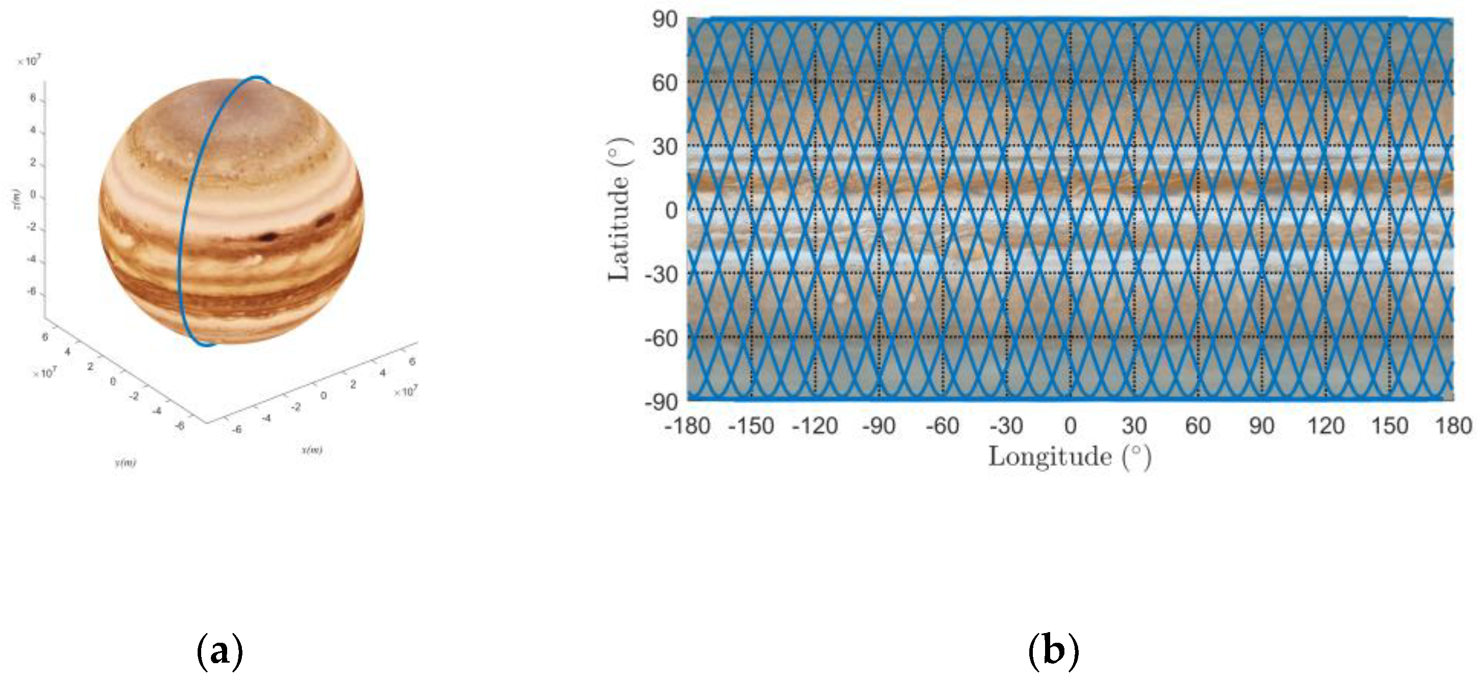
2.2. Repeating Ground Track Orbits

An important study in the design of spacecraft’s orbit for remote sensing is the global coverage problem. From application point of view, the composite of the area swept by the spacecraft remote sensing instrument over the ground should cover the entire surface of Jupiter, and it is then also required that the spacecraft traces the same track on the ground with a given periodicity pattern. The interval of the adjacent ground track in the equator is a combination of Jupiter’s rotation, orbital node precession, and spacecraft’s motion, which can be expressed as
Δ λ = T N ω Ω ,
where T N is the nodal period of the motion of the spacecraft, ω Ω is the Jupiter rotational angular speed relative to the ground track. It can be further obtained as
ω Ω = ω J Ω ¯ ˙ ,
where ω J is the rotational angular speed of Jupiter and Ω ¯ ˙ is the mean nodal precession rate. We use Ω ¯ ˙ = Ω ˙ in Equation (3).
To realize global coverage, the ground track should be periodic visited. The condition for repeating ground track orbits can be written as
R T N ω J Ω ¯ ˙ = R · Δ λ = N · 2 π
R T N = N D N
where R and N are both positive integers, D N = 2 π ω J Ω ¯ ˙ , which means the period Jupiter rotates relative to the spacecraft’s orbit. Equation (11) means the spacecraft runs R circles in N Jupiter nodal days.
The nodal period of the motion of the spacecraft T N can be expressed as
T N = 2 π M ˙ + ω ˙
where ω ˙ = ω ˙ 1 + ω ˙ 2 , which contains two parts: the secular perturbations of the first and the second order
ω ˙ 1 = 3 n J 2 R J 2 2 p 2 5 2 sin 2 i 2 ;
ω ˙ 2 = 9 n J 2 2 R J 4 p 4 e 2 7 12 3 8 sin 2 i 15 32 sin 4 i + 1 e 2 2 11 2 sin 2 i + 15 4 sin 4 i + 4 103 12 sin 2 i + 215 48 sin 4 i 35 J 4 18 J 2 2 e 2 27 14 27 4 sin 2 i + 81 16 sin 4 i + 12 7 93 14 sin 2 i + 21 4 sin 4 i .
Similarly, M ˙ = n + M ˙ 1 + M ˙ 2 [34].
M ˙ 1 = 3 n J 2 R J 2 2 p 2 1 3 2 sin 2 i 1 e 2 ;
M ˙ 2 = 9 n J 2 2 R J 4 4 p 4 1 e 2 1 2 1 3 2 sin 2 i 2 1 e 2 + e 2 10 3 26 3 sin 2 i + 103 12 sin 4 i + 5 2 19 3 sin 2 i + 233 48 sin 4 i + e 4 1 e 2 35 12 35 4 sin 2 i + 315 32 sin 4 i 35 J 4 18 J 2 2 e 2 9 14 45 14 sin 2 i + 45 16 sin 4 i .
Define
Q = R N = 2 π Δ λ = 1 ± C N .
In Equation (17), Q is called ground track repetition parameter, which is often used to describe repeating ground track orbits.
From Equations (9)–(12), one can get
Q = R N = M ˙ + ω ˙ ω J Ω ˙ .
If Q is set a value, a, e and i will be related by Equation (18).

2.3. Sun-Synchronous Repeating Ground Track Orbits

If the spacecraft is designed for observing specific regions on Jupiter, as opposed to global observations, sun synchronicity is not enough. Thus, if an orbit is a sun-synchronous orbit and it is also a repeating ground track orbit, it can be called a sun-synchronous repeating ground track orbit. It should satisfy Equations (4) and (18) at the same time. One can see both the expression of M ˙ and ω ˙ are quadratic function of sin 2 i from Equation (13) to Equation (16). Equation (18) can be further written as
M ˙ + ω ˙ = Q ω J n s
where ω J and n s are both constants for Jupiter. Thus, if the ground track repetition parameter Q is set a value, Equation (19) is a quadratic equation of variable about sin 2 i . Equation (19) can be rearranged as
Γ 1 sin 4 i + Γ 2 sin 2 i + Γ 3 Q ω J n s = 0
There exist meaningful roots only if the discriminant is greater than zero. That is
Δ = Γ 2 2 4 Γ 1 Γ 3 Q ω J n s 0
As the rotation angle velocity of Jupiter is greater than the Jupiter motion around the sun, the term ω J n s is greater than zero. As a result, Q has a minimum value
Q Γ 3 Γ 2 2 4 Γ 1 ω J n s
Due to the fact that the atmospheric drag dominates the perturbance forces at a too low height while observation is not convenient to conduct at a too high height, we select the orbit height about 2000 km above the Jupiter’s surface for a rough calculation of the value of Q. For h = 2000 km, the minimum value of Q can be calculated by the Equation (22), and the calculation result is about 2.97. Additionally, since the Jupiter rotates on its axis once every 9 h 55 min 30 s which is expressed as TJ. The orbit period of low-orbit spacecraft of Jupiter Tl is about 2 h 58 min 36 s. If we want a repeating ground track orbit to be meaningful, the maximum Q can be calculated based on T J / T l , and the outcome is approximately 3.33. As a conclusion, the meaningful ground track repetition parameter Q of Jupiter sun-synchronous repeating ground track orbit lies in (2.97, 3, 33).
It can be observed that Q lies in a quite narrow range. And it is important to decide the range for designing the sun-synchronous repeating ground track orbits.
Selecting the eccentricity e = 0.001, the relationship of inclination and semimajor axis for different Q is shown in Figure 2a. It can be seen that Q = 3.0, 3.1, 3.2 are sensible. Moreover, when Q increases to 3.3 the corresponding inclination will be less than 90 degrees which cannot satisfy the condition of sun-synchronous. Meanwhile, the discriminant will be less than zero if Q decreases to 2.9. When we draw the sun-synchronous a-i curve, it will intersect these three curves in Figure 2a. The intersections respectively correspond to three meaningful sun-synchronous repeating ground track orbits. The elements of the orbits are a = 1.06277 RJ, e = 0.001, i = 90.0996 deg with Q = 3.0; a = 1.03924 RJ, e = 0.001, i = 90.0925 deg with Q = 3.1 and a = 1.01692 RJ, e = 0.001, i = 90.0860 deg with Q = 3.2. For Q = 3.2 the orbit height of the spacecraft to Jupiter’s surface is about 1200 km, where the effect of atmospheric drag is so significant and the corresponding descending velocity of semimajor axis is 0.0054 m/s which means 467 m/day. The spacecraft’s orbit height will drop too fast. Obviously, it is an impractical maneuver. The detail of calculation is described in next chapter. For Q = 3.0 the height of spacecraft is about 4500 km, which is too high for observation. Only for Q = 3.1, the height of spacecraft is about 2800 km, which is suitable for long-term observation. Figure 2b shows the intersections of sun-synchronous orbit and repeating ground track orbit of Jupiter for Q = 3.1.
Liu et al. [24] once calculated the sun-synchronous repeating ground track orbit in his work, but he did not explicitly give the feasible range of Q. Meanwhile, the inclination of sun-synchronous repeating ground track orbit should not be less than 90 degrees which is not considered in his study. Most studies on the sun-synchronous repeating ground track orbit of the Earth lack the analysis of the feasible range of Q. The Earth rotates on its axis once every 24 h and the orbit period of low-orbit spacecraft of the Earth is about 90 min, therefore the maximum Q for the Earth is about 16, and there is a large range to select a feasible Q. It can be seen in the current research that a feasible Q rather than a range is given. Additionally, the methodology in this study can be generally applied to both Jupiter and other planets, though their dynamic models may differ. An analytic method is proposed to design the sun-synchronous repeating ground track orbit.
Figure 3a represents the sun-synchronous repeating ground track orbit of Jupiter during one period in a 3D view. The elements of the spacecraft’s orbit are a = 1.03924 RJ, e = 0.001, i = 90.0925 deg, Ω = 30 deg, w = 0 deg. The repeating parameter Q = 3.1 means that the spacecraft rotates around the Jupiter’s surface 31 revs in 10 Jupiter days. Figure 3b shows that during 10 Jupiter days, the ground tracks just close up with the starting point.

3. Perturbation and Control of Orbits around Jupiter

Since the spacecraft around Jupiter is perturbed by different kinds of forces, the orbit will change its trajectory and lose its sun synchronicity and repeatability. In that respect, atmospheric drag and the sun as third body are considered. The objective now is to derive a series of equations that allow to compute the maneuver frequency, size of the maneuver and impulse per maneuver that a spacecraft requires in order to maintain the spacecraft’s orbit in a ground track boundary which is defined by its mission requirements. In order to compute the maneuver frequency, it is first required to know the rate of change that the deviation of the ground track experiences over time. Once this result is obtained, the evolution of the ground track drift will be computed by the integration of its rate of change.

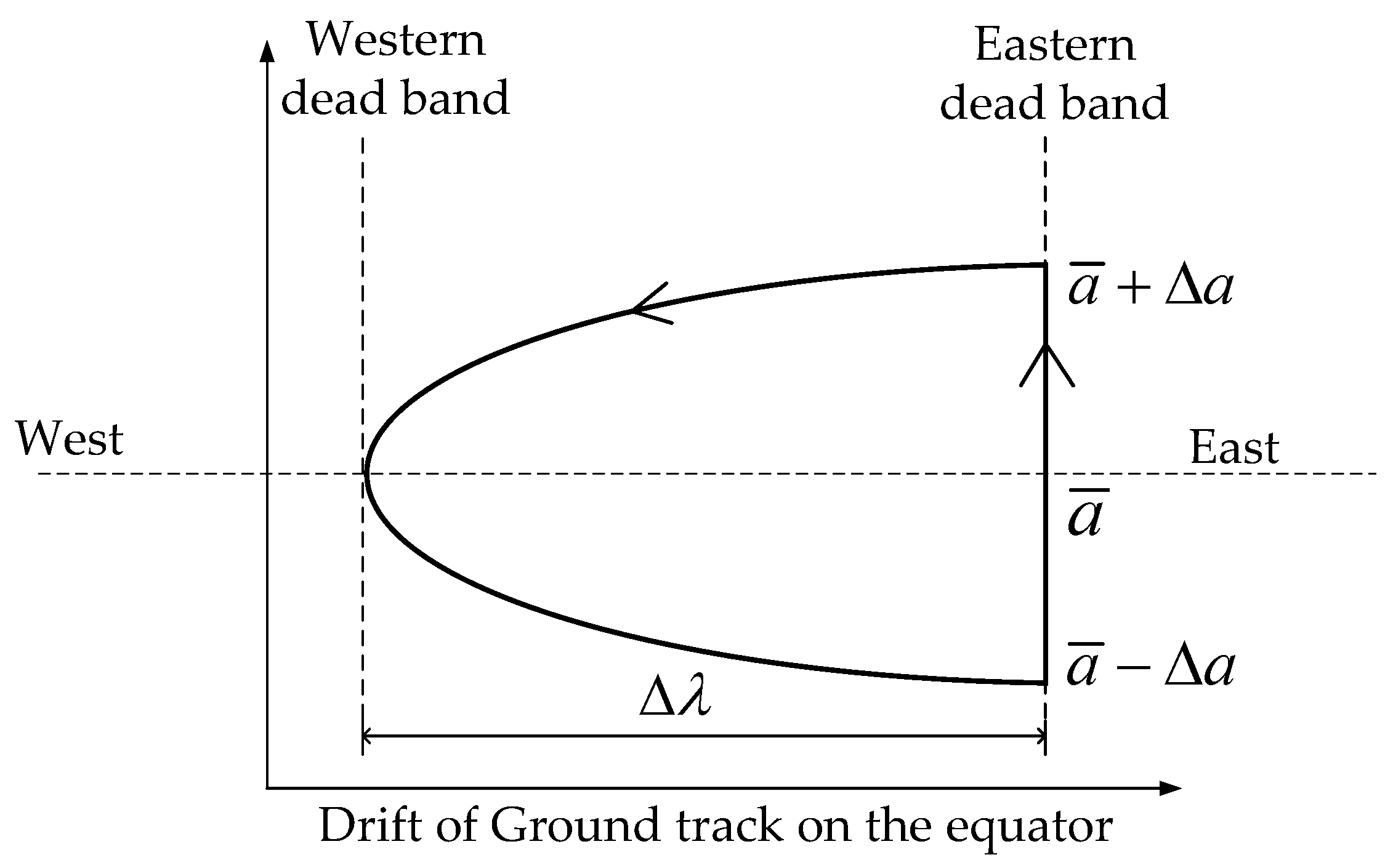
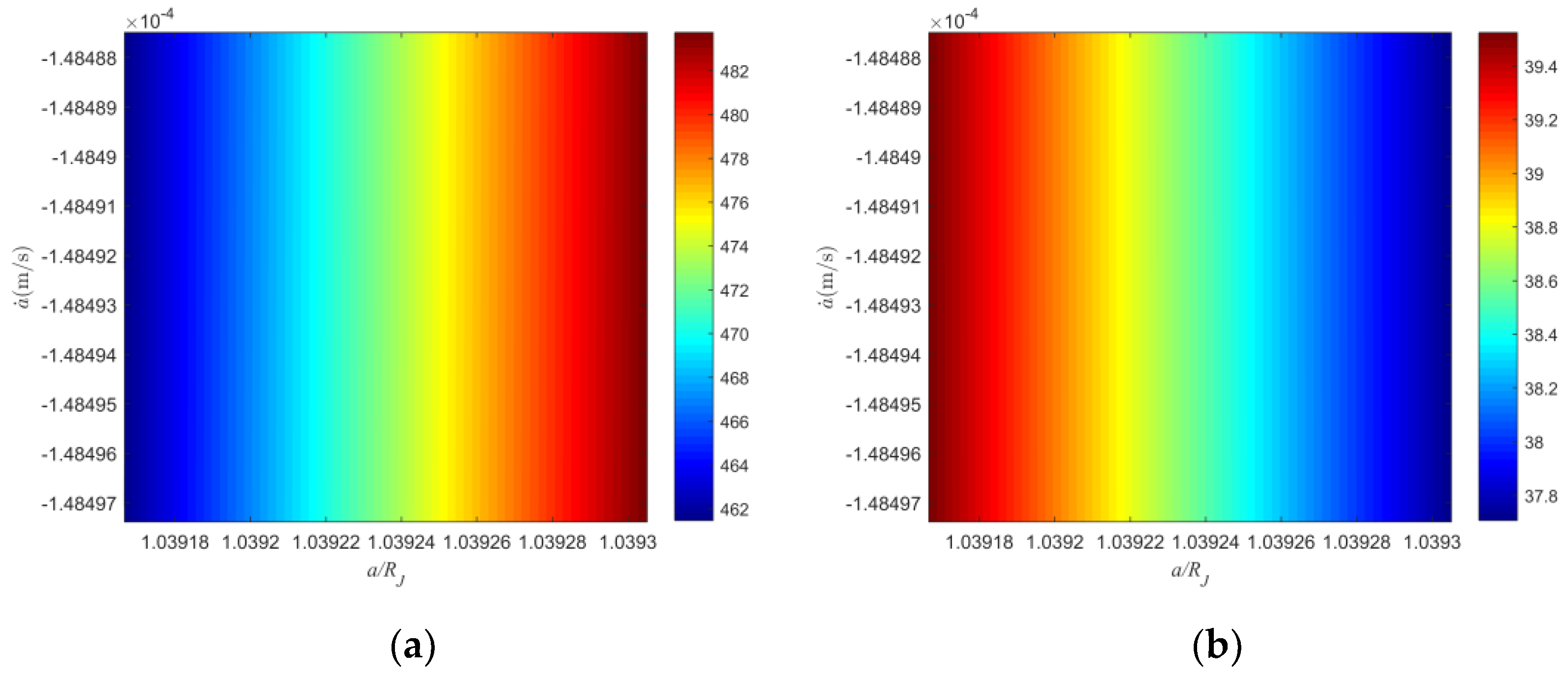
3.1. Influence on Semimajor Axis Caused by the Atmosphere

As Jupiter is composed of gases, the observation of Jupiter must consider the influence of the atmosphere on the spacecraft. Due to the influence of atmospheric drag, the semimajor axis of the orbit will be decayed. The lower the orbital height, the more obvious the decay. The resulting shortening of the orbital period causes the position of the ground track to drift eastward, which destroys the repeatability of the trajectory. As a result, it is necessary to execute periodic trajectory maintenance. The trajectory maintenance is achieved by periodic compensation for the decay of the semimajor axis. For spacecraft that do not require high stability or have a short operating life, only periodic compensation is enough to maintain the repeatability characteristics of the trajectory.
For the case of near circular orbits, the derivative of the semimajor axis can be approximated by
a ˙ = C d S ρ n a 2 m
where ρ is the atmospheric density in the spacecraft’s position, S is the cross-section area, m is the mass of the spacecraft, and Cd is the drag coefficient of the spacecraft.
For the convenience of calculation, the atmospheric density can be seen as a constant value for a given height. As a result, the change rate of semimajor axis caused by atmospheric can also be considered as a constant value.
The decay of the semimajor axis will cause the shortening of the orbital period, and the average angular velocity of the spacecraft will increase accordingly
δ n = 3 n ¯ 2 a ¯ δ a
δ a = a a ¯ , a = a 0 + a ˙ t
where a ¯ , n ¯ are nominal values, a is the semimajor axis which varies with time, a0 is the semimajor axis when t = 0. Therefore, the difference between the angular position of the spacecraft relative to the nominal position is
δ u = 0 t δ n d t = 3 n ¯ 2 a ¯ Δ a t + 1 2 a ˙ t 2
where Δ a = a 0 a ¯ .
Let λ be the angle shifted with respect to the nominal definition that the ground track has experienced over the equator at a given period t. The maintenance of orbits is essentially to control the drift λ of the spacecraft relative to the standard trajectory on the equator, and to limit λ within a permitted range during the entire spacecraft mission period. The difference of longitude between the real orbit and nominal orbit can be obtained as
δ λ = ω J n ¯ δ u = 3 ω J 2 a ¯ Δ a t + 1 2 a ˙ t 2
where ω J is the angular velocity of Jupiter as defined in Equation (9). Let ω J = 2 π D , where D is the Jupiter day. Equation (27) can be obtained
δ λ = 3 π a ¯ Δ a t + 1 2 a ˙ t 2
In Equation (28) the unit of t is rad/D, rather than rad/s. It can be seen that Equation (28) is a quadratic equation about time variable t. As it is known that a ˙ < 0 , a conclusion is that if a 0 a ¯ , δ λ will monotonically increase with time from Equation (28). As a result, the ground track drifts towards the east. However, if we execute a control maneuver to make Δ a > 0 at this moment, the ground track will drift towards the west. From Equation (28), the derivative of δ λ is
d δ λ d t = 3 π a ¯ Δ a + a ˙ t .
Let t s = Δ a a ˙ . When t = t s , we get
a = a ¯ , d δ λ d t = 0 , δ λ = 3 π Δ a 2 2 a ¯ a ˙ .
The ground track stops drifting westward but eastward instead. When t = 2 t s , we get
a = a ¯ Δ a , δ λ = 0 , d δ λ d t = 3 π Δ a a ¯ > 0 .
At this moment, the ground track drifts to the position at t = 0 . If we execute a maneuver on the semimajor axis to make it promote to the value at t = 0 .
a = a 0 = a ¯ + Δ a
the ground track will drift back towards the west again and repeat the process.
Figure 4 shows the relationship of the changing semimajor axis and the drift of ground track. Let
Δ λ = 3 π Δ a 2 2 a a ¯
be the total dead band size as Figure 4 has shown. The variation that the semimajor axis experiences can be obtained:
Δ a = 2 a ¯ a ˙ Δ λ 3 π .
Under the above control maneuver, the practical trajectory keeps between the western and eastern dead band in Δ λ 2 . When the trajectory moves to the eastern dead band, a control impulse will be added, whose size is Δ a and the time frequency between each maneuver is 2 Δ a a ˙ .
We limit the ground track drift to the nominal definition less than 50 km over the Jupiter equator. This means that the angle drift is about 0.04 deg, which is really a small and permissible angle error for Jupiter spacecraft observation. We assume that the spacecraft’s area-mass ratio S/m in Equation (23) is 0.02 m2/kg, and drag coefficient Cd is 2.2. As it has been calculated in the previous chapter, the semimajor axis is 1.03924 RJ, in other words, about 2805 km above Jupiter’s surface. Considering the initial error of semimajor axis when the spacecraft enters the Jupiter’s surrounding orbit, we select the spacecraft’s height from 2800 km to 2810 km above Jupiter’s surface. As we do not know the exact relationship between the atmospheric density and the spacecraft’s height, we just give the corresponding density range as described in [35,36]. Figure 5a illustrates that the control impulse varies with semimajor axis and the derivative of the semimajor axis. The corresponding a ˙ is calculated using Equation (23). Figure 5b shows the control frequency varies with a and a ˙ . From Figure 5a,b, an immediate conclusion can be obtained that the semimajor axis should be compensated about 462 to 482 m every 37.8 to 39.4 days under the effect of the atmospheric drag to keep the orbit’s repeatability. It can be found in Figure 5a that the compensation of semimajor axis increases with a on the x-axis. According to Figure 5b, the control frequency obtains the opposite results. On the y-axis, the compensation does not change obviously. These indicate that the effect of a changing semimajor axis dominates the result with respect to the changing density.

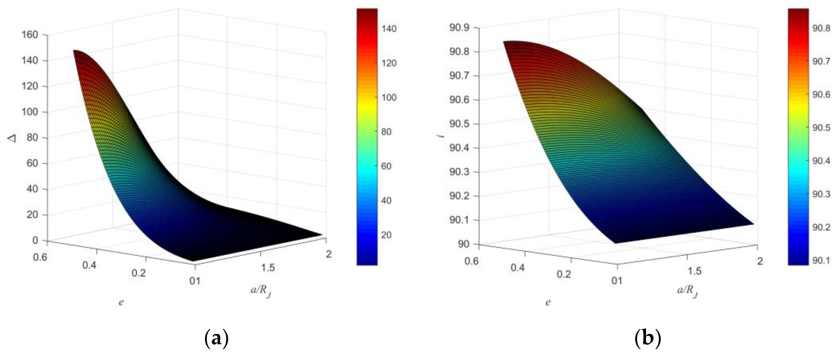
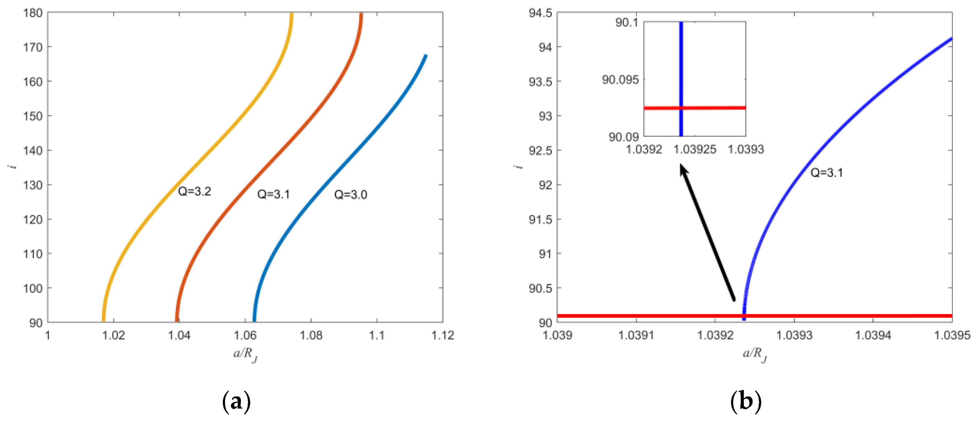
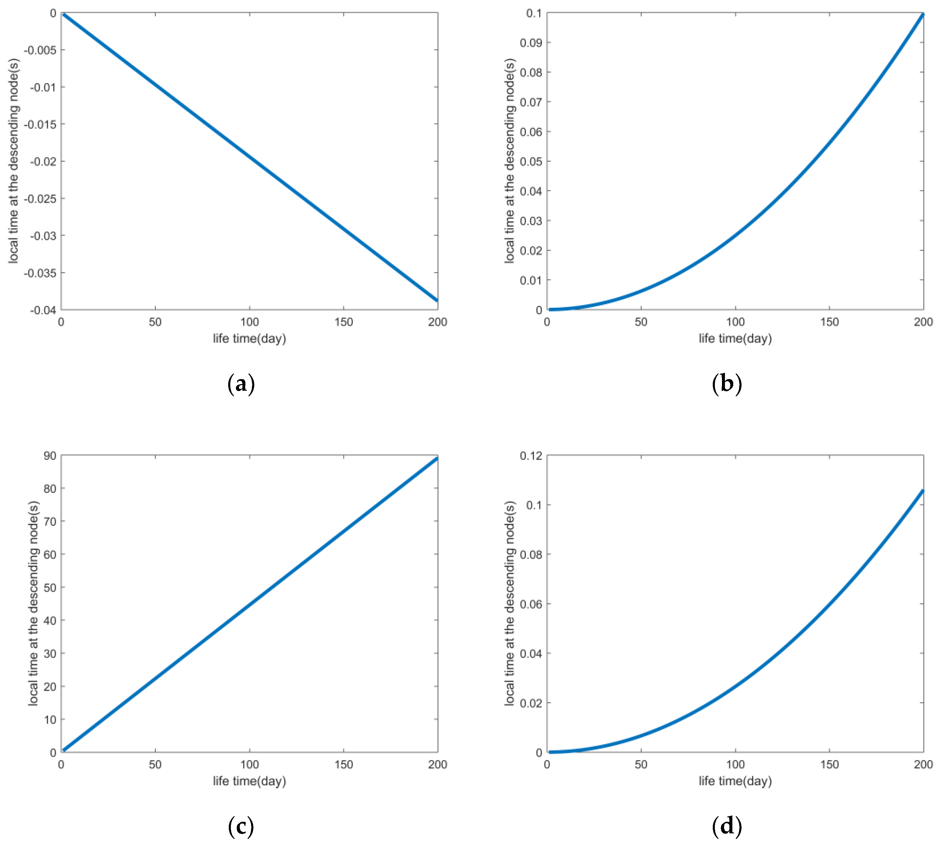
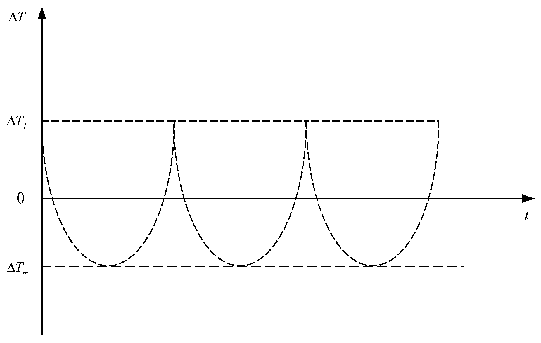
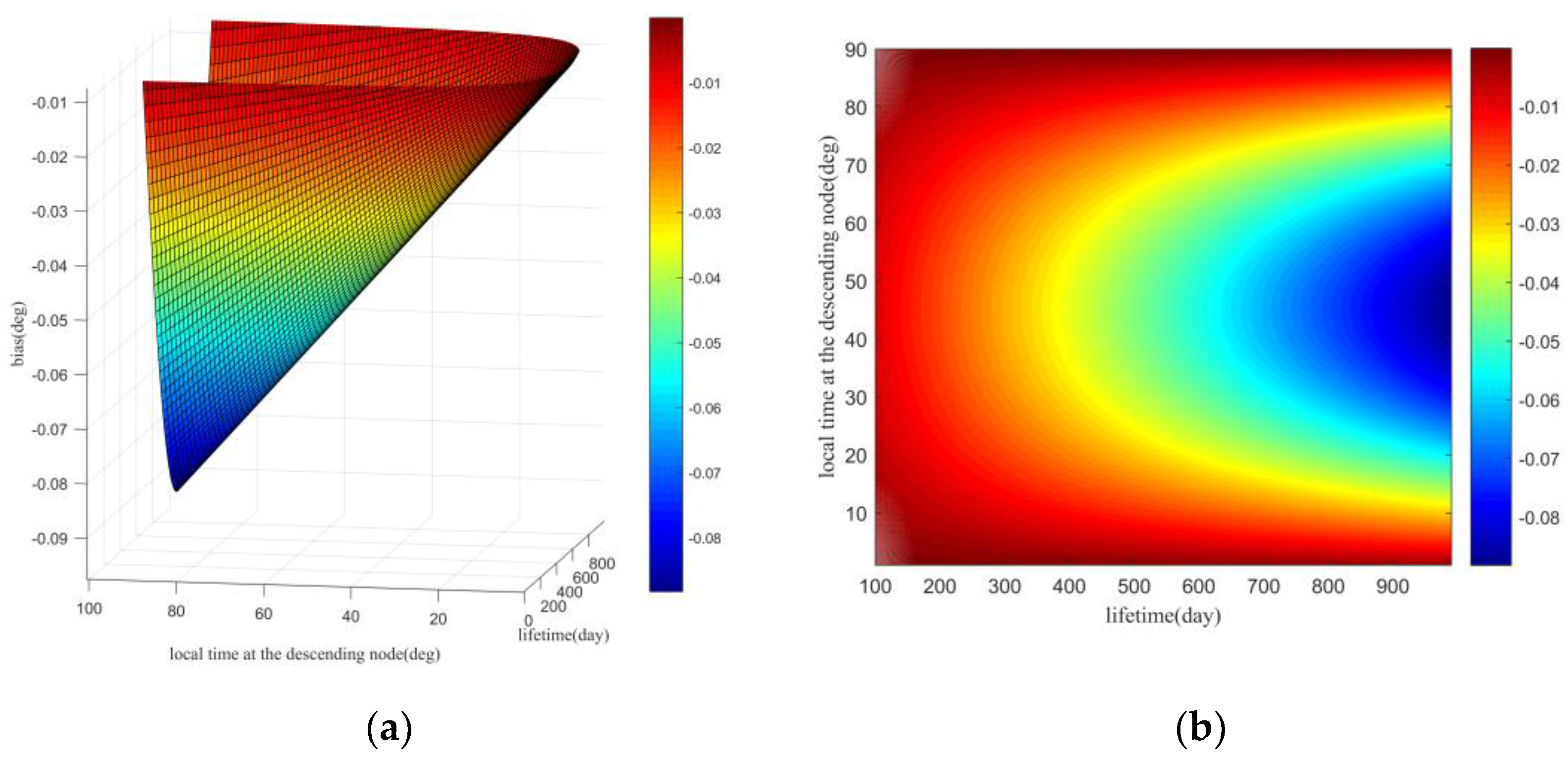
3.2. Influence on Orbital Inclination Caused by the Sun’s Gravity

The Jupiter spacecraft is always at the side of the sun, so the perturbation of the orbital inclination caused by the sun’s gravity must be considered. An additional control impulse should be executed to compensate the orbital inclination error. The change of orbital inclination caused by the sun’s gravity will bring two main effects. One is the change of local time at descending node; the other is the change of nominal orbit semimajor axis. In this paper, only the change of local time at the descending node is considered. In this chapter, an inclination prebiased compensatory strategy is proposed.
The derivative of inclination caused by the sun’s gravity can be obtained as [37]
i ˙ = cos ω + f n a F 0 = 3 r n s 2 cos ω + f cos ξ n a cos β s sin i sin Ω sin β s cos i s sin i cos Ω + sin β s sin i s cos i ,
where F 0 is the perturbation force caused by sun’s gravity along normal, β s is ecliptic longitude of apparent motions of the sun, i s is the angle between Jupiter’s motion around the sun and Jupiter’s equator, f is the true anomaly, ξ is the angle between two vectors. One is from the center of Jupiter to the spacecraft, and the other is from the center of Jupiter to the sun.
Given that the secular perturbations of cos ω + f cos ξ is
1 2 cos β s cos Ω + 1 2 sin β s cos i s sin Ω
the secular perturbations of the product of the above formula and cos β s sin i sin Ω sin β s cos i s sin i cos Ω + sin β s sin i s cos i is
1 4 sin i sin Ω cos Ω 1 4 cos i s 2 sin i sin Ω cos Ω + 1 4 sin i s cos i s sin Ω cos i .
Therefore, the secular rate of change of the spacecraft’s orbital inclination caused by the sun’s gravity perturbation is
i ˙ = 3 n s 2 2 n cos β s cos Ω + sin β s cos i s sin Ω · cos β s sin i sin Ω sin β s cos i s sin i cos Ω + sin β s sin i s cos i ,
where n s is Jupiter’s mean motion around the sun. If we ignore the influence of the period term of β s , the above formula can be rewritten as
i ˙ = 3 n s 2 8 n sin 2 Ω sin i + sin 2 i s sin Ω cos i sin 2 Ω cos 2 i s sin i = 3 n s 2 8 n sin i sin 2 Ω sin 2 i s + cos i sin Ω sin 2 i s .
If the orbit is sun-synchronous, β ˙ s = Ω ˙ is obtained. As a result, the term β s Ω corresponds to a constant. Equation (39) can be rewritten as a simple form:
i ˙ = 3 n s 2 16 n sin i 1 + cos i s 2 sin 2 β s 2 Ω
where β s Ω is corresponding to the local time at the descending node. From Equation (40), a conclusion can be obtained as: if the local time at the descending node is selected, the derivation of orbital inclination is constant. The derivation of Ω ˙ can be approximated with first-order Taylor expansion as
Δ Ω ˙ = Ω ˙ i Δ i + Ω ˙ a Δ a
where Δ i , Δ a are bias of i, a. Δ i , Δ a can be linearized as
Δ i = Δ i 0 + i ˙ t , Δ a = Δ a 0 + a ˙ t ,
where t is the on-orbit operation time of spacecraft. The bias in the formula above includes the initial launch error Δ i 0 , Δ a 0 and the perturbation i ˙ , a ˙ during the orbital period. As a result, Equation (41) can be further rearranged as
Δ Ω ˙ = Ω ˙ i Δ i 0 + Ω ˙ a Δ a 0 + Ω ˙ i i ˙ + Ω ˙ a a ˙ t
where i ˙ and a ˙ are defined in Equations (40) and (23). After a series of calculation, we find that only secular perturbations of the first order of node are enough for the analysis of drifting of local time. As a result, Equation (41) can be further written as
Δ Ω ˙ = 7 Ω ˙ 2 a Δ a Ω ˙ tan i Δ i
Through integrating Δ Ω ˙ in Equation (44), Δ Ω can be obtained using the following expression
Δ Ω t = Δ Ω t 0 7 Ω ˙ 2 a Δ a t 0 t t 0 7 Ω ˙ 4 a a ˙ t t 0 2 Ω ˙ tan i Δ i t t 0 1 2 Ω ˙ tan i i ˙ t t 0 2 .
We change the unit from rad and second to degree and day. As Ω ˙ changes 360 degrees in a Jupiter year, it means Ω ˙ = 0.0831 deg / day . The formula above can be written as
Δ Ω t = Δ Ω t 0 7 × 0.0831 2 a Δ a t 0 t t 0 7 × 0.0831 4 a a ˙ t t 0 2 0.0831 tan i Δ i t t 0 1 2 0.0831 tan i i ˙ t t 0 2 .
As the right ascension of ascending node changes 360 degrees, the local time at the descending node will change a rotation period of Jupiter accordingly, which is 9 h 55 min and 30 s. In other words, one degree of error in the right ascension of ascending node equals 99.25 s error in local time at the descending node. Therefore, the drift of local time at the descending node is
Δ T t = 99.25 Δ Ω t 0 7 × 0.0831 2 a Δ a t 0 t t 0 7 × 0.0831 4 a a ˙ t t 0 2 0.0831 tan i Δ i t 0 t t 0 1 2 0.0831 tan i i ˙ t t 0 2 .
In Equation (47), the unit of Δ T t is second, while the unit of t t 0 is day. If the value of Δ T t is negative, it means the local time at the descending node is moved up. On the contrary, a positive Δ T t means that local time has been delayed.
From Equation (47), it can be clearly seen that the drift of local time at the descending node mainly comes from four parts: initial semimajor axis error Δ a t 0 , error caused by atmospheric drag a ˙ , initial inclination error Δ i t 0 , and error caused by the sun’s gravity i ˙ . The variation of local time at the descending node with respect to these four parts is shown in Figure 6.
We select the nominal value of sun-synchronous repeating ground track orbit element in previous chapter, and set the initial semimajor axis error 500 m and initial inclination error 0.005 deg, and β s Ω 10 deg. From these pictures, one can see that the main effect in local time at the descending node comes from initial inclination error Δ i t 0 in Figure 6c. The error caused by Δ a t 0 can be ignored. Figure 6b,d have a similar changing trend and variation in Δ T t . We also notice that the coefficients of a ˙ and i ˙ are both quadratic terms of t in Equation (47). To facilitate the analysis, we assume that the semimajor axis only affects the repeatability and inclination only influences the local time at the descending node, and we multiply coefficient of i ˙ by two to substitute for a ˙ . Equation (47) can be written in a short form
Δ T t = 99.25 Δ Ω t 0 0.0831 tan i Δ i t 0 t t 0 0.0831 tan i i ˙ t t 0 2
In the previous section, when discussing trajectory maintenance, only the influence of atmospheric resistance was considered, and it was assumed that the nominal value of the semimajor axis was always constant. In the actual control process, in order to maintain the repeating characteristics of the trajectory, it is not necessary to consider the change of nominal semimajor axis. From Equation (48), we know that if we want to fix the local time at the descending node, we must control the inclination. Instead of controlling the inclination directly, we design a prebiased method. We just slightly change the initial orbit provided by the launch vehicle. This will consume less fuel than changing the inclination. There are two kinds of inclination biased methods. The first one is one-time bias. In the whole lifetime of the spacecraft, it will be set an inclination prebias when entering orbit, and no control will be made in the rest lifetime to correct the drift of the local time at the descending node. It is an easy and efficient way for short lifetime spacecraft. The second method is multiple biases. During the lifetime of the spacecraft, multiple inclination compensations are carried out to ensure that the local time at the descending node is within a reasonable range. For spacecraft with high control accuracy or long lifetime, it is necessary to adopt the second inclination biased method. We mainly discuss the first method.
As Δ Ω t 0 is not the control variety, we set it zero. Δ T t has the extremum value when t m = t t 0 = Δ i t 0 2 i ˙ . In that case, we get
Δ T m = 99.25 × 0.0831 tan i · Δ i t 0 2 4 i ˙ .
The local time at the descending node should be less than the maximum permitted band, in other words, Δ T f Δ T . To ensure the mission completed, the band usually only reaches half the extremum value of Δ T t . Let
t f = k Δ i 0 t 0 i ˙
where k > 0 . Substituting the above formula into Equation (48), it can be obtained
99.25 × 0.0831 tan i × k + k 2 Δ i 0 t 0 2 i ˙ = Δ T m
leading to: k = 1 + 2 2 . So, the prebias of the inclination is
Δ i 0 = 2 2 1 t f · i ˙
Figure 7 shows that the drift of local time at the descending node during the entire lifespan of spacecraft. One can reach the conclusion that if a prebiased inclination compensation is given, the local time at the descending node will drift between the two bands.
For a spacecraft whose lifetime is 200 days, the prebias of the inclination is −0.0061 deg. From Equation (52), one can find that the prebias of the inclination is only linked to lifetime t f and the change rate of inclination i ˙ . If the sun-synchronous repeating ground track orbit is defined, i ˙ is only related to the local time at the descending node from Equation (40). Figure 8 illustrates the prebias of inclination respect to the lifetime and i ˙ .
In Figure 8, the color bar expresses the prebias of the inclination needed. As the local time at the descending node equals β s Ω and i ˙ has a 2 β s 2 Ω term, the maximum value occurs at the local time at the descending node 45 deg. As Equation (40) works on all sun-synchronous orbits, we can set the descending node 45 deg if we want a tiny prebias of inclination. It can be seen that the prebias of inclination is monotonically decreasing over the spacecraft’s lifetime. It means that we need more prebias if we want the spacecraft to last.

4. Conclusions

In this paper, a stable and long-term control strategy of Jupiter’s sun-synchronous repeating ground track orbit is put forward. First, we analyze the evolution of Jovian orbits when J2 and J4 terms are mainly considered as the nonspherical gravitational potential. Second, for Jupiter’s repeating ground track orbit, a method of calculating the reasonable repetition parameter’s range is proposed and a sun-synchronous repeating ground track orbit for Jupiter’s observation is designed. Based on this result, we find that the repetition parameter Q lies in a quite narrow range for the planets like Jupiter which rotates fast on its axis. This method, which not only suits Jupiter but also other planets, identifies a way to find the sun-synchronous repeating ground track orbit across the board. In addition, considering the long-term and stable operation of the spacecraft, a semimajor axis compensation is executed to offset the effect of the atmospheric drag, which keeps the orbit’s repeatability. Meanwhile, an initial inclination prebiased strategy is also proposed to make up the influence of the sun’s gravity. Finally, the two approaches are integrated for a stable and sustained control and observation.
The dynamics and space environment of Jupiter are complicated. We have analyzed the nonspherical gravitational potential, the atmospheric drag, and the sun’s gravity as the third body, however, the magnetic field and wind have not been investigated yet. Nevertheless, the work in this paper provides a feasible strategy on Jupiter’s observation and ground track keeping. In the future, we hope our research contributes to China’s Jupiter exploration operation in observing the Jovian surface, and it is expected that more studies based on our approach will be carried out to further explore the gas giant.

Author Contributions

Conceptualization, C.J. and Y.L.; methodology, C.J. and Y.J.; software, C.J.; validation, C.J. and Y.J.; formal analysis, H.L.; resources, Y.J.; data curation, C.J. and Y.L.; writing—original draft preparation, data curation; writing—review and editing, H.L. and Y.J.; visualization, C.J.; supervision, H.L. and Y.J.; project administration, H.L. and Y.J.; funding acquisition, Y.J. All authors have read and agreed to the published version of the manuscript.

Funding

This research was funded by the National Natural Science Foundation of China (Grant No. 11772356).

Acknowledgments

The authors gratefully acknowledge the reviewers for their careful work and thoughtful suggestions that have helped improve this paper substantially.

Conflicts of Interest

The authors declare no conflict of interest.

References

  1. Brusch, R.G. Trajectory Optimization for the Atlas/Centaur Launch Vehicle. In Proceedings of the 1976 IEEE Conference on Decision and Control including the 15th Symposium on Adaptive Processes, Clearwater, FL, USA, 1–3 December 1976; pp. 492–500. [Google Scholar]
  2. Huang, G.Q.; Lu, Y.P.; Nan, Y. A survey of numerical algorithms for trajectory optimization of flight vehicles. Sci. China Technol. Sci. 2012, 55, 2538–2560. [Google Scholar] [CrossRef]
  3. Brusch, R.G. Constrained impulsive trajectory optimization for orbit-to-orbit transfer. J. Guid. Control. Dyn. 1979, 2, 204–212. [Google Scholar] [CrossRef]
  4. Sims, J.; Finlayson, P.; Rinderle, E.; Vavrina, M.; Kowalkowski, T. Implementation of a low-thrust trajectory optimization algorithm for preliminary design. In Proceedings of the AIAA/AAS Astrodynamics Specialist Conference and Exhibit, Boston, MA, USA, 21–24 August 2006; p. 6746. [Google Scholar]
  5. Morante, D.; Sanjurjo Rivo, M.; Soler, M. Multi-objective low-thrust interplanetary trajectory optimization based on generalized logarithmic spirals. J. Guid. Control. Dyn. 2019, 42, 476–490. [Google Scholar] [CrossRef]
  6. D’Amario, L.A.; Byrnes, D.V.; Stanford, R.H. Interplanetary trajectory optimization with application to Galileo. J. Guid. Control. Dyn. 1981, 5, 465–471. [Google Scholar] [CrossRef]
  7. Li, X.; Qiao, D.; Chen, H. Interplanetary transfer optimization using cost function with variable coefficients. Astrodynamics 2019, 3, 173–188. [Google Scholar] [CrossRef]
  8. Huang, A.Y.; Yan, B.; Li, Z.Y.; Shu, P.; Luo, Y.Z.; Yang, Z. Orbit design and mission planning for global observation of Jupiter. Astrodynamics 2021, 5, 39–48. [Google Scholar] [CrossRef]
  9. Circi, C.; Ortore, E.; Bunkheila, F.; Ulivieri, C. Elliptical multi-sun-synchronous orbits for mars exploration. Celest. Mech. Dyn. Astron. 2012, 114, 215–227. [Google Scholar] [CrossRef]
  10. Xue, M.; Li, J. Distant quasi-periodic orbits around mercury. Astrophys. Space Sci. 2013, 343, 83–93. [Google Scholar]
  11. Liu, X.; Baoyin, H.; Ma, X. Analytical investigations of quasi-circular frozen orbits in the martian gravity field. Celest. Mech. Dyn. Astron. 2011, 109, 303–320. [Google Scholar] [CrossRef]
  12. Xue, M.; Li, J. Artificial frozen orbits around mercury. Astrophys. Space Sci. 2013, 348, 345–365. [Google Scholar]
  13. Rogers, J.H. The Giant Planet Jupiter; Cambridge University Press: Cambridge, UK, 1995. [Google Scholar]
  14. Whiffen, G.J. An investigation of a Jupiter Galilean moon orbiter trajectory. In Proceedings of the AAS/AIAA Astrodynamics Specialist Conference, Big Sky, Montana, 3–7 August 2003. [Google Scholar]
  15. Meltzer, M. Mission to Jupiter: A history of the Galileo project. NASA STI/Recon Tech. Rep. N 2007, 7, 13975. [Google Scholar]
  16. Matousek, S. The Juno new frontiers mission. Acta Astronaut. 2007, 61, 932–939. [Google Scholar] [CrossRef]
  17. Witasse, O. JUICE (Jupiter Icy Moon Explorer): A European mission to explore the emergence of habitable worlds around gas giants. In Proceedings of the EGU General Assembly Conference Abstracts, Vienna, Austria, 3–8 April 2011. [Google Scholar]
  18. Bolton, S.J.; Adriani, A.; Adumitroaie, V.; Allison, M.; Anderson, J.; Atreya, S.; Bloxham, J.; Brown, S.; Connerney, J.E.P.; DeJong, E.; et al. Jupiter’s interior and deep atmosphere: The initial pole-to-pole passes with the Juno spacecraft. Science 2017, 356, 821–825. [Google Scholar] [CrossRef] [PubMed] [Green Version]
  19. Barbieri, C.; Rahe, J.H.; Johnson, T.V.; Sohus, A.M. The Three Galileos: The Man, the Spacecraft, the Telescope; Springer Science & Business Media: Secaucus, NJ, USA, 2013. [Google Scholar]
  20. Bolton, S.J.; Lunine, J.; Stevenson, D.; Connerney, J.E.P.; Levin, S.; Owen, T.C. The Juno mission. Space Sci. Rev. 2017, 213, 5–37. [Google Scholar] [CrossRef]
  21. Liu, X.; Schmidt, J. Dust in the Jupiter system outside the rings. Astrodynamics 2019, 3, 17–29. [Google Scholar] [CrossRef] [Green Version]
  22. Liu, Y.; Jiang, Y.; Li, H.; Zhang, H. Some special types of orbits around Jupiter. Aerospace 2021, 8, 183. [Google Scholar] [CrossRef]
  23. The State Council Information Office of the People’s Republic of China. China’s Space Activities in 2016. Available online: http://www.cnsa.gov.cn/english/n6465652/n6465653/c6768527/content.html (accessed on 19 July 2021).
  24. Ortore, E.; Circi, C.; Ulivieri, C.; Cinelli, M. Multi-sunsynchronous orbits in the solar system. Earth Moon Planets 2014, 111, 157–172. [Google Scholar] [CrossRef]
  25. Aorpimai, M.; Palmer, P.L. Repeat-groundtrack orbit acquisition and maintenance for earth-observation satellites. J. Guid. Control. Dyn. 2012, 30, 654–659. [Google Scholar] [CrossRef]
  26. Liu, X.; Baoyin, H.; Ma, X. Five special types of orbits around Mars. J. Guid. Control. Dyn. 2011, 33, 1294–1301. [Google Scholar] [CrossRef]
  27. Arnas, D. Linearized model for satellite station-keeping and tandem formations under the effects of atmospheric drag. Acta Astronaut. 2020, 178, 835–845. [Google Scholar] [CrossRef]
  28. Nazarenko, A.I. Sun synchronous orbits. predicting the local solar time of the ascending node. Acta Astronaut. 2021, 181, 585–593. [Google Scholar] [CrossRef]
  29. Wu, Z.; Jiang, F.; Li, J. Artificial Martian frozen orbits and sun-synchronous orbits using continuous low-thrust control. Astrophys. Space Sci. 2014, 352, 503–514. [Google Scholar] [CrossRef]
  30. Vedder, J.D.; Tabor, J.L. New method for estimating low-earth-orbit collision probabilities. J. Spacecr. Rocket. 1991, 28, 210–215. [Google Scholar] [CrossRef]
  31. Wang, T. Analysis of Debris from the Collision of the Cosmos 2251 and the Iridium 33 Satellites. Sci. Glob. Secur. 2010, 18, 87–118. [Google Scholar] [CrossRef]
  32. Iess, L.; Folkner, W.M.; Durante, D.; Parisi, M.; Kaspi, Y.; Galanti, E. Measurement of Jupiter’s asymmetric gravity field. Nature 2018, 555, 220–222. [Google Scholar] [CrossRef]
  33. Lyons, D.T.; Beerer, J.G.; Esposito, P.; Johnston, M.D.; Willcockson, W.H. Mars global surveyor: Aerobraking mission overview. J. Spacecr. Rocket. 1999, 36, 307–313. [Google Scholar] [CrossRef] [Green Version]
  34. Brouwer, D. Solution of the Problem of Artificial Satellite Theory without Drag; Yale University: New Haven, CT, USA, 1959. [Google Scholar]
  35. Seiff, A.; Kirk, D.B.; Knight, T.C.; Mihalov, J.D.; Blanchard, R.C.; Young, R.E. Structure of the atmosphere of Jupiter: Galileo probe measurements. Science 1996, 272, 844–845. [Google Scholar] [CrossRef] [PubMed]
  36. Seiff, A.; Kirk, D.B.; Knight, T.C.; Young, L.A.; Milos, F.S.; Venkatapathy, E. Thermal structure of Jupiter’s upper atmosphere derived from the Galileo probe. Science 1997, 276, 102–104. [Google Scholar] [CrossRef]
  37. Jiang, Y. Control of Satellite Formation Flying and Constellation. in press.
Figure 1. (a) The discriminant for different values of a and e; (b) variations of the inclination i with respect to a and e.
Aerospace 08 00282 g001
Figure 2. (a) Different Q repeating ground track for different values of a; (b) sun-synchronous orbit and repeating ground track orbit for Q = 3.1.
Aerospace 08 00282 g002
Figure 3. (a) The sun-synchronous repeating ground orbit under the influence of J2 and J4 term in a 3D view; (b) the ground track of 10 Jupiter days.
Aerospace 08 00282 g003
Figure 4. Drift of ground track with respect to the nominal position.
Aerospace 08 00282 g004
Figure 5. (a) Control impulse of semimajor axis compensation with respect to a and a ˙ . (b) Control frequency with respect to a and a ˙ .
Aerospace 08 00282 g005
Figure 6. (a) Drift of local time at the descending node caused by initial semimajor axis error; (b) drift of local time at the descending node caused by atmospheric drag; (c) drift of local time at the descending node caused by initial inclination error; (d) drift of local time at the descending node caused by the sun’s gravity.
Aerospace 08 00282 g006
Figure 7. Drift of local time at the descending node during spacecraft’s lifetime.
Aerospace 08 00282 g007
Figure 8. (a) Prebias of inclination with respect to spacecraft’s lifetime and local time at the descending node; (b) prebias of inclination in 2D view.
Aerospace 08 00282 g008
Publisher’s Note: MDPI stays neutral with regard to jurisdictional claims in published maps and institutional affiliations.

