Leader–Follower Synchronization of Uncertain Euler–Lagrange Dynamics with Input Constraints


School of Electrical Engineering, Telkom University, Bandung 40257, Indonesia
Aerospace 2020, 7(9), 127; https://doi.org/10.3390/aerospace7090127
Submission received: 27 July 2020
/
Revised: 23 August 2020
/
Accepted: 27 August 2020
/
Published: 30 August 2020
(This article belongs to the Special Issue Small Satellite Formation Flying Motion Control and Attitude Dynamics)
Abstract
:This paper addresses the problem of leader–follower synchronization of uncertain Euler–Lagrange systems under input constraints. The problem is solved in a distributed model reference adaptive control framework that includes positive -modification to address input constraints. The proposed design has the distinguishing features of updating the gains to synchronize the uncertain systems and of providing stable adaptation in the presence of input saturation. By using a matching condition assumption, a distributed inverse dynamics architecture is adopted to guarantee convergence to common dynamics. The design is studied analytically, and its performance is validated in simulation using spacecraft dynamics.
1. Introduction
The main task of synchronization is to achieve coherent collective behavior in a network of agents. The objective of synchronization can be achieved by using a centralized approach or a distributed approach. In centralized schemes, agents have access to global information, while in distributed schemes, only access to local information from a few neighboring agents is available [1,2,3]. The synchronization problem is sometimes referred to as the consensus problem where the behavior to be achieved is a constant value [4,5]. The distributed approach gives more advantages due to its applicability in the presence of communication constraints [6,7,8].
There is a wide range of applications that require distributed synchronization such as spacecraft formation flying [9], distributed sensor networks [10], cooperative cruise adaptive control [11], power grid synchronization [12], synchronization of multiple unmanned aerial, ground and underwater robots [13,14,15], and many more applications. The distributed synchronization plays an important role in the cyber-physical system in which the nature of the system is physically distributed and contains uncertainties. The uncertainties caused by the attack on the network can be handled by proposing the adaptive controller framework [16].
The synchronization of homogeneous agents can be achieved by introducing fixed coupling gains [17]. In the synchronization of heterogeneous agents, the adaptive coupling gains are necessary where the uncertainty is a big concern. In the presence of a matched system, these adaptive coupling gains can be designed to synchronize the agents that utilize the approach of model reference adaptive control [18]. The synchronization of linear heterogeneous uncertain agents via distributed model reference adaptive control has been proposed, leading to asymptotic synchronization without any sliding mode [19]. The distributed model reference adaptive control framework allows the states/output and the input to be shared between the neighbors [20,21]. The extended version of the framework in the nonlinear domain has been proposed to synchronize uncertain heterogenous Euler–Lagrange (EL) in the directed acyclic networks [22]. In the presence of communication constraints such as time-varying delay and packet dropout, the distributed synchronization algorithm has been designed to synchronize the EL agents [23,24,25]. In the presence of cyclic networks, it was shown that distributed model reference adaptive control can still work with suitable modifications [26].
The model reference adaptive control design in the presence of input saturation has attracted many researchers [27,28]. This problem arises because saturation may create instability. This case has been solved by introducing the positive -modification that extends the capability of model reference adaptive control to handle input saturation [29]. In a distributed scheme, adaptive mechanisms properly designed against saturation are missing, with the recent exception of [30], which discusses a saturation mechanism tailored to cooperative vehicles.
In this work, we focus on a class of heterogeneous uncertain EL dynamics with input saturation due to the actuator model. We obtain that the distributed model reference adaptive control with positive -modification, gives a positive answer to the synchronization of the entire network in the presence of input saturation.
The article is organized as follows: Section 2 introduces preliminary results to support the proposed methodology. Section 3 presents the proposed method for leader-reference model synchronization and follower-leader synchronization in the presence of input saturation. Section 4 presents a test case based on the attitude control of the spacecraft. Section 5 presents the simulation to show the effectiveness of the proposed solution. Finally, Section 6 provides conclusions and proposes directions for further research.
Notation: The notation in this article is standard. The notation indicates a symmetric positive definite matrix. The identity matrix of compatible dimensions is denoted by , and diag represents a block-diagonal matrix. The set represents the set of real numbers. The represents a vector signal.
2. Preliminary Results
2.1. Euler–Lagrange Systems
The dynamics of the agents are described by Euler–Lagrange (EL) equations defined as
where are the vector of generalized coordinates and the vector of generalized velocities, respectively; is the mass/inertia matrix, is centrifugal/Coriolis matrix, and the term is the vector of potential forces and represents the generalized control input. For each EL system defined in (1) the following assumptions will be adopted [31]:
Assumption 1.
Independent control input for each degree of freedom of the system.
Assumption 2.
The mass/inertia matrix is symmetric positive definite, and both and are uniformly bounded as a function of .
Assumption 3.
All the parameters such as link masses, the moment of inertia, etc. appear in the linear-in-the parameter form, and the value is constant.
Remark 1.
Assumption 1 concludes that the system is fully actuated. Assumptions 2 and 3 hold for most EL systems such as robotic manipulator and mobile robot. In this work, we focus on synchronization of fully actuated EL system where the relevant topic has done in most EL synchronization literature [32,33,34,35,36,37,38,39]. For the under-actuated system, a control allocator should be used to transform the control input into the actual input of the system [40].
2.2. Inverse Dynamic Based Control
The objective of inverse dynamic based control is to cancel all the non-linearities in the system and introduce simple PD control so that the closed-loop system is linear. Let us consider the EL systems dynamics (1), the inverse dynamic controller satisfying
where is defined as
with , and , being the proportional and derivative gains of the PD controller; , ,and are desired trajectories, velocities, and accelerations to be defined by the user. By substituting (2) into (1), it can be verified that the system becomes linear
where . The result leads to second-order error equation defined as
or equivalently,
where is the identity matrix in the dimension of generalized vectors. The second-order closed-loop systems (6) must be Hurwitz. It can be achieved by selecting appropriate and . Note that the control law (2) requires the dynamics of EL agent to be known. In practice, due to the parametric uncertainty, the dynamics are unknown, and it may lead to an imperfect inversion of the inverse dynamics based control gives. Then, the control law (2) requires agent i to know the desired trajectories , , and . In a multi-agent system, the desired trajectories may not be available to all agents. Hence, one cannot implement the controller (2) in a distributed manner and in the presence of uncertainty.
2.3. Communication Graph
In this work, let us consider the network of EL agent via a communication graph that describes the allowed information flow. In the communication graph, agent 0 (the reference), defines the trajectory of the network. In our case, this node sends information (states and reference signals) to the successor node, and at the same time, it receives information (control input) from the successor node. To achieve synchronization, only control input information that is sent back to the predecessor node. In the case that the states information is sent back to the predecessor node, the distributed model reference adaptive framework can work with appropriate modifications using parameter projection [21].
The communication graph describing the information flow is defined by the pair , where is a finite nonempty set of nodes, is a set of pairs of nodes, called edges, and is the set of target nodes, which receive information from agent 0. Figure 1 provides a simple communication graph where , , and . Note that the target nodes are referred to as leaders in this work because they have access to the agent 0 or the reference node. In Figure 1, the purpose of agent 1, the leader, is to synchronize its states to agent 0 states, the reference. Simultaneously, the purpose of agent 2, is to synchronize its states to agent 1 states, the leader. The control input information, , should be sent back to the predecessor agent to handle the input saturation.
Given a network of EL heterogeneous uncertain agents (1), depicted in Figure 1, we find a distributed control strategy that use local measurement, states, and control input, of the neighbors without any global knowledge of EL systems, and that leads to synchronization of the network for every agent i in the presence of input saturation.
In Section 3, we will design an adaptive distributed version of the inverse dynamic-based control, which can be implemented in the presence of uncertainty and input saturation, using only the local measurement of neighbor input and states.
3. Adaptive Synchronization with Input Constraint
3.1. System Dynamics
In consideration of our main objective, we define the modified reference dynamics satisfying the following dynamics
where is Hurwitz, , are the states of the reference model, is a user-specified reference input, is an ideal gain that modified the reference control input related to the control deficiency of the leader, . Then, let us consider the leader dynamics in the form of (2) satisfying the following equation
where and are unknown matrices, , are the states of the leader, and is an ideal gain that modified the leader control input related to the control deficiency of the follower, . Note that the leader has access to the desired trajectories . Then, let us define the dynamics of a follower agent that has no access to the desired trajectories , , and can still synchronize to the reference model dynamics (7) by exploiting the signals of neighboring agents for adaptation. By looking at Figure 1 and without loss of generality, the follower dynamics are denoted with subscript 2, while the dynamics of the neighboring (hierarchically superior) agent are denoted with subscript 1. The dynamics of any follower in the form (2) can be written in the state-space form
where and are unknown matrices, , are the states of the leader. Note that the follower with no predecessor agent leads to a dynamic without a control deficiency of the predecessor agent. In practical cases, the actuator limits the control input, ,, which leads to a control input saturation. To support our main objective, let us define the control input for the reference and the agents using the following actuator model
where , is the commanded control law of agent i, is the amplitude saturation of the actuator of agent i. Due to the actuator model in (10), we can define the deficiency control as . In the following section, we will design the control law that associated with the deficiency control.
Remark 2.
In consideration of input saturation, one should modify the agent dynamics in the presence of the predecessor agent. In our case, only the follower that does not have any predecessor agent is shown in Figure 1. The modified dynamics is associated with adaptive control deficiency.
3.2. Adaptive Synchronization of the Leader to the Reference Model
The main focus in this section is to find the control law of the leader that synchronizes its dynamics to the reference. The proposed control law provides stable adaptation in the presence of control input saturation/actuator defined in (10). In the presence of multiple leaders, the proposed method is a trivial extension. Then, let us propose the ideal commanded control law to match the leader dynamics to the reference dynamics
where
where are the ideal gains. The term defines the ideal nonlinear version of model reference adaptive control law, is the design constant, and denotes the control deficiency due to the virtual bound . The term defines the virtual bound satisfying
By adding and substracting to (8) then substituting in (11), gives the following closed-loop leader dynamics
where adaptive control deficiency of the leader and follower satisfying and , respectively. Note that the propose of gain is to handle input saturation of the follower to be defined in the next section. The following proposition tells how to find matching gains.
Proposition 1.
There exists an ideal commanded control law in the form of (11) that matches the leader dynamics (8) to the reference model dynamics (7) and also provides stable adaptation under input constraint, where the ideal gains , , and are satisfying
We see that Proposition 1 is verified for the ideal commanded control law
Being the system matrices in (8) unknown, the controller (11) cannot be implemented, and the synchronization task has to be achieved adaptively. Then, inspired by the ideal controller (11), we propose the controller
where the estimates of the ideal matrices have been split in a linear-in-the-parameter form. Clearly, in view of Assumption 3, an appropriate linear-in-the-parameter form , and can always be found. In case, , the commanded control law (17) and the control deficiency (12) gives the commanded control law in term of convex combination of and
Let us define the error , whose dynamics are
where , , , , , , and .
Theorem 1.
Consider the reference model (7), the unknown leader dynamics (8), and controller (18). Under the assumption that a matrix exists such that
then, the adaptive laws
where Λ is any positive diagonal matrix to be defined by the user. is satisfying
guarantee synchronization of the leader dynamics (8) to the reference model (7), , in the presence of input saturation.
Proof.
To show the asymptotic convergence of the synchronization error between the leader and the model reference analytically, and provides stable adaptation in the presence of input constraints, let us introduce the following Lyapunov function
Then it is possible to verify
From (24), we obtain that has a finite limit, so ,,, . However, the asymptotic tracking error to zero cannot be concluded because the modification of the reference dynamics. So that we need to show that at least one of the states, or , stay bounded in the modified of the reference dynamics. Note that the matrix in (7) is Hurwitz matrix. Then, let us introduce the following Lyapunov function
where is such that (22) holds. Since , we obtain that the commanded control law of the leader exceeds the maximum/minimum control input allowed . This may also lead to reference input saturation . In saturation case, we obtain , and the ideal reference dynamics in (7) becomes
To prove asymptotic stability, we define
where is the minimum eigenvalue of Q. We obtain that if . Because and , then we have . Consequently, we can obtain . Therefore, all signals in the closed-loop systems are bounded. This concludes the proof of the boundedness of all closed-loop signal and convergence as . □
Remark 3.
3.3. Adaptive Synchronization of the Follower to the Leader
The main focus in this section is to find the control law of the follower that synchronizes its dynamics to the leader. The proposed control laws provide stable adaptation in the presence of control input saturation. Note that the follower has no access to the desired trajectories. Then, let us propose the ideal commanded control law to match the follower dynamics (9) to the leader dynamics (8)
where
where are the adaptive coupling gains. The term defined the ideal nonlinear version of model reference adaptive control law, is the design constant, and denotes the control deficiency due to the virtual bound . The term defines the virtual bound satisfying
By adding and substracting in (9) then substituting in (28), gives the following closed-loop follower dynamics
The following proposition explains how to find the matching control gains.
Proposition 2.
There exists an ideal control law in the form (28) that matches the follower dynamics (9) to the leader dynamics (8) and also provides stable adaptation under input constraint, whose gains , , and are
It is easy to see that Proposition 2 is verified for the ideal control law
where , .
Remark 5.
Proposition 2 gives us matching conditions among follower agent. The Equation (33) implies the existence of coupling gains satisfying
where . Therefore, Proposition 2 can be interpreted as a distributed matching condition among neighboring agents.
Being the system matrices in (9) unknown, the control (28) cannot be implemented, and the synchronization task has to be achieved adaptively. Then, inspired by the ideal controller (33), we propose the controller
where the estimates , , , , of the ideal matrices have been split in a linear-in-the-parameter form. In fact, Assumption 3 guarantees , , , and . In case, , the control law (35) and the control deficiency (29) gives the commanded control law in term of convex combination of and
Then, let us define the error , whose dynamics are
where , , , , , , and , . The following theorem provides the follower-leader synchronization.
Theorem 2.
Consider the reference model (7), the unknown leader dynamics (8), the unknown follower dynamics (9), and controller (36). Provided that there exists a matrix such that
then, the adaptive laws
where is any positive diagonal matrix to be defined by the user and is such that (18) holds, guarantee synchronization of the follower dynamics (9) to the leader dynamics (8) in the presence of input constraint, i.e., .
Proof.
To show the asymptotic convergence of the synchronization error between the follower and the leader analytically, and provides stable adaptation in the presence of input constraints, let us introduce the following Lyapunov function
Then it is possible to verify
Following similar steps as in the proof of Theorem 1, from (41) we obtain that has a finite limit, so , , , , , . The asymptotic tracking error to zero can be concluded if one of the states, or , stay bounded in the modified of the leader dynamics. Then, let us introduce the following Lyapunov function
where is such that (22) holds. Since , we obtain that the commanded control law of the follower exceeds the maximum/minimum control input allowed . This may also lead to leader control input saturation . In saturation case, we obtain , and the ideal leader dynamics in (8) becomes
To prove asymptotic stability, we define
where is the minimum eigenvalue of Q. We obtain that if . Because and , we have . This implies , , , , , . Consequently, we can obtain . Therefore, all signals in the closed-loop systems are bounded. This concludes the proof of the boundedness of all closed-loop signal and convergence as . □
Remark 6.
The idea stems from [22], and is the following: In the case of multiple followers, each one can implement a control law in form (36) to synchronize the follower dynamics (9) to the leader dynamics (8). Due to the distributed matching conditions, the follower dynamics will indirectly match the reference dynamics.
4. Spacecraft Test Case
In this section, we consider the attitude control of the spacecraft (chapter 5.9 in [41]) as a test case for the proposed adaptive synchronization algorithm. Let us start by introducing the EL dynamics of a spacecraft (satellite) as a rigid body. In this case, we consider the following total torque of a rigid body that rotates in space frame
where is torque, L is angular momentum, and is angular velocity. The are the angular velocities along axis the body frame axes shown in Figure 2.
Assuming the spacecraft has two planes of symmetry (), the spacecraft dynamics can be defined as follows
where and all generalized coordinates are expressed in body frame. From (46) it is possible to see that Assumptions 1–3 are verified. Then, let us derive the control law of the leader in the form (17) for a satellite indicated by subscript i, and with dynamics as in (46). It is easy to see that the linear-in-the-parameter forms for and are
Then, we derive the control law of the follower in the form (35) indicated by subscripts i and j. The following equations show that the linear-in-the-parameter forms of and
where
Remark 7.
Note that the regressand , , , and are matrices with unknown parameters whose structure is a priori known. It can be seen in the satellite case, one can use this a priori knowledge to create the estimates of , , , and with the same structure and project other parameters to zero in corresponding the structure [41,42]. By using this approach, the total number of the estimated parameter will be reduced.
Therefore, can be the identity matrix or any positive values. In next section, we presents the numerical simulation of the satellites attitude control.
5. Numerical Simulations
The simulations are performed on the directed graph shown in Figure 3, where node 0 is the reference. Agents 1, 2, and 3 act as the leaders whose dynamics satisfy (8). Agents 4, 5, and 6 act as the followers whose dynamics satisfy (9).
Let us define the following reference model dynamics and parameters
where the state of agent i, the leader, is , the state of agent j, the follower, is . The states of the leader and the follower are the generalized satellite coordinates expressed in the body frame. We define the desired Euler angle, , the desired Euler angle rate and the desired Euler angle acceleration equal to zero, actuator constraint , the positive constant is set to of actuator limit. For the sake of simulation, Table 1 shows the unknown parameters. In our case, we test the constant equal to 1 and 100.
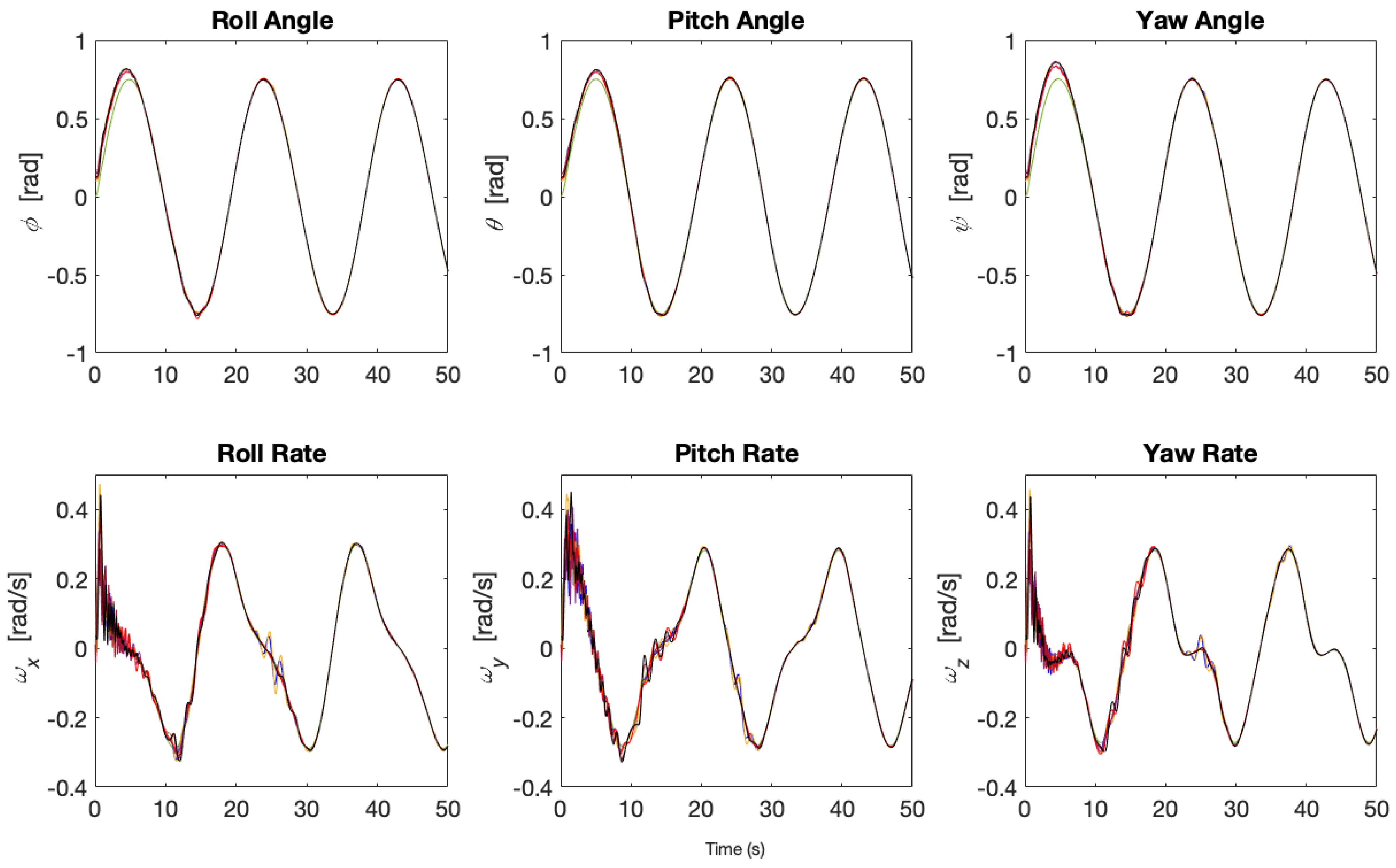
In the first case (), the synchronization of spacecraft’s states to the states of the reference can be achieved, as depicted in Figure 4. In Figure 5 and Figure 6, it can be seen that the commanded control inputs (black dashed line) exceed the actuator limit, and the actuator limits the actual control input (blue dashed line). The red dashed line is the actuator limit, , and the green dashed line is the virtual bound, . The saturation does not cause instability because the dynamics of spacecraft, which is defined in Equations (8) and (9), is a marginally stable system.
In the second case (), the synchronization of spacecraft’s states to the states of the reference can be achieved, as depicted in Figure 7. It can be observed that the control inputs do not exceed the actuator limit shown in Figure 8 and Figure 9. It can be concluded that, by choosing large enough, the synchronization problem in the presence of input constraints can be solved. Note that the large leads to the changes in reference dynamics while reducing the control deficiency. By using the reference dynamics (7), the control input, , of the leader in (8), and the commanded control input, in (18), one can verify that is proportional to the .
6. Conclusions
This work has shown the possibility to synchronize uncertain heterogeneous agents with Euler–Lagrange dynamics in the presence of input saturation. The synchronization used distributed model reference adaptive control which utilizes local states and input information and the existence distributed nonlinear matching gains between neighboring agents. Then, we proposed the adaptive control law that estimates these gains. The proposed method was modified with distributed positive mu-modification that ensure the stability of the adaptation in the presence of input saturation which requires the predecessor agent to send the control input information to the successor agent. Finally, numerical simulations of attitude control synchronization were provided to validate the proposed method. It was shown that the convergence of the dynamics can be achieved in the presence of input saturation.
Funding
This research received no external funding.
Acknowledgments
Simone Baldi from School of Mathematics, Southeast University, China, and Delft Center for Systems and Control, TU Delft, is gratefully acknowledged for useful discussions and suggestions on adaptive control.
Conflicts of Interest
The author declares no conflict of interest.
References
- Seyboth, G.S.; Ren, W.; Allgöwer, F. Cooperative control of linear multi-agent systems via distributed output regulation and transient synchronization. Automatica 2016, 68, 132–139. [Google Scholar] [CrossRef] [Green Version]
- Das, A.; Lewis, F.L. Distributed adaptive control for synchronization of unknown nonlinear networked systems. Automatica 2010, 46, 2014–2021. [Google Scholar] [CrossRef]
- Tang, Y.; Gao, H.; Zou, W.; Kurths, J. Distributed Synchronization in Networks of Agent Systems With Nonlinearities and Random Switchings. IEEE Trans. Cybern. 2013, 43, 358–370. [Google Scholar] [CrossRef] [PubMed] [Green Version]
- Olfati-Saber, R.; Fax, J.A.; Murray, R.M. Consensus and Cooperation in Networked Multi-Agent Systems. Proc. IEEE 2007, 95, 215–233. [Google Scholar] [CrossRef] [Green Version]
- Olfati-Saber, R.; Murray, R.M. Consensus problems in networks of agents with switching topology and time-delays. IEEE Trans. Autom. Control 2004, 49, 1520–1533. [Google Scholar] [CrossRef] [Green Version]
- Nazari, M.; Butcher, E.A.; Yucelen, T.; Sanyal, A.K. Decentralized Consensus Control of a Rigid-Body Spacecraft Formation with Communication Delay. J. Guid. Control Dyn. 2016, 39, 838–851. [Google Scholar] [CrossRef] [Green Version]
- Wu, Z.; Shi, P.; Su, H.; Chu, J. Exponential Synchronization of Neural Networks With Discrete and Distributed Delays Under Time-Varying Sampling. IEEE Trans. Neural Netw. Learn. Syst. 2012, 23, 1368–1376. [Google Scholar]
- Dong, H.; Wang, Z.; Gao, H. Distributed Filtering for a Class of Time-Varying Systems Over Sensor Networks With Quantization Errors and Successive Packet Dropouts. IEEE Trans. Signal Process. 2012, 60, 3164–3173. [Google Scholar] [CrossRef]
- Ren, W.; Beard, R.W.; Beard, A.W. Decentralized Scheme for Spacecraft Formation Flying via the Virtual Structure Approach. AIAA J. Guid. Control Dyn. 2003, 27, 73–82. [Google Scholar] [CrossRef]
- Lesser, V.; Tambe, M.; Ortiz, C.L. (Eds.) Distributed Sensor Networks: A Multiagent Perspective; Kluwer Academic Publishers: Norwell, MA, USA, 2003. [Google Scholar]
- Harfouch, Y.A.; Yuan, S.; Baldi, S. Adaptive control of interconnected networked systems with application to heterogeneous platooning. In Proceedings of the 2017 13th IEEE International Conference on Control Automation (ICCA), Ohrid, North Macedonia, 3–6 July 2017; pp. 212–217. [Google Scholar]
- Blaabjerg, F.; Teodorescu, R.; Liserre, M.; Timbus, A.V. Overview of Control and Grid Synchronization for Distributed Power Generation Systems. IEEE Trans. Ind. Electron. 2006, 53, 1398–1409. [Google Scholar] [CrossRef] [Green Version]
- Jun, M.; D’Andrea, R. Path Planning for Unmanned Aerial Vehicles in Uncertain and Adversarial Environments. In Cooperative Control: Models, Applications and Algorithms; Springer: Boston, MA, USA, 2003; pp. 95–110. [Google Scholar]
- Yucelen, T.; Johnson, E.N. Control of multivehicle systems in the presence of uncertain dynamics. Int. J. Control 2013, 86, 1540–1553. [Google Scholar] [CrossRef]
- Popa, D.O.; Sanderson, A.C.; Komerska, R.J.; Mupparapu, S.S.; Blidberg, D.R.; Chappel, S.G. Adaptive sampling algorithms for multiple autonomous underwater vehicles. In Proceedings of the 2004 IEEE/OES Autonomous Underwater Vehicles, Sebasco, ME, USA, 17–18 June 2004; pp. 108–118. [Google Scholar]
- Jin, X.; Haddad, W.M.; Yucelen, T. An Adaptive Control Architecture for Mitigating Sensor and Actuator Attacks in Cyber-Physical Systems. IEEE Trans. Autom. Control 2017, 62, 6058–6064. [Google Scholar] [CrossRef]
- Fax, J.A.; Murray, R.M. Information flow and cooperative control of vehicle formations. IEEE Trans. Autom. Control 2004, 49, 1465–1476. [Google Scholar] [CrossRef] [Green Version]
- Zhang, D.; Wei, B. A review on model reference adaptive control of robotic manipulators. Annu. Rev. Control 2017, 43, 188–198. [Google Scholar] [CrossRef]
- Baldi, S.; Frasca, P. Adaptive synchronization of unknown heterogeneous agents: An adaptive virtual model reference approach. J. Frankl. Inst. 2019, 356, 935–955. [Google Scholar] [CrossRef] [Green Version]
- Rosa, M.R. Adaptive Synchronization for Heterogeneous Multi-Agent Systems with Switching Topologies. Machines 2018, 6, 7. [Google Scholar] [CrossRef] [Green Version]
- Baldi, S.; Rosa, M.R.; Frasca, P. Adaptive state-feedback synchronization with distributed input: The cyclic case. In Proceedings of the 7th IFAC Workshop on Distributed Estimation and Control in Networked Systems (NecSys18), Groningen, The Netherlands, 27–28 August 2018. [Google Scholar]
- Rosa, M.R.; Baldi, S.; Wang, X.; Lv, M.; Yu, W. Adaptive hierarchical formation control for uncertain Euler–Lagrange systems using distributed inverse dynamics. Eur. J. Control 2019, 48, 52–65. [Google Scholar] [CrossRef]
- Abdessameud, A.; Polushin, I.G.; Tayebi, A. Synchronization of Heterogeneous Euler–Lagrange Systems with Time Delays and Intermittent Information Exchange. IFAC Proc. Vol. 2014, 47, 1971–1976. [Google Scholar] [CrossRef] [Green Version]
- Abdessameud, A.; Tayebi, A.; Polushin, I.G. On the leader–follower synchronization of Euler–Lagrange systems. In Proceedings of the 2015 54th IEEE Conference on Decision and Control (CDC), Osaka, Japan, 15–18 December 2015; pp. 1054–1059. [Google Scholar]
- Abdessameud, A.; Tayebi, A.; Polushin, I.G. Leader–Follower Synchronization of Euler–Lagrange Systems With Time-Varying Leader Trajectory and Constrained Discrete-Time Communication. IEEE Trans. Autom. Control 2017, 62, 2539–2545. [Google Scholar] [CrossRef]
- Baldi, S.; Rosa, M.R.; Frasca, P.; Kosmatopoulos, E.B. Platooning merging maneuvers in the presence of parametric uncertainty. In Proceedings of the 7th IFAC Workshop on Distributed Estimation and Control in Networked Systems (NecSys18), Groningen, The Netherlands, 27–28 August 2018. [Google Scholar]
- Karason, S.P.; Annaswamy, A.M. Adaptive control in the presence of input constraints. IEEE Trans. Autom. Control 1994, 39, 2325–2330. [Google Scholar] [CrossRef]
- Wen, C.; Zhou, J.; Liu, Z.; Su, H. Robust Adaptive Control of Uncertain Nonlinear Systems in the Presence of Input Saturation and External Disturbance. IEEE Trans. Autom. Control 2011, 56, 1672–1678. [Google Scholar] [CrossRef]
- Lavretsky, E.; Hovakimyan, N. Stable adaptation in the presence of input constraints. Syst. Control Lett. 2007, 56, 722–729. [Google Scholar] [CrossRef]
- Baldi, S.; Liu, D.; Jain, V.; Yu, W. Establishing Platoons of Bidirectional Cooperative Vehicles With Engine Limits and Uncertain Dynamics. IEEE Trans. Intell. Transp. Syst. 2020, 1–13. [Google Scholar] [CrossRef]
- Ortega, R.; Spong, M.W. Adaptive motion control of rigid robots: A tutorial. Automatica 1989, 25, 877–888. [Google Scholar] [CrossRef]
- Mei, J.; Ren, W.; Ma, G. Distributed Coordinated Tracking With a Dynamic Leader for Multiple Euler-Lagrange Systems. IEEE Trans. Autom. Control 2011, 56, 1415–1421. [Google Scholar] [CrossRef]
- Nuno, E.; Ortega, R.; Basanez, L.; Hill, D. Synchronization of Networks of Nonidentical Euler-Lagrange Systems With Uncertain Parameters and Communication Delays. IEEE Trans. Autom. Control 2011, 56, 935–941. [Google Scholar] [CrossRef]
- Chen, F.; Feng, G.; Liu, L.; Ren, W. Distributed Average Tracking of Networked Euler-Lagrange Systems. IEEE Trans. Autom. Control 2015, 60, 547–552. [Google Scholar] [CrossRef]
- Klotz, J.R.; Kan, Z.; Shea, J.M.; Pasiliao, E.L.; Dixon, W.E. Asymptotic Synchronization of a Leader–Follower Network of Uncertain Euler-Lagrange Systems. IEEE Trans. Control Netw. Syst. 2015, 2, 174–182. [Google Scholar] [CrossRef]
- Roy, S.; Roy, S.B.; Kar, I.N. Adaptive–Robust Control of Euler–Lagrange Systems With Linearly Parametrizable Uncertainty Bound. IEEE Trans. Control Syst. Technol. 2018, 26, 1842–1850. [Google Scholar] [CrossRef] [Green Version]
- Roy, S.; Kar, I.N.; Lee, J.; Jin, M. Adaptive-Robust Time-Delay Control for a Class of Uncertain Euler–Lagrange Systems. IEEE Trans. Ind. Electron. 2017, 64, 7109–7119. [Google Scholar] [CrossRef]
- Roy, S.; Kar, I.N.; Lee, J.; Tsagarakis, N.G.; Caldwell, D.G. Adaptive-Robust Control of a Class of EL Systems With Parametric Variations Using Artificially Delayed Input and Position Feedback. IEEE Trans. Control Syst. Technol. 2019, 27, 603–615. [Google Scholar] [CrossRef] [Green Version]
- Roy, S.; Kar, I.N.; Lee, J. Toward Position-Only Time-Delayed Control for Uncertain Euler–Lagrange Systems: Experiments on Wheeled Mobile Robots. IEEE Robot. Autom. Lett. 2017, 2, 1925–1932. [Google Scholar] [CrossRef]
- Johansen, T.A.; Fossen, T.I. Control allocation—A survey. Automatica 2013, 49, 1087–1103. [Google Scholar] [CrossRef] [Green Version]
- Ioannou, P.; Fidan, B. Adaptive Control Tutorial (Advances in Design and Control); Society for Industrial and Applied Mathematics: Philadelphia, PA, USA, 2006. [Google Scholar]
- Tao, G. Adaptive Control Design and Analysis (Adaptive and Learning Systems for Signal Processing, Communications and Control Series); John Wiley & Sons, Inc.: New York, NY, USA, 2003. [Google Scholar]
- Leonessa, A.; Haddad, W.M.; Hayakawa, T.; Morel, Y. Adaptive control for nonlinear uncertain systems with actuator amplitude and rate saturation constraints. Int. J. Adapt. Control Signal Process. 2009, 23, 73–96. [Google Scholar] [CrossRef] [Green Version]
- Romdlony, M.Z.; Jayawardhana, B. Stabilization with guaranteed safety using Control Lyapunov–Barrier Function. Automatica 2016, 66, 39–47. [Google Scholar] [CrossRef]
- Yucelen, T.; Haddad, W.M. Low-Frequency Learning and Fast Adaptation in Model Reference Adaptive Control. IEEE Trans. Autom. Control 2013, 58, 1080–1085. [Google Scholar] [CrossRef]
Figure 1.
Communication graph of multi-agent system.

Figure 2.
The body frame of spacecraft.

Figure 3.
Communication graph of multi-agent system.

Figure 4.
Adaptive spacecraft state synchronization for states () ().

Figure 5.
Control input of the leaders (blue is the actual control input and black is the commanded control input) ().
Figure 5.
Control input of the leaders (blue is the actual control input and black is the commanded control input) ().

Figure 6.
Control input of the followers (blue is the actual control input and black is the commanded control input) ().
Figure 6.
Control input of the followers (blue is the actual control input and black is the commanded control input) ().

Figure 7.
Adaptive spacecraft state synchronization for states () ().

Figure 8.
Control input of the leaders (blue is the actual control input) ().

Figure 9.
Control input of the followers (blue is the actual control input) ().


Table 1.
Satellite parameters and initial conditions.
| Initial Cond. []’ (0) | Initial Cond. []’ (0) | Moment of Inertia (kg m) | |
|---|---|---|---|
| Agent 0 (Trajectory Generator) | [0, 0, 0]’ | [0, 0, 0]’ | |
| Agent 1 (Leader 1) | [0.1, 0.1, 0.1]’ | [0.1, 0.1, 0.1]’ | |
| Agent 1 (Leader 2) | [0.3, 0.3, 0.3]’ | [−0.2, −0.2, −0.2]’ | |
| Agent 1 (Leader 3) | [−0.3, −0.3, −0.3]’ | [0.2, 0.2, 0.2]’ | |
| Agent 4 (Follower 1) | [0.2, 0.2, 0.2]’ | [−0.1, −0.1, −0.1]’ | |
| Agent 5 (Follower 2) | [−0.2, −0.2, −0.2]’ | [0.2, 0.2, 0.2]’ | |
| Agent 6 (Follower 3) | [0.4, 0.4, 0.4]’ | [0.1, 0.1, 0.1]’ |
© 2020 by the author. Licensee MDPI, Basel, Switzerland. This article is an open access article distributed under the terms and conditions of the Creative Commons Attribution (CC BY) license (http://creativecommons.org/licenses/by/4.0/).
Share and Cite
MDPI and ACS Style
Rosa, M.R. Leader–Follower Synchronization of Uncertain Euler–Lagrange Dynamics with Input Constraints. Aerospace 2020, 7, 127. https://doi.org/10.3390/aerospace7090127
AMA Style
Rosa MR. Leader–Follower Synchronization of Uncertain Euler–Lagrange Dynamics with Input Constraints. Aerospace. 2020; 7(9):127. https://doi.org/10.3390/aerospace7090127
Chicago/Turabian StyleRosa, Muhammad Ridho. 2020. "Leader–Follower Synchronization of Uncertain Euler–Lagrange Dynamics with Input Constraints" Aerospace 7, no. 9: 127. https://doi.org/10.3390/aerospace7090127
Note that from the first issue of 2016, this journal uses article numbers instead of page numbers. See further details here.