Article

3D Cruise Trajectory Optimization Inspired by a Shortest Path Algorithm

by
Alejandro Murrieta-Mendoza
,
Charles Romain
and
Ruxandra Mihaela Botez
*
Research Laboratory in Active Controls, Avionics and Aeroservoelasticity (LARCASE), Université du Québec, École de Technolgie Supérieure, Montreal, QC H3C 1K3, Canada
*
Author to whom correspondence should be addressed.
These authors contributed equally to this work.
Aerospace 2020, 7(7), 99; https://doi.org/10.3390/aerospace7070099
Submission received: 26 January 2020 / Revised: 19 May 2020 / Accepted: 2 July 2020 / Published: 21 July 2020
(This article belongs to the Special Issue Aircraft Trajectory Design and Optimization)

Abstract

:
Aircrafts require a large amount of fuel in order to generate enough power to perform a flight. That consumption causes the emission of polluting particles such as carbon dioxide, which is implicated in global warming. This paper proposes an algorithm which can provide the 3D reference trajectory that minimizes the flight costs and the fuel consumption. The proposed algorithm was conceived using the Floyd–Warshall methodology as a reference. Weather was taken into account by using forecasts provided by Weather Canada. The search space was modeled as a directional weighted graph. Fuel burn was computed using the Base of Aircraft DAta (BADA) model developed by Eurocontrol. The trajectories delivered by the developed algorithm were compared to long-haul flight plans computed by a European airliner and to as-flown trajectories obtained from Flightradar24®. The results reveal that up to 2000 kg of fuel can be reduced per flight, and flight time can be also reduced by up to 11 min.

1. Introduction

Air transportation has become an important part of the world’s economic system, as it is one of the most common means of traveling long distances and a safe way to transport valuable and perishable cargo. This has led to a continuous increase of air traffic. Naturally, this increase has created a significant rise in the demand for fossil fuels [1]. Burning fossil fuel releases polluting particles as gases; especially nitrogen oxides (NOx) and carbon dioxide (CO2). The former is known to deplete the ozone layer, and the latter is known to contribute to global warming. It is also believed that CO2 has caused wind pattern alterations, making the round trip between America and Europe longer than before, thus requiring more fuel [2]. It has been estimated that the aeronautical industry is responsible for 2% of the global CO2 released to the atmosphere [3].
The aeronautical industry has proposed its own goals to reduce air pollution. To meet these goals, different technologies have been explored within the aircraft themselves, such as lighter materials, more efficient engines, improved aerodynamics, and better aerodynamic modeling; all contributing to reducing fuel consumption and thus polluting emissions. Airlines have also implemented procedures such as washing engines, one-engine taxiing, and reducing the Auxiliary Power Unit (APU) when on the ground to reduce fuel consumption [4]. Flight operations have also been investigated and improved in order to reduce fuel consumption. Two interesting navigation examples that have reduced fuel are the Continuous Descent Approach/Operations (CDA/CDO) and the Required Navigation Precision (RNP) approach.
The CDA is a procedure in which the aircraft descends while setting engines at lowest power/lowest consumption (IDLE). Savings of 2 million gallons of fuel have been reported in Los Angeles per year [5] and of 36 gallons of fuel per flight in Atlanta [6]. The Top of Descent (ToD) coordinates must be computed correctly [7,8] while executing this procedure in order to avoid complications and the resulting need to execute further procedures such as missed approach, which are expensive in fuel burn terms as well as being costly in time and the associated airport complications [9,10].
In the terminal maneuvering area, efforts have been conducted to find the optimal landing aircraft sequence to reduce fuel burn using deterministic algorithms, metaheuristic algorithms and a combination of both [11,12,13].
Satellite navigation systems such as GPS have allowed aircraft to fly very accurate 3D routes (latitude, longitude, and altitude). These systems have allowed aircraft to fly closer to hazardous zones such as at lower altitudes and closer to mountains instead of flying long distances to fly around them. The developed RNP approach trajectories have reduced fuel consumption by up to 800 lb. per flight in Oslo [14]. The recorded savings in Kelowna were of 265,000 L per flight per year [15].
The successes of the CDA and the RNP studies show the potential advantages of providing aircrafts with a fuel-efficient trajectory. These fuel-efficient trajectories must be computed both before and during flight. Current Air Traffic Management (ATM) systems require aircraft to fly at segments of constant Mach number, at constant altitudes and following a pre-defined horizontal trajectory (or ground track). Flight trajectories must be authorized by ATM before takeoff and can be modified subsequently after a vocal clearance by ATC. This authorization is required in order to ensure separation between aircraft. However, ATC is reaching its maximum traffic capacity, and more aircrafts are expected to join the current ones. Development in Asia and Latin America suggest an increase of air traffic in the next few years. To meet this increasing demand, new systems such as NextGEN (https://www.faa.gov/nextgen/) in North America and SESARS (http://www.sesarju.eu/) in Europe are being developed to increase traffic capacity and improve safety. These new systems may allow aircrafts to automatically negotiate and move freely within the airspace, a flight mode called free flight.
A number of algorithms have been developed to find the most economical aircraft trajectory. Lovegren showed the importance of computing the optimal cruise speed and the optimal aircraft altitude; that same work also analyzed the effects of step climbs during cruise [16]. Later studies based on that work proved that commercial flights over the continental United States and inter-continental commercial flights do not take place at their optimal altitudes and speeds [17,18,19]. Another study indicated that domestic flights within Turkish airspace loaded unnecessary weight, which led to an increase of fuel flow and thus added to the fuel consumption [20]. These studies served to highlight the need to develop trajectory optimization algorithms to reduce fuel consumption.
Franco and Rivas developed an algorithm able to compute the optimal speeds for fixed cruise altitudes by taking into account a Required Time of Arrival (RTA) constraint [21]. The algorithm proposed in [22] found a path in the horizontal (ground track) dimension, as well as the most convenient fixed cruise altitudes that avoid the formation of contrails. Contrails are formations of clouds due to engine exhaust combined with water vapor, and humidity. Contrails are believed to be at least as harmful to the environment as CO2. For this reason, it is important to take contrails formation zones avoidance on the optimal trajectory problem [23]. Another algorithm designed to achieve a compromise between contrail formation and optimal fuel trajectories was developed in [24]. Rosenow et al. developed a 3D trajectory optimization algorithm that reduced CO2 and NOx emissions taking into account the airline network [25].
Using a numerical performance model with pre-defined sets of speeds and altitudes, an algorithm able to compute the optimal fixed cruise altitude and speed was developed in [26]. Felix-Patron implemented the golden section search algorithm to find, within a pre-defined set of altitudes, the optimal altitude that reduced the fuel consumption for short haul flights [27]. Dynamic programming was implemented by Hagelauer et al. and Yoshikazu et al. in order to find the most economical trajectory by changing the aircraft heading and altitude during the cruise phase while imposing time constraints [28,29]. In [30], following a realistic commercial flight and by taking into account different flight zones, flights were optimized in the horizontal dimension by taking into account wind and using a mixed integer nonlinear programming. Using that same technique, Valenzuela et al. [31] optimized an aircraft trajectory by following current airspace constraints such as constant altitude segments and constant speed.
In a similar way, Murrieta et al. [32] implemented Dijkstra’s algorithm to find the optimal lateral trajectory while taking winds into account. Murrieta et al. [33] also used that algorithm to find the best waypoints in the lateral and vertical dimensions to reduce fuel burn. Félix-Patron et al. [34] used Genetic Algorithms to optimize the lateral trajectory. Algorithms [27,28,29] were developed using a numerical performance model. Murrieta and Botez [35] proposed an algorithm to compute the flight cost using such a model. Ng et al. in [36] developed an algorithm that found the optimal trajectory by using good horizontal trajectories and executing step climbs over those horizontal trajectories. In a similar way, Félix-Patron and Botez [37] optimized the flight trajectory in its horizontal and vertical dimensions at constant speed using Genetic Algorithms; subsequently, speed was also varied to find the optimal set of speeds on which the vertical and horizontal trajectory should be flown [38].
Using hybrid optimal control, Franco and Rivas [39] optimized the trajectory by taking into account different phases of flight such as climb, cruise and descent over a pre-defined ground track. Murrieta et al. [40,41] used a beam search algorithm to find the optimal trajectory by taking also into account climb, cruise and descent phases.
Aircraft speed plays an important role in reducing fuel consumption. A study performed by Filippone showed that an aircraft normally should reduce its speed as its weight decreases [42]. Lovegren computed different speeds to reduce fuel burn during the cruise phase [16]. Murrieta et al. implemented an algorithm based on the Ant Colony Optimization methodology [43] to select the optimal combination of Mach numbers from a given set in order to fulfill am RTA constraint for a constant altitude algorithm. Murrieta et al. developed an algorithm based on the Artificial Bee Colony and Particle Swarm Optimization (PSO) in order to find the optimal trajectory on the lateral and vertical reference trajectories while fulfilling an RTA constraint [44,45]. Optimal control was used as the base of an algorithm designed to be used in a Flight Management System (FMS) to find the optimal Mach number [46]. Rosenow et al. developed an optimization algorithm, which adapts the optimal lateral route to existent ground navaids infrastructure to allow existing aircraft the Area Navigation (RNAV) implementation [47].
Although there are many different algorithms that have provided good results for the aircraft trajectory optimization problem, there are still many more algorithms that remain to be explored for aircraft trajectory on cruise phase and that could potentially provide good results. One of these algorithms is the Floyd–Warshall. The new algorithm proposed in this paper has the particularity that it simultaneously optimizes the vertical and the lateral reference trajectories instead of optimizing the lateral first, and then the vertical trajectory as t is normally done in the literature. This paper as well shows a way to deal with the different weights of the aircraft coming from different edges to a given waypoint.
A new algorithm is proposed in this paper to find an economical flight trajectory for a commercial aircraft. This proposed algorithm was inspired by the Floyd–Warshall algorithm, especially because it is a deterministic algorithm, meaning that it will always provide the same output for the same inputs. Moreover, the Floyd–Warshall algorithm enables to trace back its decisions. For this reason, the developed algorithm could potentially be loaded onto in-flight avionics systems such as the FMS, unlike the metaheuristic and heuristic algorithms based on random decisions. Its characteristics are very desirable, as they are fundamental for the avionics certification process. This paper has two main goals: 1) to find the optimal (most economical) trajectory in terms of flight cost, and 2) to analyze and validate that the provided trajectories are feasible.
This paper is organized as follows. In Section 2, the aircraft, search space, the fuel burn, and the weather models are explained. The proposed optimization algorithm is described in Section 3. Section 4 presents the results obtained, and then the paper ends with the conclusions and recommendations for future work.

2. Aircraft, Search Space, Fuel Burn, and Weather Models

2.1. Aircraft Model

The aircraft model selected for this work was the point mass approach. This 3 Degrees of Freedom (DOF) model is derived from aerodynamics and Newtonians laws. The performance characteristics, and especially the fuel burn, are computed using the Base of Aircraft DAta (BADA) model developed by Eurocontrol [48].
The aircraft equations of motion used here are those developed in [49]. They consider that the aircraft is a point of mass, the Earth is flat and non-rotational, gravity is constant, aircraft mass is not a state variable, thrust force is aligned with airspeed, there is no side slip, and path angle changes are assumed to be instantaneous. These considerations lead to the use of simplified equations. This model is also known as the gamma-command model, and is defined in Equations (1)–(6):
V ˙ T A S = T h r u s t D m g s i n γ T A S m w ˙ X d
χ ˙ H D G = 1 V T A S c o s γ T A S ( L s i n μ T A S m w ˙ Y d )
L c o s μ T A S m g c o s γ T A S + m w ˙ Z d = 0
φ ˙ = V T A S c o s γ T A S s i n χ H D G + v R M + h
λ ˙ = V T A S c o s γ T A S c o s χ H D G + u R M + h
h ˙ = V T A S s i n γ T A S + w
where λ and φ represent the aircraft longitude and latitude, respectively, h is the altitude; χHDG is the aircraft heading, γ is the pitch, µ is the roll, and m is the aircraft’s mass. The variables wd, Yd, and zd represent the wind rate parallel to the aircraft, parallel to the Earth’s surface and perpendicular to the aircraft, respectively, and u, v, and w indicate the west, south, and vertical winds, respectively. Finally, L is the lift. This last coefficient is computed using BADA, and is a function of the in-flight conditions.
All these equations of motion are provided for completeness. As the distance between two waypoints is small enough (a maximum of 150 Nautical Miles-NM), it is considered that the heading is kept constant while flying between two waypoints. Therefore, updating the heading state is not required while flying between two waypoints. Distance is computed using the waypoints’ geographical position (latitude, longitude) and the Vincenty’s formulae [50].

2.2. Weather Model

Wind information is given in the form of a forecast called the Global Deterministic Forecast System (GDPS) provided by Environment Canada. This forecast dataset provides the world’s weather forecast on a 601 × 301 latitude-longitude grid at a resolution of 0.6° × 0.6° every 3 h (0 h, 3 h, 9 h, …, 144 h), and at different pressure altitudes. Every point of the grid contains weather information. Among the data provided by this forecast model, only the Wind Angle, Wind Speed, and Temperature are of interest for the proposed algorithm.
The weather information for the aircraft’s exact geographical position, time, and altitude is computed using the following procedure:
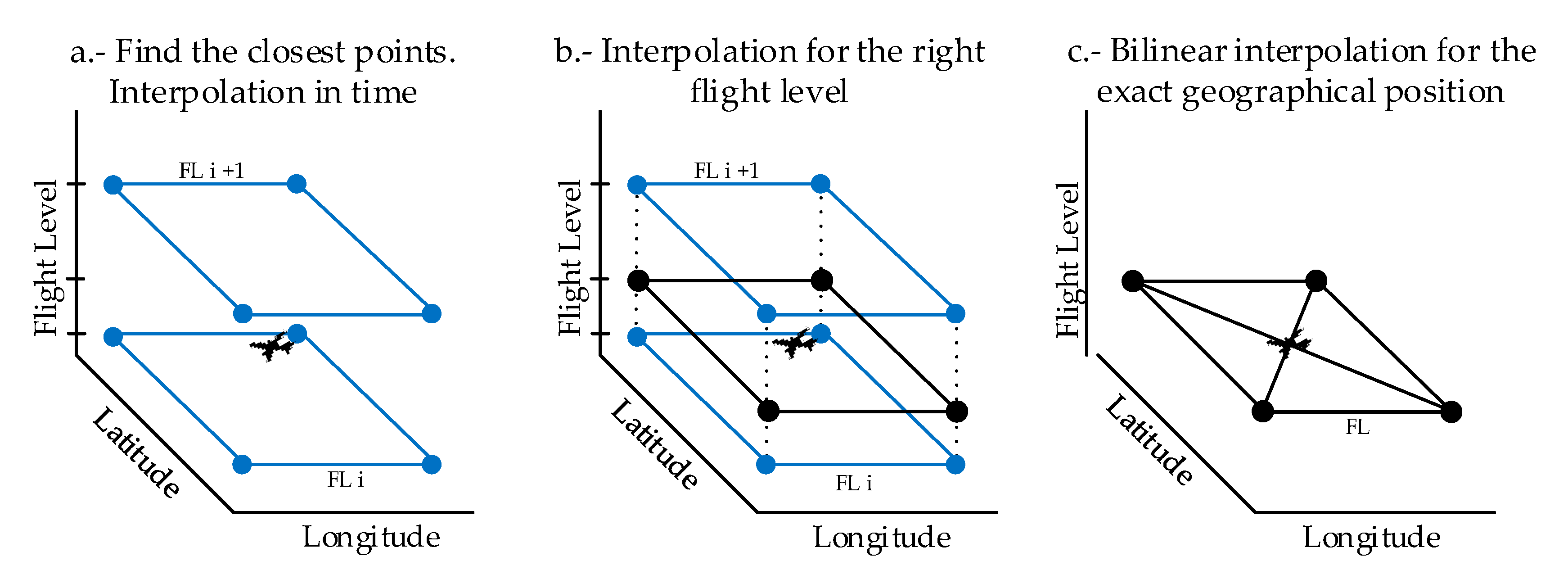
  • Identify the four GDPS’s grid points surrounding the aircraft during the flight performance computation. In other words, not only at the waypoints;
  • Determine the pressure altitude for the current aircraft’s flight level;
  • Identify the immediate higher and lower pressures from the aircraft’s flight level from the GDPS forecast. For example, at 35,000 ft, the pressure is 230 hPa, and so the lower and higher available pressures would be 225 hPa and 250 hPa, respectively;
  • Using the GDPS forecast, identify the immediate higher and lower time blocks from the current time. (For example, if the current time is 14 h 35 m, the lower and higher time blocks would be 12 h and 15 h, respectively, thus interpolations are executed for 14 h 35 m with these two limits.);
  • Perform temporal linear Lagrange interpolations for the lower and higher pressure altitudes for the 4 points surrounding the aircraft, as shown in Figure 1a;
  • Perform linear Lagrange interpolations in pressure levels (flight level) for the 4 points surrounding the aircraft, as indicated in Figure 1 and Figure 2 After executing these interpolations, the weather is known for the exact pressure altitude at the current time for the 4 points surrounding the aircraft; and
  • Perform bilinear interpolations using the 4 points surrounding the aircraft to obtain the weather information at the aircraft’s position, as shown in Figure 1, Figure 2 and Figure 3.
The information obtained from the weather forecast allows the computation of different parameters, such as the local speed of sound, the Ground speed, and the International Standard Atmosphere (ISA) temperature deviation (ISAdev). These values are required to compute the fuel burn, as is explained in Section 2.3.
The local speed of sound (a) is defined in Equation (7):
a = γ   r   T ,
where γ is the air adiabatic value 1.1, r is the gas constant with a value of 286 m2/s2/K, and T is the local temperature.
The ISA temperature deviation (ISAdev) can be defined as the temperature difference between the real local temperature and the temperature provided by the ISA model (ISATEMP), as shown in Equation (8):
I S A d e v = T I S A T E M P
The Ground Speed (GS) is the aircraft speed relative to the ground. It is computed using the Wind Speed (WS) and the Wind Angle (WA) obtained from the weather forecast, the True Air Speed (TAS), and the aircraft heading, as shown in Equation (9):
G S = T A S W S ,
where
T A S = M a c h   · a ,

2.3. Search Space

Flying under the “free trajectory” concept means that the aircraft can fly anywhere within the airspace. This fact implies that there are infinite combinations of points in the space with which a trajectory can be generated. To limit the number of combinations, the search space is modeled as a unidirectional graph G(E,V), in which E denotes the links connecting two consecutive waypoints, and V are the waypoints defining the search space. The search space is created in 3D: the lateral coordinate, the longitudinal coordinate, and the altitude. This search space contains the cruise phase, defined as from the Top of Climb (ToC) to the Top of Descent (ToD) coordinates. Trajectories are generated from the ToC, and they end at any waypoint at the ToD. This search space is generated using a reference trajectory, which can be a great circle (geodesic) trajectory or a real trajectory obtained either from flight plans or historical flights via such sources as Flightaware® or Flightradar24®. The separation between the ToC and the two first waypoints in the lateral dimension was arbitrarily set to 7.5°, a value that was assumed large enough to avoid sudden pronounced heading changes. A large angle would place the adjacent waypoints too from each other by creating a larger distance among waypoints. In this case, the effect of wind might not be enough to compensate for this extra distance. A too small deviation angle might place the waypoints too close to each other, which would mean that weather remains practically the same within the search space. For this reason, the aircraft might follow the central waypoints as there would be no advantage of changing waypoints. Altitudes can only be flown at 1000 ft multiples. As stated before, the distance between to waypoints is the geodesic computed using the Vincenty’s formulae. The search space is illustrated in Figure 2.
Figure 2 shows the ToC at the initial cruise altitude in green, and the possible ToDs in orange. The path created by the line crossing waypoints 1-4-14-27-35 is the lateral and longitudinal reference trajectory at constant altitude. All the other waypoints are placed using this path as reference. The red lines show examples of different alternatives to get from waypoint 1 to intermediate waypoint 15.

2.4. Fuel Burn Model

Only the cruise phase is taken into account in the proposed algorithm. During this phase, the aircraft is normally flying at a constant altitude and at a constant Mach number. However, the aircraft is able to perform changes of altitudes, either climbing to a different flight level (step climb), or descending to another flight level (step descent).

2.4.1. Fuel Burn Model in the Cruise Phase

The fuel burn model is computed based on a steady cruise flight where the generated lift is equal to the aircraft’s weight (Equation (3)). As shown in the BADA model, the lift coefficient (CL) is computed with Equation (11).
C L = 2   ·   m   ·   g o p   ·   γ   ·   S r e f   ·   M a c h ² ,
This CL is introduced in a polynomial provided by the BADA model, which in turns provides the drag coefficient (CD) that allows the drag to be computed for the given flight condition with Equation (12).
D r a g = p · γ · S r e f · M a c h ² 2 · C D ,
As for a flight in equilibrium, thrust equals drag, and so the thrust coefficient (Ct) required to compute the fuel burn is given by Equation (13).
C t = T h r u s t p p o · M r e f · g 0 ,
This thrust coefficient (Ct) is also introduced in another BADA polynomial, which in turn provides the fuel coefficient (Cf). Fuel flow can then be computed with Equation (14).
f u e l   f l o w = p p 0 · ( t t 0 ) 1 2 · M r e f · g 0 · a 0 L h v C f ,
where Lhv is the lower heating value of the aircraft and Mref is the aircraft’s reference mass defined by the BADA model times g0.
While computing the fuel burn in cruise, the algorithm divides the distance between two waypoints in 25 nm sub-segments (and a smaller one if the total distance is not a multiple of 25 NM). At each sub-segment, the weather is obtained and the fuel burned is reduced from the aircraft’s total mass. This is done in order to improve accuracy. A distance of 25 NM was selected as it is a good compromise between fuel burn accuracy and computation time. When the aircraft changes level, the edge’s cost consist of the change level cost plus the cost of flying at the new level until the next waypoint.

2.4.2. Fuel Burn Model for Climb and Descent during Cruise

When the aircraft climbs to a different flight level, it is assumed that the throttle is set to the maximum climb position (MCMB), and that it is set at IDLE for descent.
When performing step climes (or descents) during the cruise phase, the aircraft steadily gains altitude without performing sudden path angle changes. It can also be assumed that steady climbs present small path angle variations. For this reason, CL, CD, and D can be computed with Equation (11) and Equation (12) as if it was a steady cruise. The Thrust for the aircraft configuration is computed using Equation (15):
T h r u s t C L B = C t m c m b · p p 0 · m ,
where m is the aircraft grossweight, Ctmcmb is computed using a polynomial provided by BADA. Cf is once again computed using the BADA polynomial, but as a function of Ctmcm. Fuel flow for the climb phase is computed using Equation (14).
Having computed ThrustCLB and D, the Rate of Climb/Descent (ROCD) can be computed using Equation (16).
R O C D = t · ( T h D ) · T A S · t 2 · m · g 0 ,
where t is the temperature at the actual altitude, t2 is the temperature at the targeted altitude, ThrustCLB is the thrust during climb, D is the drag, fm is the energy factor, and g0 is the gravitational constant (9.81 m/s2). The ROCD is used to track the targeted altitude, which is done as follows:
  • The Flight Time for a given horizontal distance is computed using the GS. This horizontal distance, although it changes depending on the distance between two waypoints, is generally around 25 NM.
  • The ROCD is computed using Equation (16).
  • The current altitude is computed with Equation (17).
    A l t i t u d e ( i t e r a t i o n ) = A l t i t u d e ( i t e r a t i o n 1 ) + R O C · F l i g h t T i m e ,
  • If the resulting Altitude (iteration) is equal to or higher than the targeted altitude, the algorithm computes the fuel burn as in the cruise phase (Section 2.4.1). Otherwise, the next distance is selected, and the procedure continues again at step 1.
As a result that the horizontal distance is small enough, if the Altitude value overshoots the targeted altitude by a few tens of feet, the cruise phase is rounded to the closest 1000 ft altitude.
The way the graph is designed, it allows only for a climb or a cruise per waypoint. For this reason, when the fuel burn is computed for a cruise/descend, there is normally a constant cruise flight computation. The algorithm computes first the climb/descent to the target altitude. Once there, it keeps computing the flight cost following the process described for a fixed altitude cruise in Section 2.4.1.

2.5. Flight Cost Model

The typical flight cost for commercial aircraft depends on three parameters, as shown in Equation (18).
F l i g h t   C o s t ( k g ) = F u e l   B u r n ( k g ) + C I ( k g h r ) F l i g h t   T i m e ( h ) ,
where Cost Index (CI) is normally a parameter that translates the Flight Time in terms of Fuel Burn. This parameter is defined by the airline before take-off, and it remains constant through the duration of flight. The usual CI values are from 0 to 99 (or 999).
The CI gives priority to Fuel Burn or to Flight Time. For example, taking the CI scale from 0 to 99, a CI = 0 means that the Flight Cost gives priority only to Fuel Burn, without taking into account Flight Time. A CI = 50 would be a good compromise between Flight Burn and Flight Time. Finally, a CI = 99 gives full priority to Flight Time without caring about Fuel Burn. This means that for a set of available speeds, the CI would directly affect the aircraft speed by making a good compromise between speed, flight time cost and fuel burn (including step climbs). However, this research only uses one Mach number (speed).

3. The Optimization Algorithm

The objective of this optimization algorithm is to minimize the Flight Cost described in Equation (18). In other words, the algorithm finds the combination of waypoints that provides the most economical reference trajectory in terms of Flight Cost. To achieve this objective, the Floyd–Warshall (FW) algorithm was implemented in order to find the 3D reference trajectory optimization.

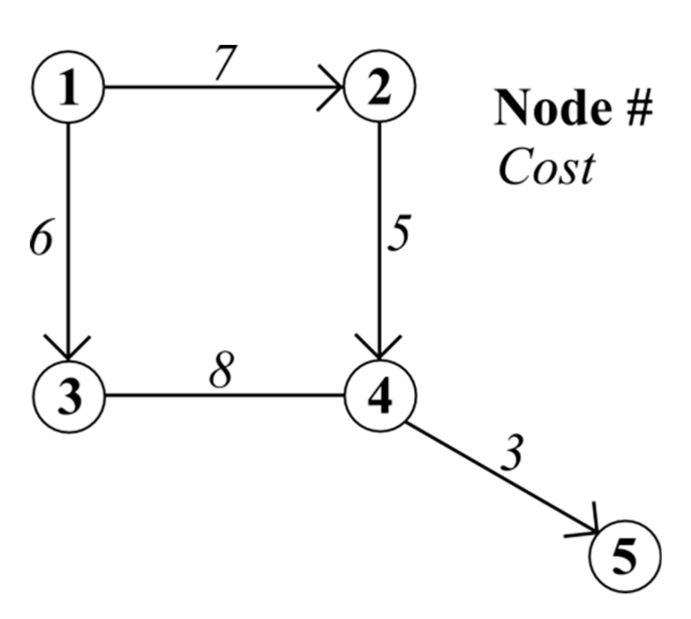
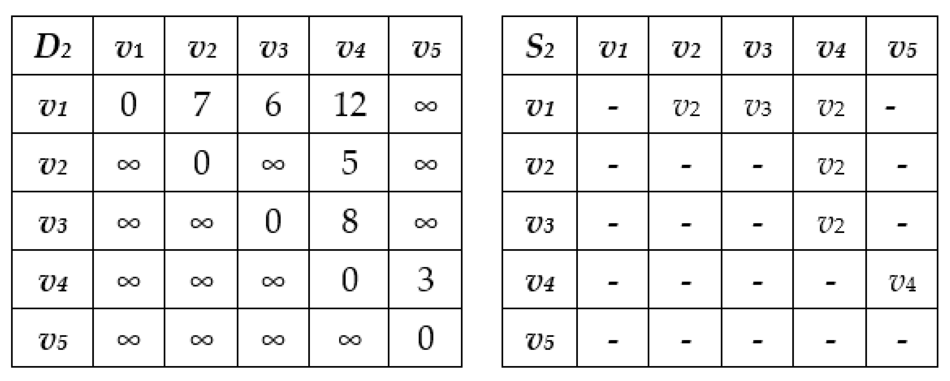
3.1. The Floyd–Warshall Algorithm

The FW optimization algorithm is based on Dynamic Programming first reported in [51,52]. This is an iterative node-to-node algorithm that finds the optimized path between all the node pairs in a given positive weighted directed graph. The FW algorithm is based on the concept that the optimal path between a vertex v0 and a vertex vf passes through the intermediate vertex vi. Thus, the sum of the weights of vertices (v0, vi) and (vi, vf) is equal to the optimal trajectory. During the execution of the algorithm, a node is selected as the intermediary node, and the optimal path between that node and two other nodes is computed. The pseudo-code for the FW algorithm is shown in Figure 3.
In Figure 3, D represents the edges’ weights, and R is the adjacent matrix that shows the directly connected vertices. This pseudo-code states that if placing the vertex k as an intermediate vertex between the vertices i and j provides a more economical cost than the direct connection of vertices i and j, then the node k is placed in the corresponding indices in the R matrix and the D matrix is updated with the new cost. In other words, each column and row represent different vertices. This algorithm takes a node vk (Figure 3—line 1) and compares the cost of interconnecting node vi and vj via node vk to the cost of the direct connection of vi to vj (Figure 3—line 4). If connecting via vk is more economical, then that cost is updated on matrix D (Figure 3—line 5), and the node vk is put on matrix S between nodes (or row i/column j) vi and vj (Figure 3—line 6). This process is repeated for all nodes among all the edges’ connections until the last iteration, at which matrices D and S provide the most economical costs and the immediate connections of all the nodes needed to obtain the optimal 3D trajectory.
For the sake of clarity, a demonstration of how the algorithm behaves is explained below step-by-step using the graph shown in Figure 4.
In the beginning of the algorithm, the matrices D0 and S0 are the following in Figure 5.
By inspection, it can be seen that the weights in matrix D0 are those of linking nodes, for example, the link v1 to v2 has a cost of 7, the link v4 to v5 has a cost of 3 and so on. Matrix S0 shows the nodes connecting any other two nodes. This can be read as follows: to get to node v2 from node v1, we should pass through v2. As this example advances, the utility of matrix S will become more evident.
At the first iteration k =1, the algorithm searches for all the nodes that v1 interconnects. As this node is the initial one, it does not help to interconnect any other two nodes (see Figure 4), no change in D and R is required, and so D1 and R1 remain with the same values as D0 and S0.
At k =2, it can be seen that node v2 interconnects nodes v1 and v4. In the algorithm, with the terms at i = 1, j = 4, and k = 2, the cost from v1 to v4 via v2 is compared to the known direct path cost between v1 and v4, as shown in Figure 3 line 4 (D1[v1][v4] > D1[v1][v2] + D1[v2][v4]). If the cost to flight via v2 is more economical than the direct cost v2v4, then the new cost is replaced by the computed one and the matrix S is updated with the vertex used to connect v1 and v4, v2 in this case. For this example, replacing these values for the numerical ones is possible as ∞ > 7 + 5. Obviously, (7 + 5) is smaller than ∞. Therefore, the path can be improved and so the cost to travel from v1 to v4 passing through v2 is added to the matrix as D2[v1][v4] = 12 and matrix S2[v1][v4] = v2. In other words, the path v1 to v4 is more economical via v2. The new matrices D2 and S2 are now as in Figure 6.
The same process is repeated until k = 4. For the last iteration k = 5 (node v5), according to the graph in Figure 4, it does not serve to interconnect any nodes, and so there is no change. Thus, matrices D4 and S4 are the same as matrices D5 and S5 in the final form.
Based on Figure 7, the most economical trajectory between v1 and v5 has a cost of 15, as shown by D5. The optimal path can be constructed using matrix S5; to get from v1 to v5, the path should pass through v4. To go from v1 to v4, the path should pass through v2, and finally, v1 to v2 is a direct path. Thus, the optimal path is v1-v2-v4-v5.

3.2. The Floyd–Warshall (FW) Algorithm for the 3D Reference Trajectory

The search space defined in Section 2.5 is a unidirectional positive weighted graph, and so the FW algorithm can be utilized to determine the 3D reference trajectory. It may be worthwhile to consider all of the waypoints in order to compute sub-optimal trajectories in case ATC requests the aircraft to change its current optimal trajectory. However, for the algorithm developed in this paper, the objective is to find the most economical trajectory between the ToC and the ToD. The ToC is the first vertex, and the ToD is the last vertex; for the rest of this paper, the word vertex will be interchanged with the word waypoint. Thus, by taking advantage of the graph structure, only the element of the first row of the matrices S and D needs to be found. In other words, the shortest path for the developed algorithm is found between the first (the first column in the first row referring to the ToC waypoint) and the last waypoints (the last columns referring to the ToD waypoints in the first row). This is expressed in the pseudo-code shown in Figure 8.
The difference in this code from the typical FW pseudo-code is that there are now only two loops (Figure 9) instead of three (Figure 3). In addition, note that Matrix R always refers to row 1 (ToC), and that in most instances, matrix D only refers to row 1. This modification dramatically reduces the computation time, as the algorithm does not loop for all nodes.
As the reference trajectory optimization algorithm evolves, the Flight Cost calculated for the segment between two waypoints is computed talking into account the aircraft weight and the weather at the time and location of the waypoint.
To solve the 3D reference trajectory problem, the algorithm must find the most economical (shortest) paths between the ToC and the nodes that are defined as the ToDs. As explained above, the algorithm uses two square matrices called S and D. S represents each waypoint and its connections with the other waypoints, while D represents the flight cost between those waypoints.
The fuel burn optimization is mostly based on the vertical optimization. Optimizing the step climb looks for the waypoint where to change cruise altitude, and thus ensures that the aircraft is flying at the optimal altitude. Lateral navigation results in saving flight time which reduces the amount of fuel burned.
Flight time optimization is based on taking advantage of the winds. It modifies both the lateral and the vertical trajectories in order to reduce the flight time using the same flight conditions (Mach numbers, pressure), thereby reducing both the time of flight and the amount of fuel burned.
Using a graph search algorithm brings the problem of tracking the aircraft weight (and other information such as the exact time, important for weather information and the flight cost computation) when two different edges connect to a given waypoint which subsequently connects to another set of waypoints. Keeping this information for all combinations is impractical as this would require high memory requirements as well as extra time required to access to the different memory slots. To improve this, the path systems is proposed.

3.3. Special Considerations for the Trajectories on the Algorithm: The Path System

The final form of a graph (E) is known. Taking the example of Figure 2, where all the possible connections from TOC to node 15 are shown, the different connections are known shown in Table 1, in which Si,j shows a direct connection between two nodes, where the cost can be directly computed if the state at the current node (first row) is known. Infinite (∞) refers to the costs to be computed. According to Figure 8 the goal of the proposed algorithm is to find the optimal trajectory from the node 1(ToC) to any other node within the graph.
The first row refers to the connections from the ToC to any other node until node 15. By inspecting Table 1, it can be seen that many cells are not used, which is causing un-necessary memory utilization. It is evident that the more nodes are in a table, the more un-necessary cells will be. For this reason, it is better to represent the connections under the form of a list, as shown in Table 2.
By comparing the number of values, Table 1 requires 255 values in memory to compute the optimal path from the ToC to node 15, while Table 2 only requires 35 values, this is a reduction of 640%. This reduction dramatically reduces the computation time, and is the main advantage of Table 2 over Table 1.
The second advantage is the way in which the values such as aircraft weight and time are treated along the trajectory. Many edges can be connected to a given node, which in turn has more edges connected to different nodes, weight and time (to determine weather information). All information for every connection between nodes is necessary to correctly compute the flight cost. However, the main interest is to find the optimal path from node 1 (ToC) to every other node in the graph. This finding allows to discard information from nodes that have been discarded as they have been determined to be non-optimal.
For example, in Table 2, indices 1 to 6 show all the connections (edges) that connect node 1 to node 8. It is convenient that the aircraft weight and the time at the first node (the ToC) are known, thus the first edge’s weights (1 to 2–6) can be computed. The optimal node connecting node 1 to node 8 is stored in index 7 (S1,8). This is the only pair weight/time information saved, all the other information (pair weight/time) for the connections (edges) leading node 1 to 8 are discarded as it refers to sub-optimal values.

3.4. The 3D Optimization Algorithm Pseudo-Code

The algorithm can be summarized as the pseudo-code in Figure 9.
In the first part of the algorithm, the flight information as well the weather information are loaded from a flight plan and from the weather forecast. Weather is required to take wind and temperature into account in order to compute the flight later. Then, the search space is created based on the flight plan. As a result of the fact that the search space has always the same shape (ToD connected to a set of waypoints, which are then connected to another set of waypoints until the ToDs are reached), the required connection tables are created. The algorithm then requires specific information such as take-off mass, Mach number, and the CI. When all this information is ready, the adapted Floyd–Warshall algorithm is implemented. At this step, the cost to fly from any waypoint i to any waypoint j taking weather into account is constantly computed. Once the Floyd–Warshall algorithm ends, the results are displayed.

4. Results

The aircraft selected to perform optimization tests is a twin-engine long haul wide body aircraft. This aircraft has a maximal takeoff weight of around 164,000 kg and a capacity of around 200 passengers. The flights were selected from two sources: flight plans provided by a major European airline and flight plans from radar data provided by Flightradar24®.

4.1. Flight Optimization from Airlines Computed Flight Plans

The first set of results aims to graphically show the optimization results on 3D for both: the vertical and the lateral reference trajectories. For this aim, a flight from Montreal to Rio de Janeiro is shown in Figure 10 for the lateral (a) and for the vertical trajectories (b). The 3D optimization for this flight represented a total saving of around 280 kg (0.82%) compared against the as “flown” flight.
In Figure 10a, the green waypoints represent the available search space for the current flight, the blue waypoints represent the followed nodes (waypoints) for an as-flown flight, and the red waypoints represent the 3D waypoints. It can be seen that for the 3D reference trajectory provided by the algorithm, the flight tends to move more Eastwards than the as-flown flight, this result could be explained by the fact that there are better wind conditions on the east than in the west side. Figure 10b show the vertical trajectory optimization where it is possible to visualize the changes of altitude of the as-flown flight (Real), the optimized vertical reference trajectory (following the blue waypoints), and the optimized 3D vertical trajectory (following the red waypoints). It can be seen that all trajectories are similar. The main difference is that the as-flown (real) trajectory has two cruise constant altitude long flight segments at 37,000 ft and at 39,000 ft of around 3000 nm each. The optimized 3D consists in a quick climb to 36,000 ft followed by a long constant cruise of around 2000 nm to execute then many step climbs until reaching 41,000 ft. The 3D vertical trajectory as well shows a short constant cruise, which could be attributed to a good combination of wind at the new flight level and the correct time to change the altitude due to the aircraft’s weight. The low optimization is attributed to similar profiles, the 3D optimized flight executes 5 step climbs, compared to the real flight. It can be seen that for the 3D optimized flight, there are two step climb at around 3000 nm executed one after the other. The fuel savings from that part of the optimized flight can be considered to be low as climbing to a different altitude is an expensive procedure in fuel burn terms. The lateral profiles are close together with their largest difference in the middle of the flight.

4.2. Flight Optimization from Airlines Computed Flight Plans

As-flown trajectories were optimized using the algorithm developed in this paper. A total of four as-flown flight plans were provided by a European airliner. The takeoff and arrival airports were Bucharest and Tenerife. The flight plans were first flown using the BADA fuel burn model. Next, the optimization algorithm was executed for the same flights in two different ways: for the vertical dimension only, and in 3D. The Mach number was 0.8, the weights were the same as t stated in the flight plans. For reasons of confidentiality, the weights and the real cost indexes cannot be provided here. As a result that the Mach number is fixed to only 0.8, the CI will not actually make any influence in the decisions taking by the algorithm. The results are shown in Figure 11 and Figure 12.
For all four flights, the flight plan provided by the airline was the most expensive flight in terms of flight cost, and three of the airline’s flight plans incurred more fuel burn. The optimized vertical flight (Vertical Opt) was able to optimize the trajectory by selecting better altitudes than the flight plan computed and flown by the airline. The trajectory provided by the optimization algorithm was able to provide a more economical flight than the computed trajectory simply by optimizing the vertical profile for three of the four flight plans.
However, the vertical trajectory optimization was more expensive than the flight plan for the 14th of July, but the flight cost was more economical. This result can be attributed to the fact that the selected altitudes are more expensive in fuel burn terms, but the winds at the vertical optimized reference trajectory made the flight faster and thus more economical in terms of flight cost.

4.3. Flight Optimization for as-Flown Flights

It is worthwhile to evaluate the optimal flights from different destinations. Therefore, different destinations were evaluated by comparing the results provided by the optimization algorithm against the as-flown flights’ flight costs. A variety of different flights were obtained from Flightradar24®; the airport codes used for the evaluated flights are listed in Table 3.
For all the tests shown in this section, the take-off weight at the ToC (the point where the cruise phase begins) was considered to be 125,000 kg, and the cost index was arbitrarily set to 50. As can be seen in Table 4, the 3D FW algorithm was able to provide more efficient fuel burn flights, as it could identify the waypoints at which to execute step climbs in order to reduce fuel burn. The algorithm was also able to guide the aircraft to zones where wind conditions were favorable for the aircraft in terms of fuel burn (see Table 4).
The average fuel burn optimization (savings) was close to 4.44%. There was an additional flight evaluated from London to Montreal, which burned a total of 32,982 kg and the optimization algorithm provided a trajectory that only required 26,802 kg of fuel (6180 kg—18.74%). This flight was not considered on the average nor on Table 2 or Table 3 because it is considered an abnormal flight, as the as-flown flight was executed following a constant fixed altitude of 30,000 ft during the flight duration. This constant fixed altitude brings as a consequence an inefficient flight. Long haul flights normally begin at low altitudes and execute step climbs during cruise. This flight serves to show the importance of providing good fuel-efficient trajectories. There are many possible explanations for why this flight was flown at this altitude, including, but not limited to bad weather, too much traffic, or ATC constraints.
Table 5 shows the comparison between the reference flights and the optimized flights in terms of flight time. It can be seen that all flights are shorter with the trajectories provided by the algorithm, as the aircrafts were guided to zones where the winds tend to reduce flight time.
Flight time is very important, as it is multiplied by the Cost Index to determine (along with the fuel burn) the overall flight cost as in Equation (18). The Cost Index for all the flights evaluated here was selected as 50. Figure 13 shows the flight costs, indicating the fuel burn parts and the flight time cost parts for the real flights (in stripes, obtained from FlightTrack24®) and the 3D FW optimized flights (in solid colors, obtained from the algorithm’s output).
By analyzing the results in Table 4 and Table 5, it can be seen that the trajectories provided by the 3D FW algorithm were more economical in terms of fuel, and that all the optimized flights were shorter. Therefore, as expected, the flight costs were always more economical for all flights.
The optimal trajectories were delivered within an average of 281 s; the longest execution time was 348 s and the shortest delivery took 217 s. These tests were performed on an AMD ® Phenom II X4 B93 processor at 2.80 GHz.

5. Conclusions

The Floyd–Warshall algorithm was able to optimize the fuel consumption during the cruise phase on long haul flights by selecting the waypoints where step climbs were executed, and by modifying the aircraft heading to guide it to zones where winds tended to be tailwinds. The search space was modeled in the form of a weighted graph which allowed the implementation of a dynamic programming-based algorithm.
The reduction of fuel burn and flight cost are helpful in reducing the pollution released to the atmosphere, which could achieve the aeronautical industry’s environmental goals in green aircraft technology. The flight cost reductions could also lead to increase the airlines’ profits.
The deterministic nature of this algorithm allows it to be possible to be implemented in current avionic devices such as the Flight Management System. The execution time is considered to be low; however, it would be desirable to reduce this execution time even further in order to be able to implement the algorithm in avionics systems that normally have limited power resources.
Improving this algorithm will allow it to fulfill the Required Time of Arrival (RTA) constraint, which is key to future airspace systems. The Floyd–Warshall algorithm is able to provide the shortest path between any two points. The algorithm presented in this paper only keeps the trajectory between two points, the ToC to the ToD, in its memory. It would be advantageous to enable this algorithm to hold many more waypoints and thereby allow an aircraft to fly to any waypoint if air traffic control requests a change of trajectory.

Author Contributions

Conceptualization, A.M.-M.; Methodology, A.M.-M. and C.R.; Validation, A.M.-M. and C.R.; Formal Analysis, A.M.-M. and C.R.; Resources, R.M.B.; Data Curation, C.R.; Writing-Original Draft Preparation, A.M.-M. and C.R.; Writing-Review & Editing, A.M.-M. and R.M.B.; Visualization, C.R.; Supervision, R.M.B.; Project Administration, R.M.B.; Funding, R.M.B. All authors have read and agreed to the published version of the manuscript.

Funding

This research received no external funding.

Acknowledgments

We would like to thank the team of the Business-led Network of Centers of Excellence Green Aviation Research & Development Network (GARDN), and in particular Sylvan Cofsky for sponsoring this project (GARDN II – Project: CMC-21). This research was conducted at the Research Laboratory in Active Controls, Avionics and Aeroservoelasticity (LARCASE) in the framework of the global project “Optimized Descent and Cruise”. For more information please visit http://larcase.etsmtl.ca. We would like to thank Rex Haygate, Dominique Labour, Oussama Abdul-Baki, Reza Neshat and Yvan Blondeau from CMC-Electronics – Esterline, TAROM airlines for the provided flight plans, and Oscar Carranza from LARCASE for their invaluable contributions. We also would like to thank the FQRNT.

Conflicts of Interest

The authors declare no conflict of interest in this work.

References

  1. ATAG. Aviation Benefits Beyond Borders; Air Transport Action Group: Geneva, Switzerland, 2016; p. 80. [Google Scholar]
  2. Williams, P.D. Transatlantic flight times and climate change. Environ. Res. Lett. 2016, 11, 024008. [Google Scholar] [CrossRef]
  3. ICAO. Aviation’s Contribution to Climate Change; International Civil Aviation Organization: Montreal, QC, Canada, 2010; p. 260. [Google Scholar]
  4. McConnachie, D.; Wollersheim, C.; Hansman, R.J. The impact of fuel price on airline fuel efficiency and operations. In Proceedings of the 2013 Aviation Technology, Integration, and Operations Conference, Los Angeles, CA, USA, 12–14 August 2013. [Google Scholar]
  5. Clarke, J.P.; Brooks, J.; Nagle, G.; Scacchioli, A.; White, W.; Liu, S.R. Optimized profile descent arrivals at los angeles international airport. J. Aircr. 2013, 50, 360–369. [Google Scholar] [CrossRef]
  6. Kwok-On, T.; Anthony, W.; John, B. Continuous descent approach procedure development for noise abatement tests at louisville international airport, KY. In Proceedings of the AIAA’s 3rd Annual Aviation Technology, Integration, and Operations (ATIO) Forum, Denver, CO, USA, 17–19 November 2003. [Google Scholar]
  7. Johnson, C.M. Analysis of top of descent (tod) uncertainty. In Proceedings of the 2011 IEEE/AIAA 30th Digital Avionics Systems Conference (DASC), Seattle, WA, USA, 16–20 October 2011; pp. 2E3-1–2E3-10. [Google Scholar]
  8. Stell, L. Predictability of top of descent location for operational idle-thrust descents. In Proceedings of the 10th AIAA Aviation Technology, Integration, and Operations (ATIO) Conference, Fort Worth, TX, USA, 13–15 September 2010. [Google Scholar]
  9. Murrieta-Mendoza, A.; Botez, R.M.; Ford, S. New method to compute the missed approach fuel consumption and its emissions. Aeronaut. J. 2016, 120, 18. [Google Scholar]
  10. Dancila, R.; Botez, R.M.; Ford, S. Fuel burn and emissions evaluation for a missed approach procedure performed by a b737-400. Aeronaut. J. 2014, 118, 20. [Google Scholar] [CrossRef]
  11. Samà, M.; D’Ariano, A.; Corman, F.; Pacciarelli, D. Metaheuristics for efficient aircraft scheduling and re-routing at busy terminal control areas. Transp. Res. Part C Emerg. Technol. 2017, 80, 485–511. [Google Scholar] [CrossRef]
  12. Fisch, F.; Bittner, M.; Holzapfel, F. Optimal scheduling of fuel-minimal approach trajectories. J. Aerosp. Oper. 2013, 2, 145–160. [Google Scholar] [CrossRef]
  13. Samà, M.; D’Ariano, A.; Palagachev, K.; Gerdts, M. Integration methods for aircraft scheduling and trajectory optimization at a busy terminal manoeuvring area. OR Spectr. 2019, 41, 641–681. [Google Scholar] [CrossRef]
  14. Boeing. Improving Efficiency with Rnp and Gls; Boeing: Chigago, IL, USA, 2016. [Google Scholar]
  15. Marasa, J. RNP is revolutionizing the instrument approach. In Wings; Wings Magazine: Simcoe, ON, Canada, 2010. [Google Scholar]
  16. Lovegren, J.A. Estimation of Potential Aircraft Fuel Burn Reduction in Cruise Via Speed and Altitude Optimization Strategies; Massachusetts Institute of Technology: Cambridge, MA, USA, 2011. [Google Scholar]
  17. Jensen, L.; Tran, H.; Hansman, J.R. Cruise fuel reduction potential from altitude and speed optimization in global airline operations. In Eleventh USA/Europe Air Traffic Management Research and Development Seminar (ATM2015); ATM Seminar: Lisbon, Portugal, 2015. [Google Scholar]
  18. Jensen, L.; Hansman, J.R.; Venuti, J.; Reynolds, T. Commercial airline altitude optimization strategies for reduced cruise fuel consumption. In Proceedings of the 14th AIAA Aviation Technology, Integration, and Operations Conference, Atlanta, GA, USA, 16–20 June 2014. [Google Scholar]
  19. Jensen, L.; Hansman, J.R.; Venuti, J.C.; Reynolds, T. Commercial airline speed optimization strategies for reduced cruise fuel consumption. In Proceedings of the 2013 AIAA Aviation Technology, Integration, and Operations Conference, Los Angeles, CA, USA, 12–14 August 2013. [Google Scholar]
  20. Turgut, E.T.; Cavcar, M.; Usanmaz, O.; Canarslanlar, A.O.; Dogeroglu, T.; Armutlu, K.; Yay, O.D. Fuel flow analysis for the cruise phase of commercial aircraft on domestic routes. Aerosp. Sci. Technol. 2014, 37, 1–9. [Google Scholar] [CrossRef]
  21. Franco, A.; Rivas, D. Minimum-cost cruise at constant altitude of commercial aircraft including wind effects. J. Guid. Control Dyn. 2011, 34, 1253–1260. [Google Scholar] [CrossRef]
  22. Sridhar, B.; Ng, H.; Chen, N. Aircraft trajectory optimization and contrails avoidance in the presence of winds. J. Guid. Control Dyn. 2011, 34, 1577–1584. [Google Scholar] [CrossRef]
  23. Rosenow, J.; Fricke, H. Individual condensation trails in aircraft trajectory optimization. Sustainability 2019, 11, 6082. [Google Scholar] [CrossRef] [Green Version]
  24. Campbell, S.E.; Bragg, M.B.; Neogi, N.A. Fuel-optimal trajectory generation for persistent contrail mitigation. J. Guid. Control Dyn. 2013, 36, 1741–1750. [Google Scholar] [CrossRef]
  25. Rosenow, J.; Lindner, M.; Fricke, H. Impact of climate costs on airline network and trajectory optimization: A parametric study. CEAS Aeronaut. J. 2017, 8, 14. [Google Scholar] [CrossRef]
  26. Dancila, B.; Botez, R.; Labour, D. Altitude optimization algorithm for cruise, constant speed and level flight segments. In Proceedings of the AIAA Guidance, Navigation, and Control Conference, Minneapolis, MN, USA, 13–16 August 2012. [Google Scholar]
  27. Félix-Patrón, R.S.; Botez, R.M.; Labour, D. New altitude optimisation algorithm for the flight management system cma-9000 improvement on the a310 and l-1011 aircraft. Aeronaut. J. 2013, 117, 787–805. [Google Scholar] [CrossRef]
  28. Miyazawa, Y.; Wickramasinghe, N.K.; Harada, A.; Miyamoto, Y. Dynamic programming application to airliner four dimensional optimal flight trajectory. In Proceedings of the AIAA Guidance, Navigation, and Control (GNC) Conference, Boston, MA, USA, 19–22 August 2013. [Google Scholar]
  29. Hagelauer, P.; Mora-Camino, F. A soft dynamic programming approach for on-line aircraft 4d-trajectory optimization. Eur. J. Oper. Res. 1998, 107, 87–95. [Google Scholar] [CrossRef] [Green Version]
  30. Bonami, P.; Olivares, A.; Soler, M.; Staffetti, E. Multiphase mixed-integer optimal control approach to aircraft trajectory optimization. J. Guid. Control Dyn. 2014, 36, 1267–1277. [Google Scholar] [CrossRef] [Green Version]
  31. Valenzuela, A.; Rivas, D. Optimization of aircraft cruise procedures using discrete trajectory patterns. J. Aircr. 2014, 51, 1632–1640. [Google Scholar] [CrossRef]
  32. Murrieta-Mendoza, A.; Botez, R.M. Lateral navigation optimization considering winds and temperatures for fixed altitude cruise using the dijkstra’s algorithm. In Proceedings of the International Mechanical Engineering Congress & Exposition, Montreal, QC, Canada, 8–13 November 2014. [Google Scholar]
  33. Murrieta Mendoza, A.; Mugnier, P.; Botez, R.M. Vertical and horizontal flight reference trajectory optimization for a commercial aircraft. In Proceedings of the Sci-Tech 2017 AIAA Guidance, Navigation, and Control Conference, Grapevine, TX, USA, 9–13 January 2017. [Google Scholar]
  34. Félix-Patrón, R.S.; Kessaci, A.; Botez, R. Horizontal flight trajectories optimisation for commercial aircraft through a flight management system. Aeronaut. J. 2014, 118, 20. [Google Scholar]
  35. Murrieta-Mendoza, A.; Botez, R.M. Methodology for vertical-navigation flight-trajectory cost calculation using a performance database. J. Aerosp. Inf. Syst. 2015, 12, 519–532. [Google Scholar] [CrossRef]
  36. Ng, H.K.; Sridhar, B.; Grabbe, S. Optimizing aircraft trajectories with multiple cruise altitudes in the presence of winds. J. Aerosp. Inf. Syst. 2014, 11, 35–47. [Google Scholar] [CrossRef]
  37. Félix-Patrón, R.S.; Botez, R.M. Flight trajectory optimization through genetic algorithms coupling vertical and lateral profiles. In Proceedings of the International Mechanical Engineering Congress & Exposition, Montreal, QC, Canada, 8–13 November 2014. [Google Scholar]
  38. Félix-Patrón, R.S.; Botez, R.M. Flight trajectory optimization through genetic algorithms for lateral and vertical integrated navigation. J. Aerosp. Inf. Syst. 2015, 12, 533–544. [Google Scholar]
  39. Franco, A.; Rivas, D. Optimization of multiphase aircraft trajectories using hybrid optimal control. J. Guid. Control Dyn. 2015, 38, 452–467. [Google Scholar] [CrossRef]
  40. Murrieta-Mendoza, A.; Beuze, B.; Ternisien, L.; Botez, R.M. New reference trajectory optimization algorithm for a flight management system inspired in beam search. Chin. J. Aeronaut. 2017, 30, 1459–1472. [Google Scholar] [CrossRef]
  41. Murrieta-Mendoza, A.; Botez, R.M. Aircraft vertical route optimization deterministic algorithm for a flight management system. In Proceedings of the SAE 2015 AeroTech Congress & Exhibition, Seattle, WA, USA, 22–24 September 2015; SAE Technical Paper 2015-01-2541. SAE International: Seattle, WA, USA, 2015; p. 13. [Google Scholar]
  42. Filippone, A. On the benefits of lower mach number aircraft cruise. Aeronaut. J. 2007, 111, 531–542. [Google Scholar] [CrossRef]
  43. Murrieta-Mendoza, A.; Hamy, A.; Botez, R.M. Mach number selection for cruise phase using the ant colony optimization algorithm with rta constrains. In Proceedings of the International Conference on Air Transport, Amsterdam, The Netherlands, 22–23 June 2015. [Google Scholar]
  44. Murrieta-Mendoza, A.; Bunel, A.; Botez, R.M. Aircraft vertical reference trajectory optimization with a rta constraint using the abc algorithm. In Proceedings of the 16th AIAA Aviation Technology, Integration, and Operations Conference, Washington, DC, USA, 13–17 June 2016. [Google Scholar]
  45. Murrieta-Mendoza, A.; Ruiz, H.; Kessaci, S.; Botez, R.M. 3D reference trajectory optimization using particle swarm optimization. In Proceedings of the 17th AIAA Aviation Technology, Integration, and Operations Conference, Denver, CO, USA, 5–9 June 2017. [Google Scholar]
  46. Villarroel, J.; Rodrigues, L. Optimal control framework for cruise economy mode of flight management systems. J. Guid. Control Dyn. 2016, 39, 1022–1033. [Google Scholar] [CrossRef]
  47. Rosenow, J.; Strunck, D.; Fricke, H. Trajectory optimization in daily operations. CEAS Aeronaut. J. 2019, 1–11. [Google Scholar] [CrossRef]
  48. EUROCONTROL. User Manual for the Base of Aircraft Data (Bada)—Family 4; Version 1.2.; EEC Technical Report No. 12/11/22-58; EUROCONTROL: Bruxelles, Belgium, 2014. [Google Scholar]
  49. Bronsvoort, J. Contributions to Trajectory Prediction Theory and Its Application to Arrival Management for Air Traffic Control. Ph.D. Thesis, Universidad Politecnica de Madrid, Madrid, Spain, 2014. [Google Scholar]
  50. Vincenty, T. Direct and inverse solutions of geodesics on the ellispoid with application of nested equations. Surv. Rev. 1975, 23, 88–93. [Google Scholar] [CrossRef]
  51. Floyd, R.W. Algorithm 97: Shortest path. Commun. ACM 1962, 5, 5. [Google Scholar] [CrossRef]
  52. Warshall, S. A theorem on boolean matrices. J. ACM 1962, 9, 2. [Google Scholar] [CrossRef]
Figure 1. Weather interpolations. In time (a), by flight level/pressure altitude (b), and finally by exact geographical position via bilinear interpolation (c).
Aerospace 07 00099 g001
Figure 2. 3D search space for the cruise phase.
Aerospace 07 00099 g002
Figure 3. Typical Floyd–Warshall pseudo-code.
Aerospace 07 00099 g003
Figure 4. Graph example.
Aerospace 07 00099 g004
Figure 5. Matrices D0 and S0 at the first iteration of the algorithm.
Aerospace 07 00099 g005
Figure 6. Matrices D2 and S2, s iteration.
Aerospace 07 00099 g006
Figure 7. Matrices D5 and S5 at the fifth iteration.
Aerospace 07 00099 g007
Figure 8. Floyd–Warshall pseudo-code implementation for reference trajectory optimization.
Aerospace 07 00099 g008
Figure 9. The 3D optimization algorithm pseudo-code.
Aerospace 07 00099 g009
Figure 10. Lateral and vertical reference trajectory for the Flight between Montreal and Rio de Janeiro. (a) Lateral reference trajectory. (b) Vertical reference trajectory.
Aerospace 07 00099 g010
Figure 11. Fuel burn differences between reference flight, optimized vertical flight, and optimized 3D Floyd–Warshall (FW) flight trajectories.
Aerospace 07 00099 g011
Figure 12. Flight cost differences between reference flight, optimized vertical flight, and optimized 3D FW flight trajectories. Flight optimization for different as-flown flights.
Aerospace 07 00099 g012
Figure 13. Real and 3D-optimized time and fuel burn costs for the different flights.
Aerospace 07 00099 g013
Table 1. Connections matrix from node 1 to node 15. Underline items identify key waypoints.
123456789101112131415
1-S1,2S1,3S1,4S1,5S1,6S1,7
2 S2,8S2,9 S2,11S2,12 S2,14S2,15
3 S3,9S3,10 S3,12S3,13 S3,15
4 S4,11S4,12 S4,14S4,15
5 S5,12S5,13 S5,15
6 S6,14S6,15
7 S7,15
15
Table 2. Known connections for a given graph. Underline items identify key nodes.
IndexValueIndexValueIndexValue
1S1,213S3,1025S1,14(∞)
2S1,314S1,11(∞)26S2,14
3S1,415S2,1127S4,14
4S1,516S4,1128S6,14
5S1,617S1,12(∞)29S1,15(∞)
6S1,718S2,1230S2,15
7S1,8 (∞)19S3,1231S3,15
8S2,820S4,1232S4,15
9S1,9(∞)21S5,1233S5,15
10S2,922S1,13(∞)34S6,15
11S3,923S3,1335S7,15
12S1,10(∞)24S5,13
Table 3. International Air Transport Association (IATA) codes for different airports.
IATA CodeCity
AMSAmsterdam
BODBordeaux
CDGParis
FCORome
GLAGlasgow
LHRLondon
LISLisbon
MANManchester
MRSMarseille
TLSToulouse
VCEVenice
YULMontreal
YYZToronto
Table 4. Fuel burn comparison for different as-flown flights.
#FlightReal Flight Fuel Burn (kg)3D Flight Fuel Burn (kg)Fuel Burn Difference (kg)
1YUL-BOD23,85723,156700 (2.94%)
2YUL-FCO26,75625,798959 (3.58%)
3TLS-YUL27,61026,0611550 (5.61%)
4MRS-YUL29,56827,6911877 (6.35%)
5LIS-YYZ27,92325,9062017 (7.22%)
7CDG-YYZ28,69526,9131782 (6.20%)
8YYZ-LIS23,47123,002468 (1.99%)
9YYZ-MAN21,76320,921842 (3.86%)
10YYZ-GLA22,26121,550712 (3.20%)
11YYZ-AMS25,77424,6631110 (4.31%)
12YUL-VCE25,96125,043918 (3.54%)
Table 5. Flight time comparison between real flights and the optimized 3D flights.
#FlightReal Flight Time (sec)3D Flight Time (sec)Flight Time Difference (sec)
1YUL-BOD20,79320,679114 (0.55%)
2YUL-FCO23,24023,18159 (0.25%)
3TLS-YUL24,06623,522544 (2.26%)
4MRS-YUL25,76025,172588 (2.28%)
5LIS-YYZ23,99223,534458 (1.91%)
6CDG-YYZ24,77824,104674 (2.72%)
7YYZ-LIS21,08420,727357 (1.69%)
8YYZ-MAN18,62218,321301 (1.62%)
9YYZ-GLA19,36119,070291 (1.50%)
10YYZ-AMS22,47622,162314 (1.40%)
11YUL-VCE22,81422,637177 (0.78%)

