Pareto Optimal PID Tuning for Px4-Based Unmanned Aerial Vehicles by Using a Multi-Objective Particle Swarm Optimization Algorithm

Abstract

Unmanned aerial vehicles (UAVs) are affordable these days. For that reason, there are currently examples of the use of UAVs in recreational, professional and research applications. Most of the commercial UAVs use Px4 for their operating system. Even though Px4 allows one to change the flight controller structure, the proportional-integral-derivative (PID) format is still by far the most popular choice. A selection of the PID controller parameters is required before the UAV can be used. Although there are guidelines for the design of PID parameters, they do not guarantee the stability of the UAV, which in many cases, leads to collisions involving the UAV during the calibration process. In this paper, an offline tuning procedure based on the multi-objective particle swarm optimization (MOPSO) algorithm for the attitude and altitude control of a Px4-based UAV is proposed. A Pareto dominance concept is used for the MOPSO to find values for the PID comparing parameters of step responses (overshoot, rise time and root-mean-square). Experimental results are provided to validate the proposed tuning procedure by using a quadrotor as a case study.

1. Introduction

1.1. Historical Perspective of UAVs

Unmanned aerial vehicles (UAVs), also known as drones, have been used for centuries. They were initially used for military purposes. The first recorded use of a UAV dates back to 1849 when the Austrians attacked Venice (Italy) using explosive-laden, unmanned balloons [1]. However, even though these unmanned balloons are not considered UAV’s today, this was a technology that the Austrians developed which led to further breakthroughs in the development of the UAV. Subsequently, in 1915, the British Army used UAVs to photograph areas at the Battle of Neuve Chapelle [2]. Due to the military advantage that this technology provided, they continued development until, during the years 1930–1940, the navies of different countries began experimenting with radio-controlled UAV’s [3]. As a consequence, many UAV concepts have been developed, including the United States’ Curtiss N2C-2 aircraft, 1937 [4], the British DH.82B Queen Bee aircraft, 1935 and the Radioplane OQ-2, 1941 [5]. The latter was the first mass-produced UAV product in the United States and marked a breakthrough stage in the manufacture and supply of this type of aircraft for the military. During the ensuing decades (1940 to 1980), the development of new technologies in UAVs remained linked to military applications, making them much more reliable and improving different technical aspects. The beginning of the massive use of UAVs was during the war between Israel and Syria at 1982. The Israeli Air Force used both surveillance UAVs and manned aircraft to destroy a dozen Syrian aircraft with minimal losses. Subsequently, different UAV programs were created to make UAVs cheaper and for target recognition, thereby developing in 1986 the RQ2 Pioneer, which was a joint project between the United States and Israel of a smaller size recognition UAV. During the following decades (1980 to 2000) there were multiple advances in this technology, from miniature UAVs (less than 15 cm) [6], to the first UAV capable of carrying missiles and hitting targets both on the ground and air, developed by the United States government called UAV Predator. From the 2000s to the present day, although many of the more notable UAVs have been used for military purposes, technology continued to advance and receive more attention. The availability of more efficient, economic batteries and advances in the field of automatic control increased the popularity of UAVs for non-military purposes, both for the transport of cargo, e.g., the Amazon Prime Air UAV, and for recreational use, photography and filming, e.g., the UAV Phantom [7].

1.2. Classification of UAVs

UAVs can be classified in many ways according to different parameters. The most common ways of classifying UAVs are according to altitude of flight, weight, size, flight resistance, capabilities, configuration or number of propellers and civil or military use, among other things. Consequently, there is currently no consensus regarding the classification of civil UAVs. In this context, an attempt is made to classify UAVs as follows [8,9,10,11]:

• Platform: (a) Fixed-wing. (b) Rotary wing: multirotor (quadrotor, hexarotor, octotor, etc.) or helirotor.
• Application: (a) recreational; (b) professional; (c) research.
• Weight, the altitude of flight and endurance: There are multiple articles and consensuses on how to classify UAVs according to these characteristics. One of these classifications is based on the combination of research and military literature: micro air vehicle (MAV), mini, tactical, medium-altitude and long-endurance (MALE) and high-altitude and long-endurance (HALE).

1.3. Control of UAVs

Although UAVs have multiple applications, research remains an important area due to the fact that more applications are made possible by on-going research which provides new characteristics to the UAV, thereby allowing new applications of the technology. There remain several areas where improvements are desirable, such as electronics, mechanics, aerodynamics, software and control. UAV control is of paramount importance for future development of this technology, since the applications are developed in different operating environments, with a variety of disturbances: wind, sudden changes in references, uncertainties, etc. All these factors can cause instability and lead to the UAV damage. These, in part, are explains as to why there are currently multiple control algorithms that allow the monitoring and stabilization of a UAV. A classification of UAV control methodologies can be divided as follows [12,13]:

• Linear control: PID [14]; linear–quadratic regulator [15]; ${\mathcal{H}}_{\infty }$ [16]; gain scheduling [17].
• Nonlinear control: feedback linearization [18]; backstepping [19]; sliding mode [20]; super-twisting [21,22]; model predictive [23]; adaptive control.
• Learning-based control: fuzzy logic [24]; neural network [25].
• Swarm control: centralized; decentralized; distributed [26].

1.4. Motivation and Innovation

The Pixhawk and its autopilot software Px4 have been selected for this project mainly because they are both widely adopted by academic, recreational (hobby) and developer communities for their flexibility and low cost. The Px4 uses PID controllers for its attitude and altitude control. The PID controller, according to the official documentation of the Px4 [27], has to be calibrated empirically by following a set of steps. During the manual calibration, there is a risk of accidents that can damage the UAV and/or the user. Furthermore, this process can take a long time and there is no certainty that the calibration will perform satisfactorily under all flight conditions. Therefore, the main motivation for this paper is to provide an alternative to tune the PID controller. The proposed tuning procedure is based on the multi-objective particle swarm optimization (MOPSO) algorithm. This algorithm is able to find good PID values, achieving an optimal trade-off between exploration and speed of convergence. There are not many studies that have used particle swarm optimization (PSO) or MOPSO for optimization of PID control for UAVs. Some examples can be found in [28,29]. However, these studies did not make use of the Pareto front [30], and therefore they did not capture the inherent trade-off between different objectives, and had higher chances of falling into local minima. In this paper, the concept of Pareto optimality is combined with the MOPSO algorithm to quickly find sets of optimal calibrations of the PID parameters. The user can choose the trade-off according to their needs.

1.5. Paper Organization

The rest of the paper is organized as follows. Section 2 presents the control structure and the mathematical model of the UAV under study. Section 3 introduces the PSO technique. Then, the MOPSO algorithm in combination with the Pareto front concept is explained and used to obtain the optimal gains for PID control. In order to validate the proposal, Section 4 presents simulation and experimental results of the obtained gains and the performance of the controller. The main conclusions and discussion are presented in Section 5.

2. Problem Statement

This section gives an overview of the quadrotor used in this project. Subsequently, the mathematical model of the UAV and the control structure will be presented.

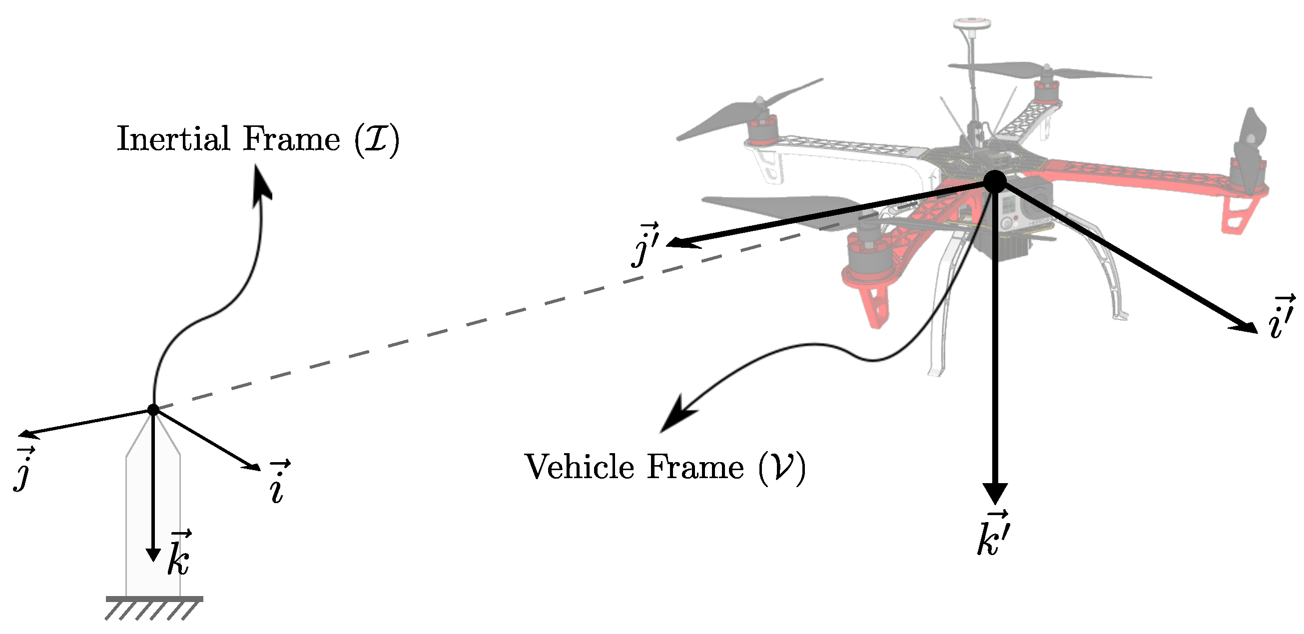
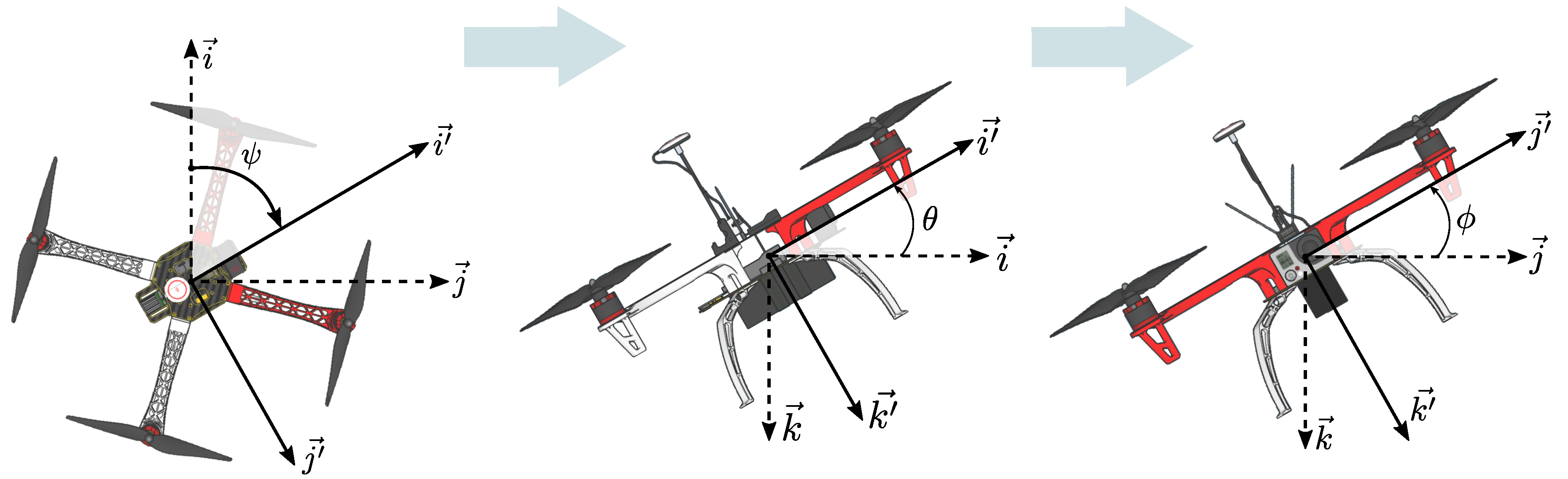
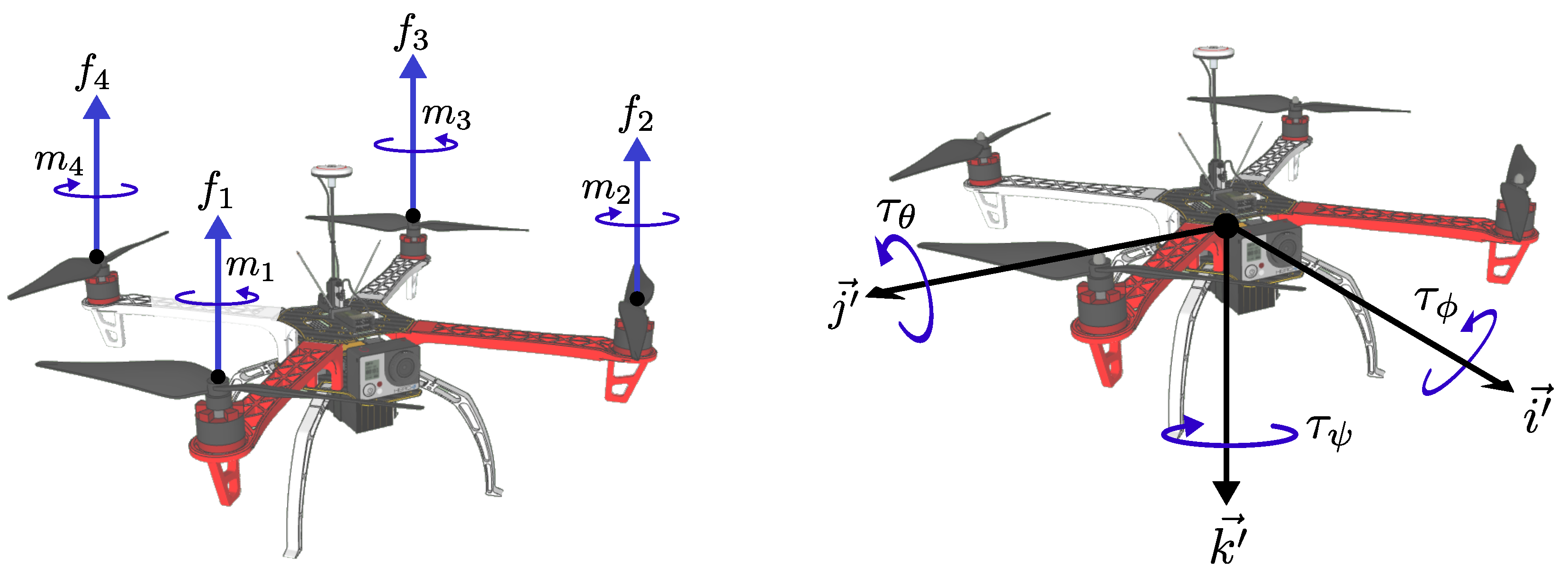
2.1. Mathematical Model of the Quadrotor

The quadrotor considered in this paper consists of a miniature UAV, which has the configuration of four coplanar rotors. The controlled variation of the rotors enables the movement of the quadrotor. The mathematical description of these movements begins with the assignment of the reference frames. This enables the measurement of changes in linear and angular position over time of the system.

The first reference frame is the inertial frame ($\mathcal{I}$). It is a fixed coordinate system whose axes point according to the NED system (north ($\overrightarrow{i}$), east ($\overrightarrow{j}$), down ($\overrightarrow{k}$)). The second is the vehicle frame ($\mathcal{V}$). It consists of a coordinate system in motion, located at the center of mass of the UAV. Its axes have the same direction as those of the $\mathcal{I}$ frame. Both reference frames are shown in Figure 1. The last reference frame is the body frame ($\mathcal{B}$), obtained by applying rotations on the $\mathcal{V}$ frame. These rotations determine the orientation of the UAV. They are carried out following a rotation order with the positive sense of the rule of the right hand: first on the axis $\overrightarrow{k}$, giving the yaw angle ($\psi$); then on the axis $\overrightarrow{j}$, giving the pitch angle ($\theta$); and finally on the axis $\overrightarrow{i}$, giving the roll angle ($\varphi$). This set of rotations generates the $\mathcal{B}$ frame, as shown in Figure 2.

The model that describes the quadrotor is nonlinear with 12 states [31] and three position states (X, Y, Z), aligned with $\overrightarrow{i}$, $\overrightarrow{j}$ and $\overrightarrow{k}$ axes of $\mathcal{I}$, three linear velocity states (U, V, W) in $\mathcal{B}$, three angular states ($\varphi$, $\theta$, $\psi$) and three angular velocity states (p, q, r) in $\mathcal{B}$. By using the Newton–Euler technique applied to this model, the full equations of the quadrotor dynamics are [32]:

$$\left[\begin{array}{c}\dot{X}\\ \dot{Y}\\ \dot{Z}\end{array}\right]=\left[\begin{array}{ccc}{c}_{\theta }{c}_{\psi }& s_{\varphi }{s}_{\theta }{c}_{\psi }-c_{\varphi }{s}_{\psi }& c_{\varphi }{s}_{\theta }{c}_{\psi }+s_{\varphi }{s}_{\psi }\\ c_{\theta }{s}_{\psi }& s_{\varphi }{s}_{\theta }{s}_{\psi }+c_{\varphi }{c}_{\psi }& c_{\varphi }{s}_{\theta }{s}_{\psi }-s_{\varphi }{c}_{\psi }\\ -s_{\theta }& s_{\varphi }{c}_{\theta }& c_{\varphi }{c}_{\theta }\end{array}\right]\left[\begin{array}{c}U\\ V\\ W\end{array}\right]$$

(1)

$$\left[\begin{array}{c}\dot{U}\\ \dot{V}\\ \dot{W}\end{array}\right]=\left[\begin{array}{c}rV-qW\\ pW-rU\\ qU-pV\end{array}\right]+\mathrm{g}\left[\begin{array}{c}-s_{\theta }\\ c_{\theta }{s}_{\varphi }\\ c_{\theta }{c}_{\varphi }\end{array}\right]+{\displaystyle \frac{1}{\mathrm{m}}}\left[\begin{array}{c}0\\ 0\\ {\tau }_z\end{array}\right]$$

(2)

$$\left[\begin{array}{c}\dot{\varphi }\\ \dot{\theta }\\ \dot{\psi }\end{array}\right]=\left[\begin{array}{ccc}1& s_{\varphi }{s}_{\theta }/c_{\theta }& -c_{\varphi }{s}_{\theta }/c_{\theta }\\ 0& c_{\varphi }& -s_{\varphi }\\ 0& s_{\varphi }/c_{\theta }& c_{\varphi }/c_{\theta }\end{array}\right]\left[\begin{array}{c}p\\ q\\ r\end{array}\right]$$

(3)

$$\left[\begin{array}{c}\dot{p}\\ \dot{q}\\ \dot{r}\end{array}\right]={\mathrm{J}}^{-1}\left(-\left[\begin{array}{c}p\\ q\\ r\end{array}\right]\times \mathrm{J}\left[\begin{array}{c}p\\ q\\ r\end{array}\right]+\left[\begin{array}{c}{\tau }_{\varphi }\\ {\tau }_{\theta }\\ {\tau }_{\psi }\end{array}\right]\right)$$

(4)

with $c_{\varphi }=\cos \left(\varphi \right)$, $c_{\theta }=\cos \left(\theta \right)$, $c_{\psi }=\cos \left(\psi \right)$, $s_{\varphi }=\sin \left(\varphi \right)$, $s_{\theta }=\sin \left(\theta \right)$ and $s_{\psi }=\sin \left(\psi \right)$. $\mathrm{g}$ is the gravity constant; $\mathrm{m}$ denotes the mass of the UAV; ${\tau }_z$ is the sum of the vertical forces generated by each propeller; $\tau ={[{\tau }_{\varphi },{\tau }_{\theta },{\tau }_{\psi }]}^T$ denotes the torque vector with its roll, pitch and yaw components; and the inertia matrix $\mathrm{J}$ is represented by:

$$\mathrm{J}=\left[\begin{array}{ccc}{\mathrm{J}}_X& 0& 0\\ 0& {\mathrm{J}}_Y& 0\\ 0& 0& {\mathrm{J}}_Z\end{array}\right].$$

(5)

Figure 3 shows the control input terms [${\tau }_z$, ${\tau }_{\varphi }$, ${\tau }_{\theta }$, ${\tau }_{\psi }$] which are generated by the composition of the forces $\left[f_1,f_2,f_3,f_4\right]$ and torques $\left[m_1,m_2,m_3,m_4\right]$ generated by the four rotors. d is the diameter of the UAV; i.e., the distance between the rotation axes of rotor 1 and rotor 2. This relationship is expressed as follows:

$$\begin{array}{ccc}\hfill {\tau }_z& =& \left(f_1+f_2+f_3+f_4\right),\hfill \end{array}$$

(6)

$$\begin{array}{ccc}\hfill {\tau }_{\varphi }& =& \frac{d}{\sqrt{2}}\left(-f_1+f_2+f_3-f_4\right),\hfill \end{array}$$

(7)

$$\begin{array}{ccc}\hfill {\tau }_{\theta }& =& \frac{d}{\sqrt{2}}\left(f_1+f_2-f_3-f_4\right),\hfill \end{array}$$

(8)

$$\begin{array}{ccc}\hfill {\tau }_{\psi }& =& \left(-m_1+m_2+m_3-m_4\right).\hfill \end{array}$$

(9)

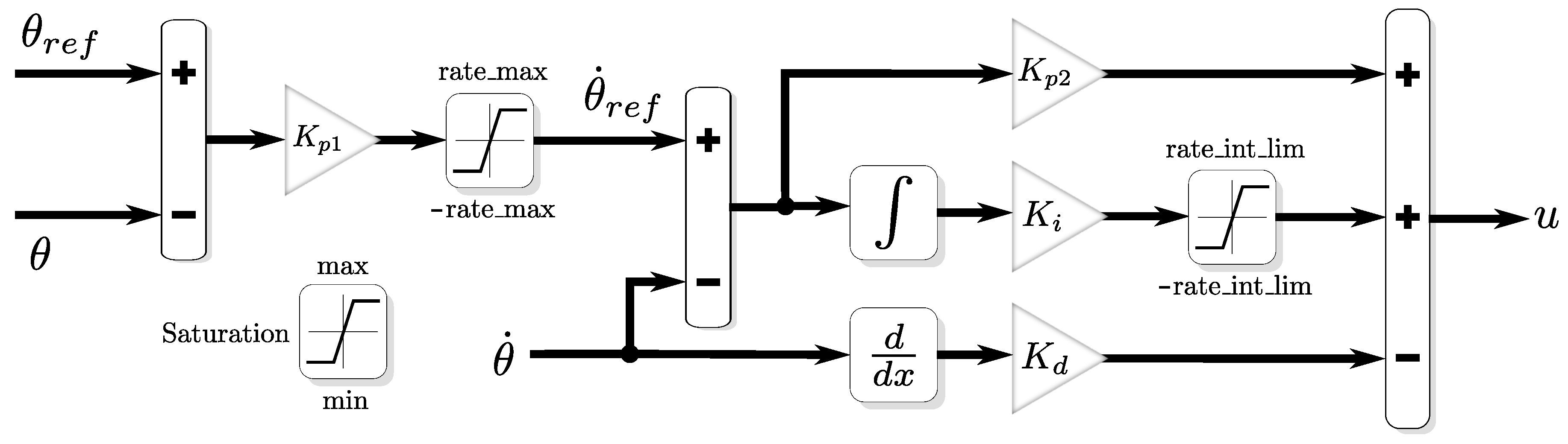
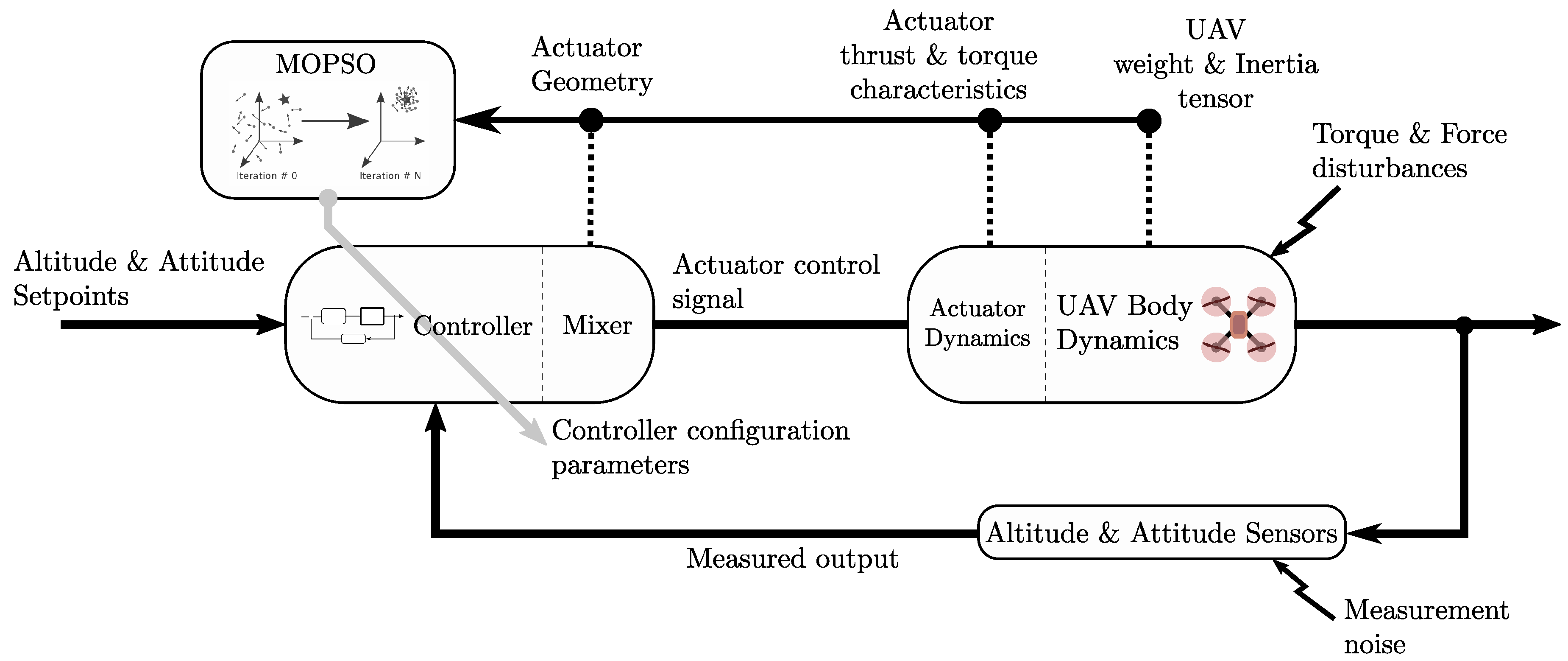
2.2. Control Architecture

PX4 uses PID controllers. That is the most widespread control technique [27]. The Px4-based UAV controllers are layered, which means an outer P-based attitude closed-loop controller passes its results to an inner PID-based velocity closed-loop controller, with feed-forward, as shown in Figure 4. The output of the proportional controller is limited to a defined range as well as the output of the integrative part of the PID controller. For this work, all ranges are set to their default values. The altitude control is analogous to the attitude one, although a constant "hovering thrust control" value is added to the output of this controller. That thrust control value is such that the UAV could fly without acceleration on the altitude axis when this controller has a zero output. Again, for this work, the hovering thrust control value is set to its default value. All controllers operate at the same time in parallel. In the system, the reference input consists of the Euler angles and altitude, and the rate of change of each of these variables. The Euler angles and angular rates are in radians and radians per second, respectively. The altitude and vertical speed are in meters and meters per second, respectively. The control efforts are the moments in each direction that, after being projected onto the body frame, are used to find the thrust of each motor-propeller assembly. Since there are four degrees of freedom (roll, pitch, yaw and vertical thrust), there are a total of 16 parameters to be optimized, which leads to four control actions $u_j$, with $j=1,2,3,4$, as shown in (10). Then, the gain values ${\left(K_{p1}\right)}_j$, ${\left(K_{p2}\right)}_j$, ${\left(K_i\right)}_j$ and ${\left(K_d\right)}_j$ are the control parameters to be optimized as in (10).

$$u_j={\left(K_{p2}\right)}_j{e}_j+{\left(K_i\right)}_j{\int }_0^t{e}_j\left(\tau \right)d\tau +{\left(K_d\right)}_j\frac{\mathrm{d}{e}_j}{\mathrm{d}t},j=1,2,3,4.$$

(10)

First, as it can be seen in Figure 4, the controller takes an attitude or altitude value $(\varphi ,\theta ,\psi ,Z)$ as the reference (setpoint) and compares it with the actual value obtained by the corresponding sensor. The difference between these two corresponds to the position error. This error is then multiplied by ${\left(K_{p1}\right)}_j$ and the result of this product is used as a reference for the rate of change of the corresponding degree of freedom. This new reference is then compared with the actual rate of change, again measured by the corresponding sensor, thereby obtaining the actual error $e_j$ used in (10). Figure 5 shows the overall control structure.

Remark 1.

The PID gain values are limited by default in the Px4 software to a range specified in [34] and shown in

Table 1. Allowable parameter ranges of the quadrotor UAV PID controller [34].

Axis	min ${\mathit{K}}_{\mathit{p}1}$	max ${\mathit{K}}_{\mathit{p}1}$	min ${\mathit{K}}_{\mathit{p}2}$	max ${\mathit{K}}_{\mathit{p}2}$	min ${\mathit{K}}_{\mathit{i}}$	max ${\mathit{K}}_{\mathit{i}}$	min ${\mathit{K}}_{\mathit{d}}$	max ${\mathit{K}}_{\mathit{d}}$
Roll	0	12	0	0.5	0	0.2	0	0.01
Pitch	0	12	0	0.6	0	0.2	0	0.01
Yaw	0	5	0	0.6	0	0.2	0	0.1
Altitude	0	1.5	0.1	0.4	0.01	0.1	0	0.1

. Note that the differential gain is much smaller because high values can cause the motors to overheat, because that part of the controller amplifies the noises [27].

Remark 2.

Note that the nominal quadrotor UAV model represented by (3)–(9) is used to compute the optimal PID gains offline. The gains so obtained are valid for small variations in the model parameters.

3. Proposed Tuning Procedure for the Gains of the PID Controller Based on MOPSO

This section presents the computation of the gains for the PID controller for the UAV. First, the basics of the PSO algorithm and its version for multiple-objective optimization, namely, the MOPSO algorithm, are presented. The proposed algorithm appears at the end of this section. The details of the Algorithm are given for better understanding and use by others.

3.1. Particle Swarm Optimization (PSO) Algorithm

The PSO algorithm is a stochastic, population-based algorithm first proposed in [35]. It was inspired by the collective behavior of animals, where it has been noticed that the behavior of each individual of a swarm can affect the behavior of the entire swarm and vice-versa by sharing useful information and using it together with personal experience to make decisions about how to act. These exchanges of information are beneficial to the search capability of the particles and offer a way of trading-off the speed of convergence and the time needed for the exploration. In the PSO algorithm, all of the particles in the swarm move in a space that is defined by all possible values that the decision variables can take. This space is known as the search-space. When a particle moves, the algorithm evaluates the parameters taken by the corresponding particle according to a fitness function $\mathbf{f}\left({\mathbf{x}}_n\right)$. Usually, the objective of the algorithm is to minimize $\mathbf{f}\left({\mathbf{x}}_n\right)$. Each particle ${\mathbf{x}}_n$ in the swarm of N particles has a velocity of ${\mathbf{v}}_n$, which determines its location in the search-space for the next iteration (t + 1) according to [36]:

$${\mathbf{x}}_n^{(t+1)}={\mathbf{x}}_n^{\left(t\right)}+\chi {\mathbf{v}}_n^{\left(t\right)}+{ϵ}^{\left(t\right)},$$

(11)

where $\chi$∈ [0,1] is a constraint value used to limit the velocity of each particle and $ϵ$ is a vector with random, uniformly-distributed components in the range [−1, 1]. This allows the algorithm to increase the range of exploration of the swarm to avoid local minima. The velocity ${\mathbf{v}}_n$ of the particles is modified so that these move towards the best position found so far by the particle. To summarize, the personal guide ${\mathbf{Pb}}_n$ (also called personal best), and the global guide Gb (global best; i.e., the best position found by the whole swarm) achieve an exchange of information between the particles. All of this is accomplished by updating the velocity vector by using the following equation:

$${\mathbf{v}}_n^{(t+1)}=w{\mathbf{v}}_n^{\left(t\right)}+r_1{c}_1({\mathbf{P}}_n-{\mathbf{x}}_n^{\left(t\right)})+r_2{c}_2(\mathbf{Gb}-{\mathbf{x}}_n^{\left(t\right)}),$$

(12)

where $r_1$ and $r_2$ are random evenly distributed numbers in the range of [0,1]; $c_1$ and $c_2$ are control factors that establish the influence of global and personal knowledge. Finally, w is a factor of inertia, which controls the trade-off between convergence and exploration.

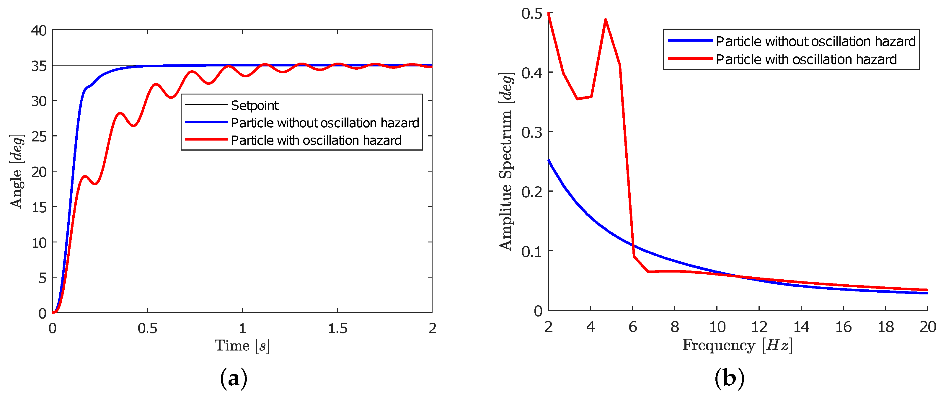
3.2. Multi-Objective Particle Swarm Optimization (MOPSO) Algorithm

Since the PSO is based on a simple concept, and is both fast and computationally inexpensive regarding memory requirements compared to other population techniques, it has been extended to handle multi-objective optimization problems. The majority of MOPSO algorithms share the same basic approach—a swarm of a certain number of agents is initialized randomly, and that number will remain constant until the end of the run. The swarm behavior is bounded by the velocity equation, which is updated continuously and is dependent on both the previous weighted velocity and known good solutions. In optimization problems with multiple objectives, a set of D objectives have to be optimized. These D objectives ($y_i$) depend on a vector x of K decision variables:

$$y_i=\mathbf{f}\left({\mathbf{x}}_n\right)\forall i=1,2,3,\cdots ,D,$$

(13)

According to the Pareto [30] optimal principle, a vector $\alpha$ strictly dominates another one $\beta$ (denoted $\alpha$≺$\beta$) if:

$${\mathbf{f}}_i\left(\alpha \right)<{\mathbf{f}}_i\left(\beta \right)\forall i=1,2,3,\cdots ,D,$$

(14)

and $\alpha$ weakly dominates $\beta$ (denoted $\alpha ⪯\beta$) if:

$${\mathbf{f}}_i\left(\alpha \right)\le {\mathbf{f}}_i\left(\beta \right)\forall i=1,2,3,\cdots ,D.$$

(15)

The Pareto front is the set of all non-dominated solutions while the Pareto optimal is a set of vectors that correspond to the Pareto front. In a multi-objective optimization problem, the target is usually to find a well-distributed Pareto front. In this paper, overshoot, rise time and root-mean-square error values of the step response values are considered as objectives for the optimization. All values are obtained by using the mathematical model of the quadrotor UAV. However, other performance parameters such as undershoot or settling time can be considered as well.

The main difficulty of using the PSO for multiple objective problems is how to choose the best guides. One approach that can be used is to make a single fitness function equal to a weighted sum of the objectives [28]. In this case, it is difficult to control the trade-off relationship between the different objectives. Moreover, there is a high probability of falling into local minima, making it difficult to obtain optimal values. As with other multiple objective algorithms, the concept of Pareto optimal is used as the fitness function, so that the user can choose a solution from the Pareto front. This approach has shown good results in previous works [30,31,32,33,34,35,36,37]. As a consequence, this method has been chosen in this paper.

For the implementation of the MOPSO, a repository A of non-dominated particles constitutes the optimal particles that correspond to the Pareto front. When a particle finds a new non-dominated position, the MOPSO algorithm checks if the particle dominates its previous personal guide or any element from A and removes them if that is the case, adding then the new particle to A. If the previous personal best is also not dominated, the new personal best is chosen randomly between the previous one and the new particle. The selection of the global guide for each particle A is based on "PROB" method described in [30] for selecting the best global guides. In PROB, for each particle ${\mathbf{x}}_n$, a global guide one is chosen between the particles of A that dominate ${\mathbf{x}}_n$. The guide is chosen randomly with a probability function proportional to the inverse of the number of particles of the swarm that are dominated currently by those particles. In the case that ${\mathbf{x}}_n$ belongs to A, a particle of A is chosen randomly with the same probability function as before. To keep the particles in the search space, the "SHR" method (proposed in [30]) is used. That is, assuming that the k-th component of a particle ${\mathbf{x}}_n$ exceeds its corresponding boundary B, the magnitude of ${\mathbf{v}}_n$ is shrunk according to:

$${\mathbf{x}}_n^{(t+1)}={\mathbf{x}}_n^{\left(t\right)}+\sigma (\chi {\mathbf{v}}_n^{\left(t\right)}+{ϵ}^{\left(t\right)}),$$

(16)

with

$$\sigma ={\displaystyle \frac{{\mathbf{x}}_{nk}^{\left(t\right)}-B}{\chi {\mathbf{v}}_{nk}^{\left(t\right)}+{ϵ}_k}},$$

(17)

so that the particle arrives exactly at the limit of the search-space.

3.3. Proposed Tuning Procedure

To evaluate the tuning performance of the algorithm, the UAV and its controller were simulated by using Equations (1)–(10). For the simulation, the script needs three inputs explained below:

• The mass $\mathrm{m}$ of the UAV. This can be computed by measuring it directly on a scale or by using an estimation method such as that proposed in [38].
• The moment of inertia $\mathrm{J}$ of the UAV. This input consists of the moment of inertia in the three-axes, $\left[J_X,J_Y,J_Z\right]$. These values can be obtained by using the pendulum method [39]. However, CAD Software such as Solidworks can be used to compute the moments of inertia as well.
• The torque and thrust responses of the propellers. A method to find these values is shown in Section 4.1. This method allows one to define a relationship between the responses and the pulse-width modulation (PWM) signals issued by the controller. However, an alternative could be to just use maximum thrust and torque that will be loaded.

Furthermore, the number of particles N, the number of generations G, the control factors $c_1$, $c_2$ and w, the velocity constraint value $\chi$ and the boundaries of the search space B have to be defined. Since the UAV is highly symmetrical, it is assumed that the moment of inertia tensor $\mathrm{J}$ is diagonal. This also allows the different attitude controllers to be decoupled, and therefore one can tune the different axis controllers independently by restricting the movement on the other axes. On each evaluation, the UAV starts at zero position and velocity in every degree of freedom and then the algorithm analyzes the step response of the UAV. The proposed tuning procedure based on MOPSO is run once for each axis to obtain its corresponding tuned parameters. The tuning procedure can be summarized by the pseudocode shown in Algorithm 1, where x is the set of all the particles whose number is defined beforehand, and v is the set of correspondent velocities of those particles.

Algorithm 1 Proposed tuning procedure based on the MOPSO algorithm.

$c_1,c_2,w,G,N,\chi \leftarrow define$ {Assign values to the control factors.} $\mathbf{x},\mathbf{v},{\mathbf{Pb}}_n,\mathbf{Gb}\leftarrow initialize\left(\right)$ {Randomly initialize particles and their velocities} $\mathbf{A}\leftarrow \varnothing$ {Initially empty archive} while $t\le G$ do  while $n\le N$ do   $ϵ\leftarrow random$ {Update the random vector.}   Update ${\mathbf{v}}_n^{\left(t\right)}$ with (12).   Update ${\mathbf{x}}_n^{\left(t\right)}$ with (11).   if ${\mathbf{x}}_n^{\left(t\right)}$ exceeds a boundary then    Enforce constraints with (16) and (17)   end if   $[K_{p1},K_{p2},K_i,K_d]\leftarrow {\mathbf{x}}_n^{\left(t\right)}$ {Use the position of the particle as the parameters for a new PID controller.}   Simulate UAV with its new controller’s gains.   ${\mathbf{y}}_n^{\left(t\right)}\leftarrow [O,RMSE,RT]$ {Overshoot (O), root-mean-square error (RMSE) and rise-time (RT) are used as objectives, these are obtained from the UAV simulation}   if $\gamma$ $⋠{\mathbf{x}}_n^{\left(t\right)}\forall$$\gamma$ $\in A$ then    $\mathbf{A}\leftarrow \gamma \in \mathbf{A}\mid {\mathbf{x}}_n^{\left(t\right)}\nprec \gamma$ {Remove particles dominated by ${\mathbf{x}}_n^{\left(t\right)}$ from A}    $\mathbf{A}\leftarrow \mathbf{A}\cup {\mathbf{x}}_n^{\left(t\right)}$ {Add ${\mathbf{x}}_n^{\left(t\right)}$ to A}   end if   if ${\mathbf{x}}_n^{\left(t\right)}⪯{\mathbf{Pb}}_n\vee ({\mathbf{x}}_n^{\left(t\right)}\nprec {\mathbf{Pb}}_n\wedge {\mathbf{Pb}}_n\nprec {\mathbf{x}}_n^{\left(t\right)})$ then    ${\mathbf{Pb}}_n\leftarrow {\mathbf{x}}_n^{\left(t\right)}$ {Update personal guide}   end if   $\mathbf{Gb}\leftarrow {\mathbf{A}}_j$ {Update global guide for the next particle. Here, j is an index from A chosen randomly using PROB (see Section 3.2).}   $n:=n+1$  end while  $t:=t+1$ end while Select one of the particles from A as the final tuning.

4. Simulation and Experimental Results

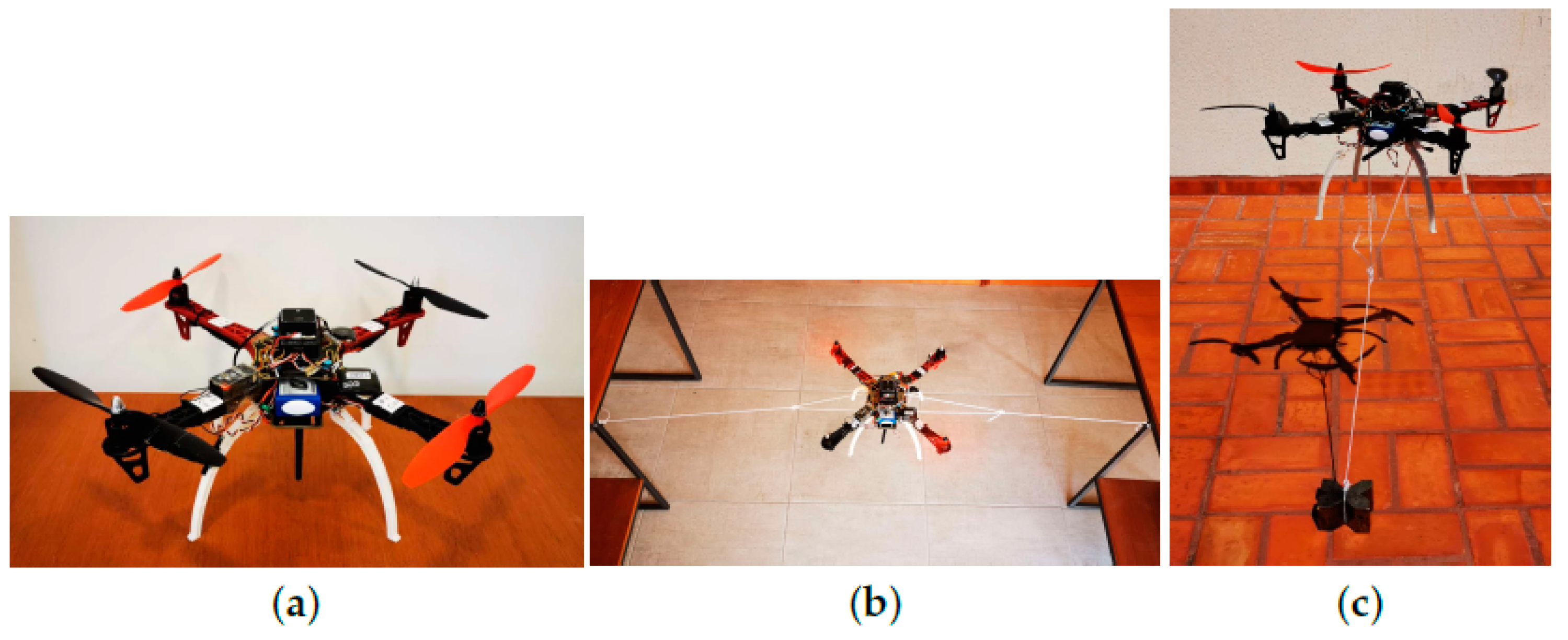
4.1. Quadrotor Parameters

In this section, simulation and experimental results are provided to evaluate the performance of the proposed PID controller design procedure under several gains obtained by MOPSO. In all tests, the quadrotor parameters shown in

Table 2. Quadrotor UAV parameters.

Parameter	Value
a = b	$0.1700$ m	(X, Y, Z axes)
h	$0.2360$ m	(X axis)
h	$0.2660$ m	(Y axis)
h	$0.4350$ m	(Z axis)
$\mathrm{g}$	$9.81$ m/s${}^2$
$\mathrm{m}$	$1.3240$ kg

were used. A photo of the actual quadrotor used for validation is shown in Figure 6a. Figure 6b,c show the same quadrotor with the test base, which is explained later in Section 4.2.1. Other inputs needed for the computation of the PID gains using the MOPSO algorithm, such as the moments of inertia, torque and thrust responses of the propellers, are introduced next.

The moment of inertia $\left[J_X,J_Y,J_Z\right]$ of a UAV from its center of gravity with respect to its axes of rotation can be computed by using Equation (18). This is the bifilar pendulum method [39]. Therefore, the geometric values a, b, h, $\mathrm{m}$ are needed. The measured oscillation frequency $\mathrm{f}$ is also needed. The values so obtained are given in

Table 3. Computed moment of inertia of the quadrotor.

Moment of Inertia	Value
$J_X$	$0.0124$ kgm${}^2$
$J_Y$	$0.0130$ kgm${}^2$
$J_Z$	$0.0237$ kgm${}^2$

.

$$J_i={\displaystyle \frac{\mathrm{m}\mathrm{g}ab}{h{\left(2\pi \mathrm{f}\right)}^2}},i=X,Y,Z.$$

(18)

The relatively simple functions, represented by Equations (19) and (20), are then used to determine the thrust and torque produced by each motor based on the value of the duty cycle of the PWM signal of each motor. These functions have a polynomial form, where $f_i$ and $m_i$ represent the nth order polynomial functions of the thrust (in N) and the torque (in Nm), respectively with respect to the $X_{PWM}$∈ [1000, 2000]. In this work, n = 5 was used.

$$f_i=\sum _{k=0}^{k=n}{X}_{PWM}^k{P}_{thrust}^k,$$

(19)

$$m_i=\sum _{k=0}^{k=n}{X}_{PWM}^k{P}_{torque}^k.$$

(20)

These functions were obtained through a series of tests of each motor in which several points were obtained, after which a polynomial approximation was made to obtain the coefficients $P_{thrust}^k$ and $P_{torque}^k$. After obtaining these averages, a polynomial regression was performed with the order n specified above, obtaining the coefficients of the polynomials that define the functions $f_i$ and $m_i$ respectively. The polynomials so obtained were:

$$\begin{array}{ccc}\hfill P_{thrust}& =& [-{2.315}^{-14},{1.680}^{-10},-{4.860}^{-7},0.001,-0.505,143],\hfill \end{array}$$

(21)

$$\begin{array}{ccc}\hfill P_{torque}& =& [-{3.323}^{-16},{2.417}^{-12},-{7.014}^{-9},{1.02}^{-5},-0.007,2.075].\hfill \end{array}$$

(22)

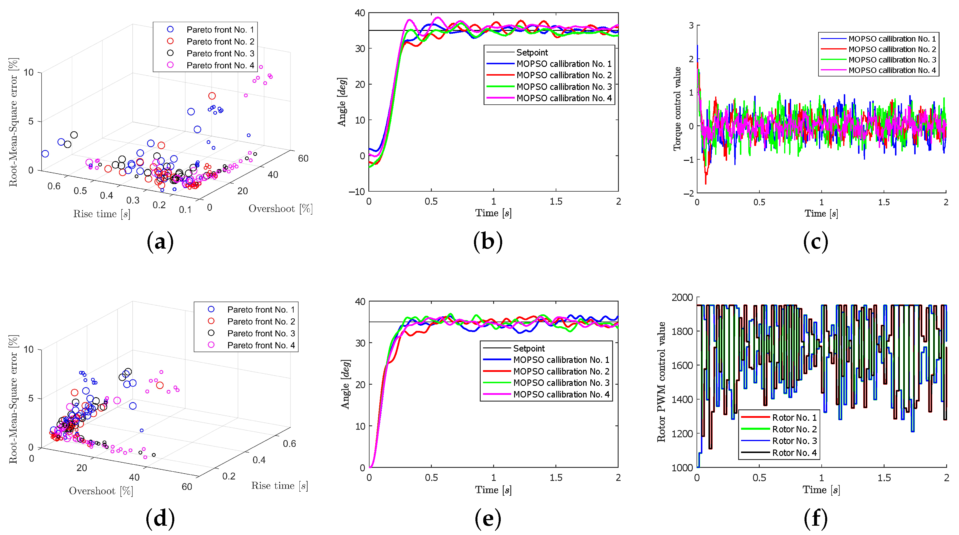
4.2. Simulation and Experimental Validation the Proposed MOPSO Algorithm

The proposed MOPSO algorithm was implemented in custom Matlab script. For this paper, the values $N=12$, $G=15$, $w=0.6$, $c_1=1$, $c_2=1$ and $\chi =1$ were empirically chosen. Then, by running the Matlab script with the known inputs explained in Section 3.3, the MOPSO algorithm searches for the Pareto optimal control parameters for both the attitude and the altitude controllers. The search for the parameters has been carried out for each PID controller sequentially in this order: (1) roll, (2) pitch, (3) yaw and (4) altitude axis. The values so obtained were then manually uploaded to the UAV through programs such as QgroundControl and MissionPlanner.

Since this work used the nominal model for the UAV quadrotor, the PID performance was evaluated by the obtained gains from the MOPSO algorithm under three scenarios. These scenarios give a true evaluation of the performance of the PID controller under variation of the parameters and/or the model of the system.

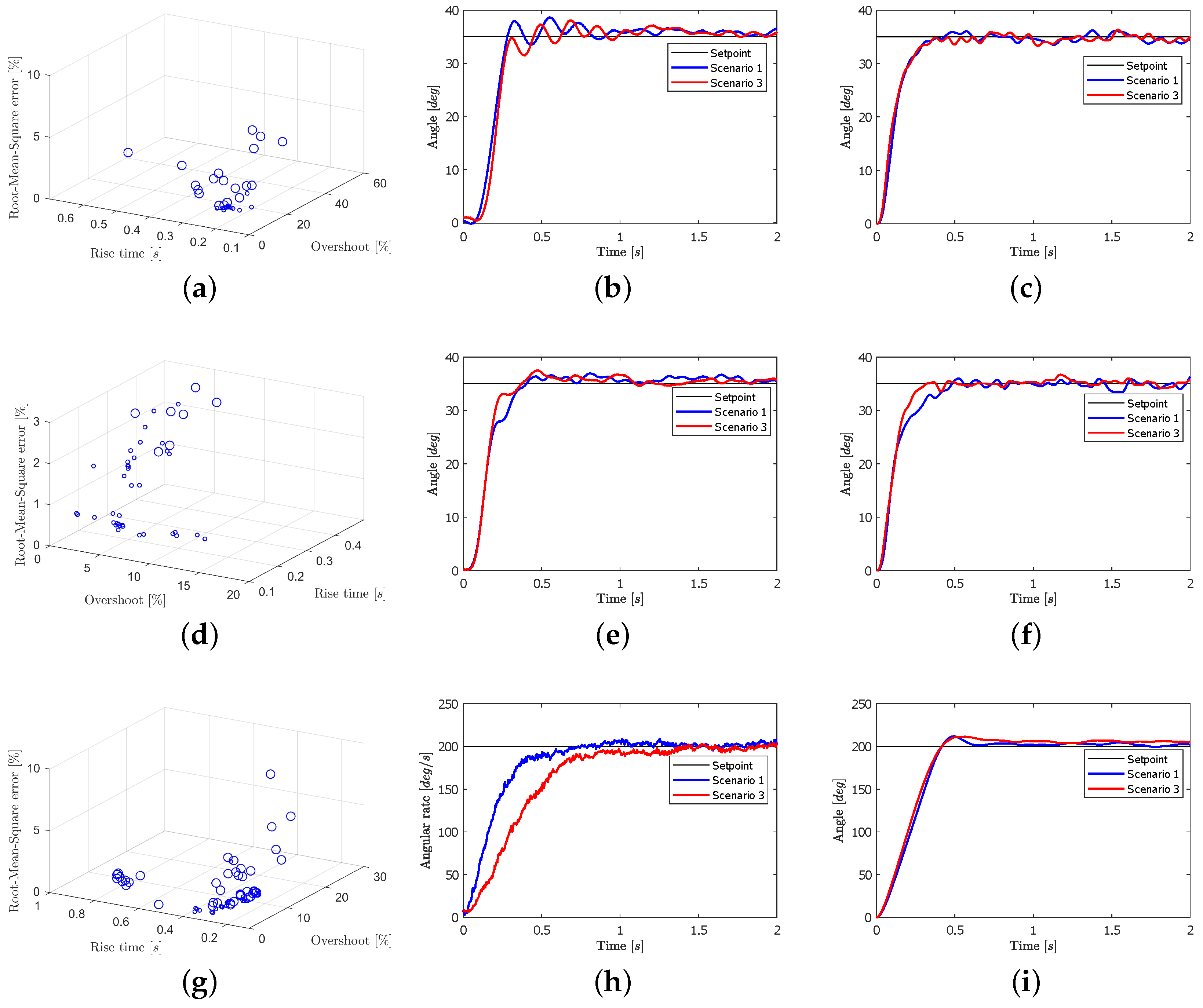
• Scenario 1: The model uses the nominal UAV parameters.
• Scenario 2: The UAV mass and inertia matrix values are changed by +15% relative to their nominal values. Moreover, the values of the diameter of the UAV, the $P_{thrust}$ and the $P_{torque}$ are also modified by −15% from their nominal values.
• Scenario 3: The UAV mass and inertia matrix values are changed by −15% relative to their nominal values. Moreover, the values of the diameter of the UAV, the $P_{thrust}$ and the $P_{torque}$ are also modified by +15% from their nominal values.

In order to make the MOPSO algorithm even more robust, a fourth dimension was added to the Pareto front and a dual evaluation was made for each particle. This fourth dimension was named "oscillation hazard." For the first evaluation process, in the case of the attitude controller calibration, the noise was added as the sum on the input port of the angle port with a value range of $-0.01$ to $0.01$ rad and on the input port of the angular rate with a value range of $-0.105$ to $0.105$ rad/s. In the case of the altitude controller calibration, the noise was added as the sum on the input port of the altitude port with a value range of $-0.091$ to $-0.09$ m and on the input port of the vertical speed with a value range of $-0.15$ to $0.1$ m/s. In this evaluation, the overshoot, rise time and root-mean-square error values were computed. For the second evaluation process, no noise was added to the input ports. In this evaluation, the oscillation hazard was computed. A fast Fourier transform (FFT) was evaluated on the step response covering the time that the axis value reached 96% of the value of the setpoint or until the end of the simulation. If the values of the FFT of the response have a gradient less than zero in the range of 2 Hz to 15 Hz, the oscillation hazard will have a value of "zero." In the other case, the oscillation hazard value will be set to "one." A value of "zero" for the oscillation hazard ensures that the evaluated particle will not cause the real UAV to oscillate excessively. An example of this evaluation is shown in Figure 7.

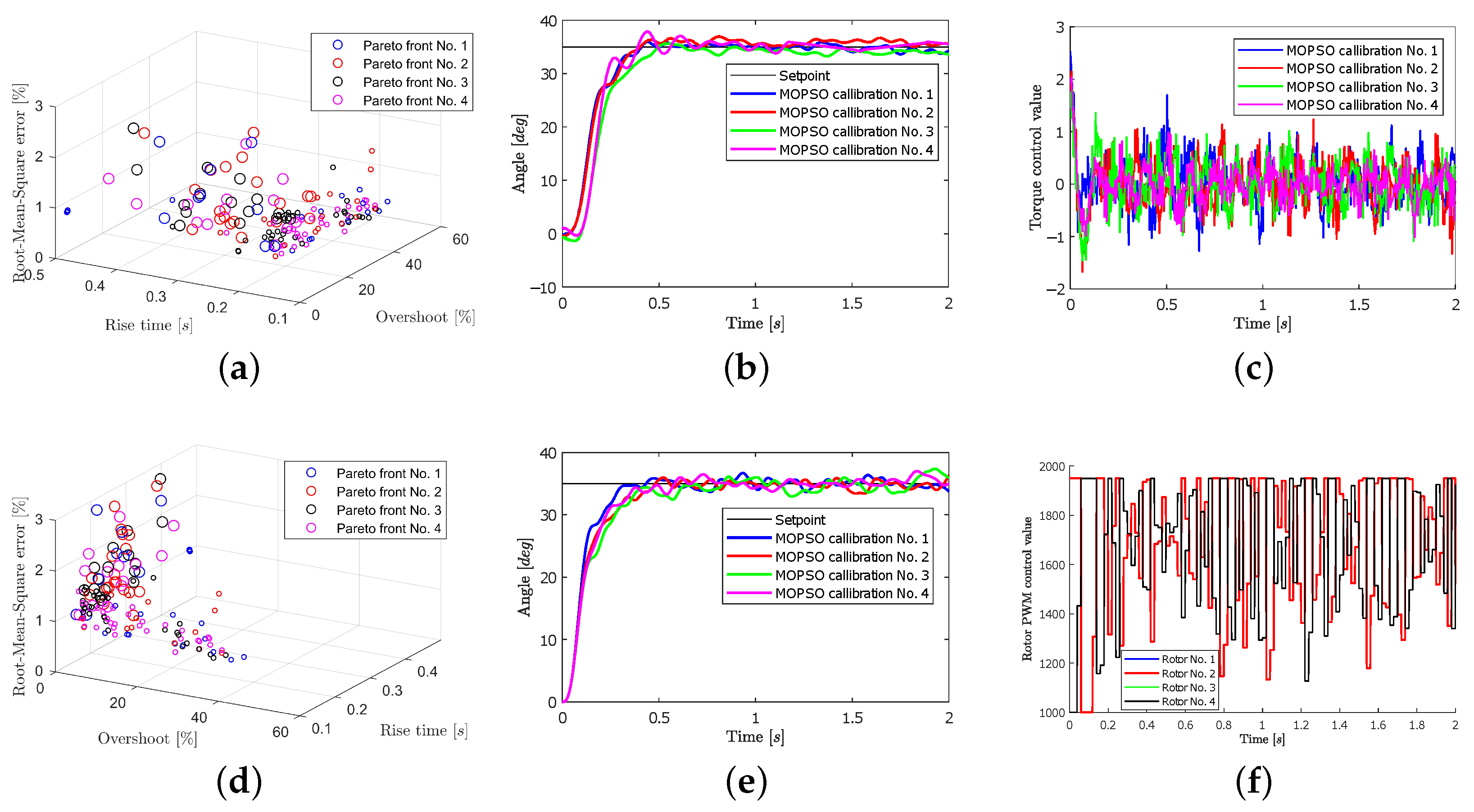
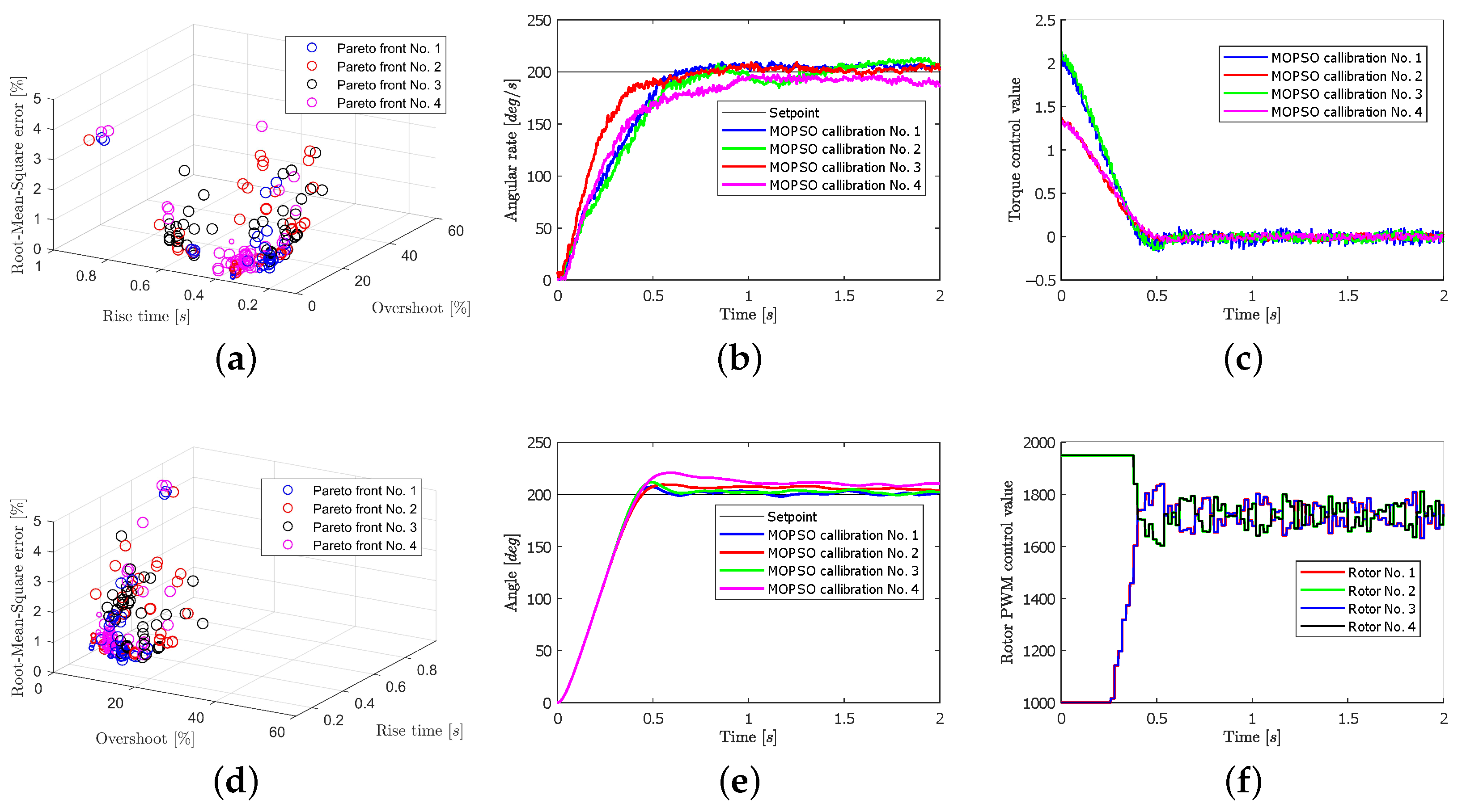
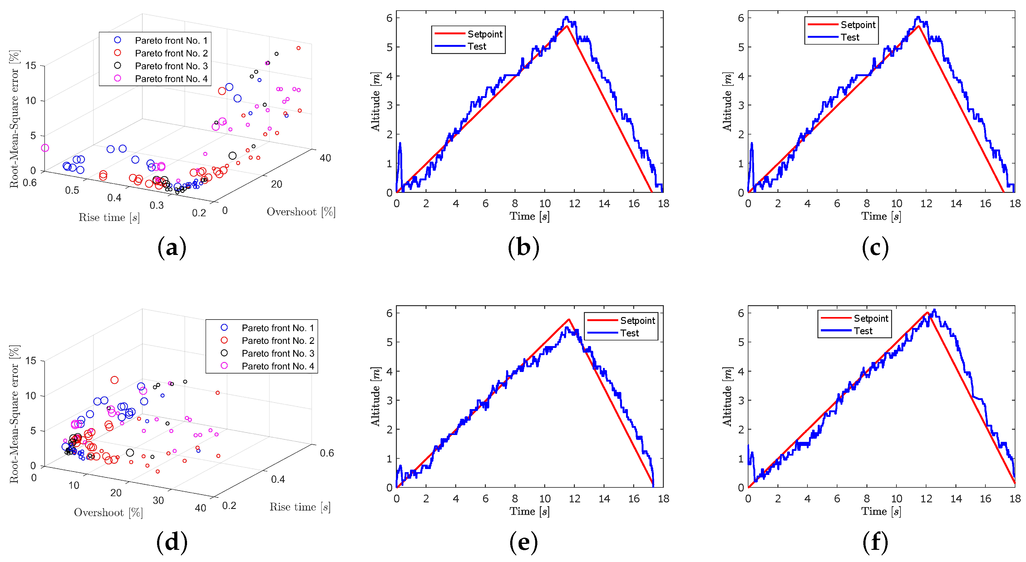
4.2.1. Scenario 1 Analysis

When the Algorithm 1 ends, the Pareto front of the optimal calibration parameters is formed. Any of the particles in the Pareto front are considered optimal, but criteria have to be established to select a particle from the Pareto front to be implemented in the PID controller. For this work, the particle with the least root-mean-square error and with an oscillation hazard value of zero was selected as the output of the MOPSO control calibration for each axis control. Then, from the Pareto front shown in Figure 8a and Figure 8d (roll axis); Figure 9a and Figure 9d (pitch axis); Figure 10a and Figure 10d (yaw axis); and Figure 11a and Figure 11d (altitude axis) the gains which matched the criteria for each axis were selected and tested by simulation and experimentation.

Table 4. Obtained control performance based on experimental results.

Axis	${\mathit{K}}_{\mathit{p}1}$	${\mathit{K}}_{\mathit{p}2}$	${\mathit{K}}_{\mathit{i}}$	${\mathit{K}}_{\mathit{d}}$	Overshoot	Rise Time	Root-Mean-Square Error
Roll	$9.5611$	$0.3727$	$0.1812$	$0.0064$	$10.5163$ %	$0.1448$ s	$2.0341$ %
Pitch	$7.4758$	$0.5640$	$0.0292$	$0.0100$	$5.7190$ %	$0.2248$ s	$1.7792$ %
Yaw	$3.4548$	$0.3840$	$0.0001$	$0.0001$	$4.62680$ %	$0.3176$ s	$1.6963$ %
Altitude	$1.2191$	$0.1895$	$0.0989$	$0.0001$	$--$	$--$	$0.3397$ m

shows gains so obtained for each axis as well as the performance parameters. The overshoot, rise time and root-mean-square error were computed from the logged angle response (for roll and pitch axes) and the logged rate response (for yaw axis).

The roll and pitch PID controllers were tested using the manual flight mode [40]. For security issues, the UAV was tied with ropes on a custom test base during the test. A constant setpoint value of 35 degrees was set remotely for the UAV in both axes and a step response was tested, as shown in Figure 8b and Figure 8d (roll axis) and Figure 9b and Figure 9d (pitch axis). It can be noted that there is a good agreement between the simulation and experimental results. Torque control actions and the generated PWM signals were also analyzed as shown in Figure 8c and Figure 8e (roll axis) and in Figure 9c and Figure 9e (pitch axis).

For the test of the yaw PID controller, the UAV was tied on an another custom test base shown in Figure 6c. For the test of the altitude PID controller, the UAV was set to fly freely (without a test base). For both tests, the altitude flight mode [41] was used. This flight mode allows the user to control the yaw rate and the vertical speed. The mission mode [42] allows the user to pre-define a flight plan that can control the altitude and the yaw angle. However, for this project it can not be used due to this mode requiring 3-D positional information from a global positioning system (GPS). For the yaw controller, a constant rate setpoint of 200 degrees/s was set remotely for the UAV, as shown in Figure 10b,e. Torque control actions and the generated PWM signals were plotted in Figure 10c,e for the yaw axis. For the altitude controller, a vertical rate setpoint of $0.5$ m/s upwards was set, and then it was changed to 1 m/s downwards until the UAV was landed. Four tests were performed as depicted in Figure 11b,c,e,f. Note that the altitude controller uses a barometric sensor for altitude measuring [41]. This type of sensor may become inaccurate in some conditions. As a consequence, the logged altitude data might be unreliable for providing accurate vertical speed data. For this work, the vertical setpoint values were integrated to obtain a time-variable altitude setpoint, and the mean-square error of the altitude along this setpoint was measured.

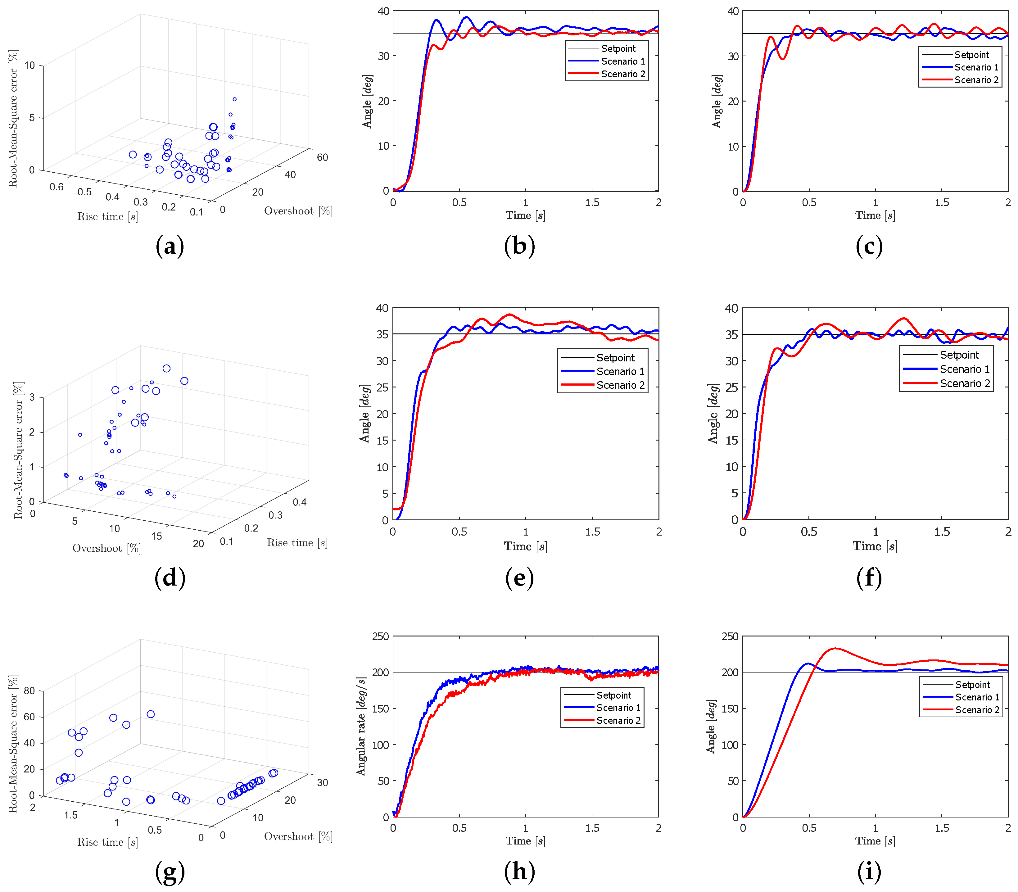
4.2.2. Scenario 2 Analysis

In this scenario, the PID controller was tested under parameter mismatch, as explained at the beginning of Section 4.2.1. Therefore, the tuning process with the MOPSO has performed appearing errors in the UAV model. Evaluations of the behavior of the PID controllers have been carried out and the results so obtained shown to be satisfactory, as shown in Figure 12 and Figure 13.

4.2.3. Scenario 3 Analysis

Analogously to the previous scenario, a modification of the parameters of the UAV was carried out as explained in Section 4.2.1. Again, the results so obtained demonstrate the correct operation of the PID controllers, as shown in Figure 14 and Figure 15. Thus, the proposed tuning method demonstrated itself to be robust against parameter mismatching and/or for the use of a simplified UAV model.

5. Conclusions

In this paper, an offline method for tuning the PID controller for a quadrotor, based on the MOPSO algorithm, has been introduced. The proposed method uses Pareto optimally for its fitness function so that the user can choose a desirable solution from the Pareto front, thereby ensuring that the solutions are aligned with the purposes of the user. The obtained gain values have been analyzed experimentally in the PID control structure that comes as the default in the firmware of the Px4-based quadrotor UAV. The results show good performance considering the optimization of the overshoot, rise time and root-mean-square error of step response of the PID. Additionally, the results were shown by the simulation to be robust against parameter changes. Note that the proposed method can be easily extended to other multirotor configurations (hexacopter, octocopter, etc.).

References

1. Prisacariu, V. The history and the evolution of UAVs from the beginning till the 70s. J. Def. Resour. Manag. (JoDRM) 2017, 8, 181–189. [Google Scholar]
2. Black, J. Air Power: A Global History; Rowman & Littlefield: Lanham, MD, USA, 2016; pp. 26–28. [Google Scholar]
3. Newcome, L.R. Unmanned Aviation: A Brief History of Unmanned Aerial Vehicles; American Institute of Aeronautics and Astronautics: Reston, VA, USA, 2004. [Google Scholar]
4. Marshall, D.M.; Barnhart, R.K.; Hottman, S.B.; Shappee, E.; Most, M.T. Introduction to Unmanned Aircraft Systems; CRC Press: Boca Raton, FL, USA, 2016; pp. 6–7. [Google Scholar]
5. Custers, B. Future of Drone Use; Springer: New York, NY, USA, 2016; p. 9. [Google Scholar]
6. Hundley, R.O.; Gritton, E.C. Future technology-driven revolutions in military operations; RAND Corporation: Santa Monica, CA, USA, 1994; Document No. DB-110-ARPA. [Google Scholar]
7. Miller, M. The Internet of Things: How Smart TVs, Smart Cars, Smart Homes, and Smart Cities are Changing the World; Pearson Education: London, UK, 2015. [Google Scholar]
8. Watts, A.C.; Ambrosia, V.G.; Hinkley, E.A. Unmanned aircraft systems in remote sensing and scientific research: Classification and considerations of use. Remote Sens. 2012, 4, 1671–1692. [Google Scholar] [CrossRef] [Green Version]
9. Brooke-Holland, L. Unmanned Aerial Vehicles (Drones): An Introduction; House of Commons Library: London, UK, 2012. [Google Scholar]
10. Arjomandi, M.; Agostino, S.; Mammone, M.; Nelson, M.; Zhou, T. Classification of Unmanned Aerial Vehicles; Report for Mechanical Engineering Class; University of Adelaide: Adelaide, Australia, 2006. [Google Scholar]
11. Weibel, R.E. Safety Considerations for Operation of Different Classes of Unmanned Aerial Vehicles in the National Airspace System. Ph.D. Thesis, Massachusetts Institute of Technology, Cambridge, MA, USA, 2005. [Google Scholar]
12. Kim, J.; Kim, S.; Ju, C.; Son, H.I. Unmanned aerial vehicles in agriculture: A review of perspective of platform, control, and applications. IEEE Access 2019, 7, 105100–105115. [Google Scholar] [CrossRef]
13. Kim, J.; Gadsden, S.A.; Wilkerson, S.A. A Comprehensive Survey of Control Strategies for Autonomous Quadrotors. Can. J. Electr. Comput. Eng. 2019, 43, 3–16. [Google Scholar]
14. Salih, A.L.; Moghavvemi, M.; Mohamed, H.A.; Gaeid, K.S. Modelling and PID controller design for a quadrotor unmanned air vehicle. In Proceedings of the 2010 IEEE International Conference on Automation, Quality and Testing, Robotics (AQTR), Cluj-Napoca, Romania, 28–30 May 2010; IEEE: Piscataway, NJ, USA, 2010; Volume 1, pp. 1–5. [Google Scholar]
15. Reyes-Valeria, E.; Enriquez-Caldera, R.; Camacho-Lara, S.; Guichard, J. LQR control for a quadrotor using unit quaternions: Modeling and simulation. In Proceedings of the CONIELECOMP 2013, 23rd International Conference on Electronics, Communications and Computing, Cholula, Puebla, Mexico, 11–13 March 2013; IEEE: Piscataway, NJ, USA, 2013; pp. 172–178. [Google Scholar]
16. Masuda, K.; Uchiyama, K. Robust control design for quad tilt-wing UAV. Aerospace 2018, 5, 17. [Google Scholar] [CrossRef] [Green Version]
17. Ataka, A.; Tnunay, H.; Inovan, R.; Abdurrohman, M.; Preastianto, H.; Cahyadi, A.I.; Yamamoto, Y. Controllability and observability analysis of the gain scheduling based linearization for uav quadrotor. In Proceedings of the 2013 International Conference on Robotics, Biomimetics, Intelligent Computational Systems, Yogyakarta, Indonesia, 25–27 November 2013; IEEE: Piscataway, NJ, USA, 2013; pp. 212–218. [Google Scholar]
18. Voos, H. Nonlinear control of a quadrotor micro-UAV using feedback-linearization. In Proceedings of the 2009 IEEE International Conference on Mechatronics, Málaga, Spain, 14–17 April 2009; IEEE: Piscataway, NJ, USA, 2009; pp. 1–6. [Google Scholar]
19. Lee, D.; Ha, C.; Zuo, Z. Backstepping control of quadrotor-type UAVs and its application to teleoperation over the internet. In Intelligent Autonomous Systems 12; Springer: New York, NY, USA, 2013; pp. 217–225. [Google Scholar]
20. Paiva, E.; Gomez-Redondo, M.; Rodas, J.; Kali, Y.; Saad, M.; Gregor, R.; Fretes, H. Cascade First and Second Order Sliding Mode Controller of a QuadRotor UAV based on Exponential Reaching Law and Modified Super-Twisting Algorithm. In Proceedings of the 2019 Workshop on Research, Education and Development of Unmanned Aerial Systems (RED UAS), Cranfield, UK, 25–27 November 2019; IEEE: Piscataway, NJ, USA, 2019; pp. 100–105. [Google Scholar]
21. Kali, Y.; Rodas, J.; Saad, M.; Gregor, R.; Alqaisi, W.; Benjelloun, K. Robust Finite-time Position and Attitude Tracking of a Quadrotor UAV using Super-Twisting Control Algorithm with Linear Correction Terms. In Proceedings of the 16th International Conference on Informatics in Control, Automation and Robotics—Volume 2: ICINCO, Prague, Czech Republic, 29–31 July 2019; INSTICC, SciTePress: Setubal, Portugal, 2019; pp. 221–228. [Google Scholar] [CrossRef]
22. Paiva, E.; Rodas, J.; Kali, Y.; Gregor, R.; Saad, M. Robust flight control of a tri-rotor UAV based on modified super-twisting algorithm. In Proceedings of the 2019 International Conference on Unmanned Aircraft Systems (ICUAS), Atlanta, GA, USA, 11–14 June 2019; IEEE: Piscataway, NJ, USA, 2019; pp. 551–556. [Google Scholar]
23. Kang, Y.; Hedrick, J.K. Linear Tracking for a Fixed-Wing UAV Using Nonlinear Model Predictive Control. IEEE Trans. Control. Syst. Technol. 2009, 17, 1202–1210. [Google Scholar] [CrossRef]
24. Nafia, N.; El Kari, A.; Ayad, H.; Mjahed, M. Robust full tracking control design of disturbed quadrotor UAVs with unknown dynamics. Aerospace 2018, 5, 115. [Google Scholar] [CrossRef] [Green Version]
25. Dierks, T.; Jagannathan, S. Output feedback control of a quadrotor UAV using neural networks. IEEE Trans. Neural Netw. 2009, 21, 50–66. [Google Scholar] [CrossRef]
26. Liu, L.; Liang, X.; Zhu, C.; He, L. Distributed cooperative control for UAV swarm formation reconfiguration based on consensus theory. In Proceedings of the 2017 2nd International Conference on Robotics and Automation Engineering (ICRAE), Shanghai, China, 29–31 December 2017; IEEE: Piscataway, NJ, USA, 2017; pp. 264–268. [Google Scholar]
27. Px4 Tuning Guide. Available online: https://docs.px4.io/v1.9.0/en/config_mc/pid_tuning_guide_multicopter.html (accessed on 16 April 2020).
28. Mac, T.T.; Copot, C.; Duc, T.T.; De Keyser, R. AR.Drone UAV control parameters tuning based on particle swarm optimization algorithm. In Proceedings of the 2016 IEEE International Conference on Automation, Quality and Testing, Robotics (AQTR), Cluj-Napoca, Romania, 19–21 May 2016; IEEE: Piscataway, NJ, USA, 2016. [Google Scholar]
29. Jaafar, H.I.; Mohd Ali, N.; Mohamed, Z.; Selamat, N.; Zainal Abidin, A.F.; Jamian, J.J.; Kassim, A. Optimal Performance of a Nonlinear Gantry Crane System via Priority-based Fitness Scheme in Binary PSO Algorithm. IOP Conf. Ser. Mater. Sci. Eng. 2013, 53, 1–6. [Google Scholar] [CrossRef] [Green Version]
30. Alvarez-Benitez, J.E.; Everson, R.M.; Fieldsend, J.E. A MOPSO algorithm based exclusively on pareto dominance concepts. In Proceedings of the International Conference on Evolutionary Multi-Criterion Optimization, Guanajuato, Mexico, 9–11 March 2005; Springer: New York, NY, USA, 2005; pp. 459–473. [Google Scholar]
31. Beard, R.W.; McLain, T.W. Small Unmanned Aircraft: Theory and Practice; Princeton University Press: Princeton, NJ, USA, 2012. [Google Scholar]
32. Musa, S. Techniques for quadcopter modeling and design: A review. J. Unmanned Syst. Technol. 2018, 5, 66–75. [Google Scholar]
33. Ortiz, N.A.S.; Laroche, E.; Kiefer, R.; Durand, S. Controller tuning strategy for quadrotor MAV carrying a cable-suspended load. In Proceedings of the International Micro Air Vehicle Conference and Flight Competition (IMAV), Beijing, China, 17–21 October 2016. [Google Scholar]
34. Px4 Parameter Reference. Available online: https://docs.px4.io/v1.9.0/en/advanced_config/parameter_reference.html (accessed on 16 April 2020).
35. Kennedy, J.; Eberhart, R. Particle swarm optimization. In Proceedings of the ICNN’95-International Conference on Neural Networks, Perth, Australia, 27 November–1 December 1995; IEEE: Piscataway, NJ, USA, 1995; Volume 4, pp. 1942–1948. [Google Scholar]
36. Azabi, Y.; Savvaris, A.; Kipouros, T. The Interactive Design Approach for Aerodynamic Shape Design Optimisation of the Aegis UAV. Aerospace 2019, 6, 42. [Google Scholar] [CrossRef] [Green Version]
37. Coello, C.C.; Lechuga, M.S. MOPSO: A proposal for multiple objective particle swarm optimization. In Proceedings of the 2002 Congress on Evolutionary Computation, CEC’02 (Cat. No. 02TH8600), Chiang Mai, Thailand, 26–30 July 2002; IEEE: Piscataway, NJ, USA, 2002; Volume 2, pp. 1051–1056. [Google Scholar]
38. Ho, D.; Linder, J.; Hendeby, G.; Enqvist, M. Mass estimation of a quadcopter using IMU data. In Proceedings of the 2017 International Conference on Unmanned Aircraft Systems (ICUAS), Miami, FL, USA, 13–16 June 2017; IEEE: Piscataway, NJ, USA, 2017; pp. 1260–1266. [Google Scholar]
39. Krznar, M.; Kotarski, D.; Piljek, P.; Pavković, D. On-line Inertia Measurement of Unmanned Aerial Vehicles using on board Sensors and Bifilar Pendulum. Interdiscip. Descr. Complex Syst. INDECS 2018, 16, 149–161. [Google Scholar] [CrossRef] [Green Version]
40. Px4 Manual Mode. Available online: https://docs.px4.io/v1.9.0/en/flight_modes/manual_stabilized_mc.html (accessed on 16 April 2020).
41. Px4 Altitude Mode. Available online: https://docs.px4.io/v1.9.0/en/flight_modes/altitude_mc.html (accessed on 16 April 2020).
42. Px4 Mission Mode. Available online: https://docs.px4.io/v1.9.0/en/flight_modes/mission.html (accessed on 16 April 2020).
Figure 1. Configuration of a quadrotor considering the inertial frame ( I ) and the vehicle frame ( V ).
Aerospace 07 00071 g001
Figure 2. Quadrotor orientation, yaw ( ψ ), pitch ( θ ) and roll ( ϕ ) angles.
Aerospace 07 00071 g002
Figure 3. Quadrotor orientation, yaw ( ψ ), pitch ( θ ) and roll ( ϕ ) angles.
Aerospace 07 00071 g003
Figure 4. Position and attitude controller structure of a Px4-based UAV [33].
Aerospace 07 00071 g004
Figure 5. Altitude and attitude control of a Px4-based UAV with optimal PID computed offline by the proposed MOPSO algorithm.
Aerospace 07 00071 g005
Figure 6. (a) Quadrotor used for test the optimal gains for the PID controller. (b) Quadrotor with the test base for the roll and pitch axes controller test. (c) Quadrotor with the test base for the yaw axis controller test.
Aerospace 07 00071 g006
Figure 7. (a) Roll axis step response simulation for oscillation hazard determination. (b) FFT of roll axis step response simulation.
Aerospace 07 00071 g007
Figure 8. Results obtained for the roll axis. (a) Pareto front (the bigger particles represent the ones without oscillation hazard). (b) Experimental step response. (c) Torque control values. (d) Pareto front in a different perspective. (e) Simulation step response. (f) Pulse-width modulation (PWM) control value (calibration number 1).
Aerospace 07 00071 g008
Figure 9. Results obtained for the pitch axis. (a) Pareto front (the bigger particles represent the ones without oscillation hazard). (b) Experimental step response. (c) Torque control values. (d) Pareto front in a different perspective. (e) Simulation step response. (f) PWM control value (calibration number 1).
Aerospace 07 00071 g009
Figure 10. Results obtained for the yaw axis. (a) Pareto front (the bigger particles represent the ones without oscillation hazard). (b) Experimental step response. (c) Torque control values. (d) Pareto front in a different perspective. (e) Simulation step response. (f) PWM control value (calibration number 1).
Aerospace 07 00071 g010
Figure 11. Results obtained for the altitude axis. (a) Pareto front (the bigger particles represent the ones without oscillation hazard). (b) Experimental response (test number 1.) (c) Experimental response (test number 2.) (d) Pareto front for the yaw axis in a different perspective. (e) Experimental response (test number 3.) (f) Experimental response (test number 4.)
Aerospace 07 00071 g011
Figure 12. (a) Pareto front roll. (b) Roll axis response test. (c) Roll axis response simulation. (d) Pareto front pitch. (e) Pitch axis response test. (f) Pitch axis response simulation. (g) Pareto front yaw. (h) Yaw rate axis response test. (i) Yaw rate axis response simulation.
Aerospace 07 00071 g012
Figure 13. (a) Pareto front altitude. (b) Altitude axis response test.
Aerospace 07 00071 g013
Figure 14. (a) Pareto front roll. (b) Roll axis response test. (c) Roll axis response simulation. (d) Pareto front pitch. (e) Pitch axis response test. (f) Pitch axis response simulation. (g) Pareto front yaw. (h) Yaw rate axis response test. (i) Yaw rate axis response simulation.
Aerospace 07 00071 g014
Figure 15. (a) Pareto front altitude. (b) Altitude axis response test.
Aerospace 07 00071 g015