Article

Propeller Selection by Means of Pareto-Optimal Sets Applied to Flight Performance

Department of Aerospace Engineering, Czech Technical University in Prague, Prague 121 35, Czech Republic
*
Author to whom correspondence should be addressed.
Aerospace 2020, 7(3), 21; https://doi.org/10.3390/aerospace7030021
Submission received: 30 November 2019 / Revised: 27 February 2020 / Accepted: 28 February 2020 / Published: 5 March 2020
(This article belongs to the Special Issue 9th EASN International Conference on Innovation in Aviation & Space)

Abstract

:
Selection process of the propeller for short take-off and landing (STOL) category aircraft is described. The aim is to achieve the highest possible performance with fixed propeller, i.e., high maximal horizontal and cruise speed, short take-off and high rate of climb. These requirements are contradictory and so Pareto sets were used in order to find the optimal propeller. The method is applied to a family of geometrically similar propellers that are suitable for 73.5 kW (100 hp) piston engine designed for ultralight category aircraft with maximal take-off weight of 472.5 kg. The propellers have from two to eight blades, blade angle settings from 15° to 40° and diameter from 1.1 m to 2.65 m. Pareto frontier is designed for each pair of flight conditions, and the optimal propeller is selected according to these results. For comparison, the optimal propeller selection from the propeller family by means of a standard single-optimal process based on the speed power coefficient cs is also used. Use of Pareto sets leads to considerable performance increase for the set of contradictory requirements. Therefore, high performance for a low price for the given aircraft can be achieved. The described method can be used for propeller optimization in similar cases.

1. Introduction

Optimal propeller performance has been investigated from the beginning of aviation. The first scientific work on propeller aerodynamic optimization was performed by Betz and Prandtl [1]. A more precise method was described by Goldstein [2]. The theory of Betz and Prandtl was used by Larrabee for the aerodynamic design of the propellers with low loading [3]. This method is quite popular until today due to its simplicity and good results. It was later developed, e.g., by Adkins and Liebeck [4] or Hepperle [5]. All these methods can be used for the aerodynamic design of optimal propeller for given flight condition.
This paper is focused on the choice of optimal propeller from given family, i.e., group of propellers having identical blade shape and various diameter and number of blades for various flight conditions, i.e., requirements for the propeller are usually contradictory. Standard method for the solution of this problem by means of power speed coefficient cs is described in [6,7,8]. This procedure is relatively simple and determines optimal diameter and blade angle for the group of propellers having the same blade shape and number of blades. This works only for a single operating point.
Therefore, if propeller performance should be maximal in several flight conditions, some multiple objective optimization method should be used. This brings difficulties in identifying the propeller with the best performance and thus the optimal solution. It is possible to use Pareto-optimal sets for this task. Its application is quite frequent. It can be used for the multi-objective optimization of ship propellers [9,10], optimization of UAS powerplant [11] or propeller optimization with manufacturing constraints [12]. Other possibilities are, e.g., gradient-based methods [13], genetic algorithms [14] or calculus of variations [15].
Multi-objective propeller optimization described in [9,10,11,12,13,14,15] is focused on the propeller design. This paper brings a new point of view. It combines the approach from [6,7,8] with multi-disciplinary optimization using Pareto-optimal sets. The optimal propeller is selected from the family of propellers, i.e., propellers having the same blade shape but different diameter and number of blades. The main advantage of this problem definition is the prevention of possible structural problems. Increase in the number of blades together with lower blade cord leads to higher efficiency, but it leads also to lower bending stiffness and strength (e.g., for the blade chord decreased to 50% of its baseline value, bending stiffness decreases to 12.5% and bending strength to 25% of its baseline values). To avoid this, optimal propeller is selected from the set similar to the approach in [7,8].

2. Problem Formulation

The task is to choose the optimal fixed-pitch propeller for a given aircraft and engine. The objectives are to maximize both cruise and maximal horizontal flight speed and at the same time minimize the take-off distance of the aircraft. These results are contradictory, so some sort of trade-off must be accepted. The method itself can be used for any propeller driven aircraft. Further, it is presented in the example of the light short take-off and landing (STOL) category aircraft. Development of this aircraft also was main motivation for the research in this branch. The aircraft was originally equipped with constant-speed propeller. The usage of the fixed-pitch propeller was motivated by the decrease in both system complexity and cost.

3. Methods

3.1. Pareto Sets of Flight Performance for Selection of Optimal Propellers

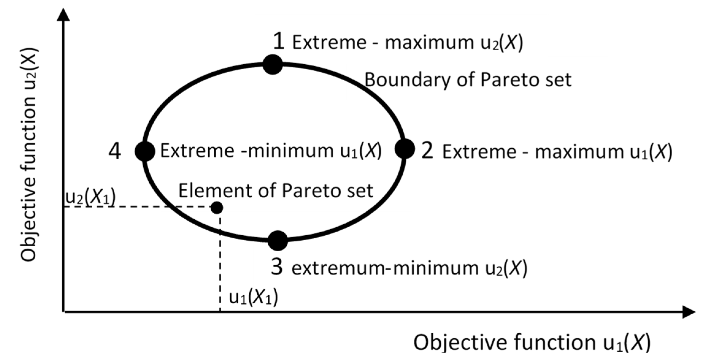
Multi-objective optimization by means of Pareto sets is based on search for boundary values of objective functions dependent on the same variable X of these functions. Values of objective functions are evaluated for every value of the independent variable X and plotted in the graph (see Figure 1). An element of Pareto set represents mutual relation of all considered objective functions for one given value of the independent variable X.
In the case of multi-objective optimization with two objective functions, Pareto sets have the form of plane graphs. One axis represents values of the first objective function and the second one values of the second objective function, as shown in Figure 1. Corresponding pairs of both functions (for the same variable values X) create Pareto set as the area of the graph. The set area limits are bound to a defined condition range of an independent variable for each function. The bound of Pareto sets makes outer limits of achievable values of the objective functions.
Peak points of the bound (Points 1, 2, 3, and 4 in Figure 1) depict extremes (minimum, maximum) of one and the other objective functions. Parts of the boundary between extremes match optimal values of variable X, because if the extremes of both these functions are simultaneously required (e.g., maximum 1 for u2(X) and maximum 2 for u1(X)), the extreme is achievable only for the first or second function. The change on Pareto boundary when dropping under the extreme of the first function approximates in the optimal way the solution to the extreme of the second function (for each variable X, between 1 and 2, both functions reach their maximum values). All variables X on Pareto boundary between these two extremes (Pareto-optimal front) are optimal (the most appropriate) because it is not possible to decide which combination of both objective functions is better. None of these solutions is worse or better—the solutions are mutually non-dominant.
In the case that the extreme of one function is also the extreme of the second function (for one value of the variable X, both extremes are reached) then Pareto-optimal front passes at one point (e.g., extremes 1 and 2 are identified) and the multi-objective optimization is one optimal solution only.
The goal of optimization is to find a non-dominant solution that requires the functions to be in contradiction (conflict). A change of variable X for one function towards its required extreme value delays the second function from its required minimum/maximum. A more detailed description of multi-objective optimization by means of Pareto sets can be found in literature [16] or [17].
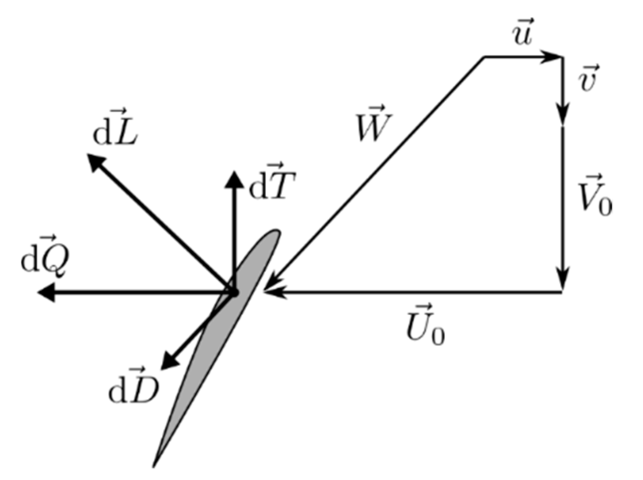
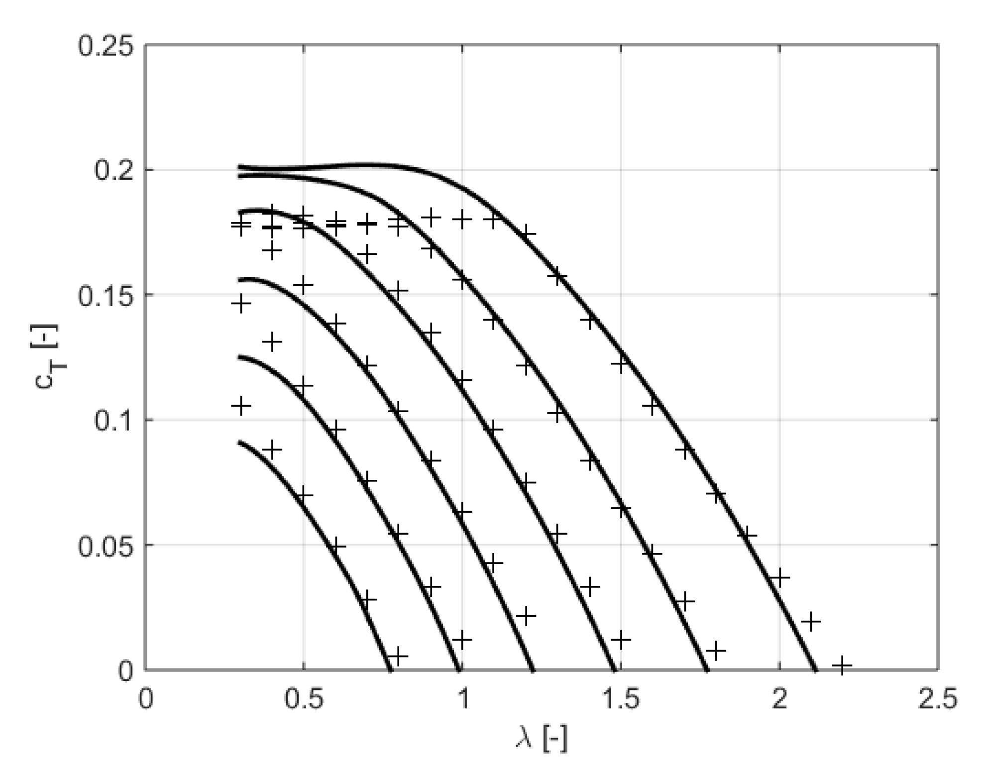
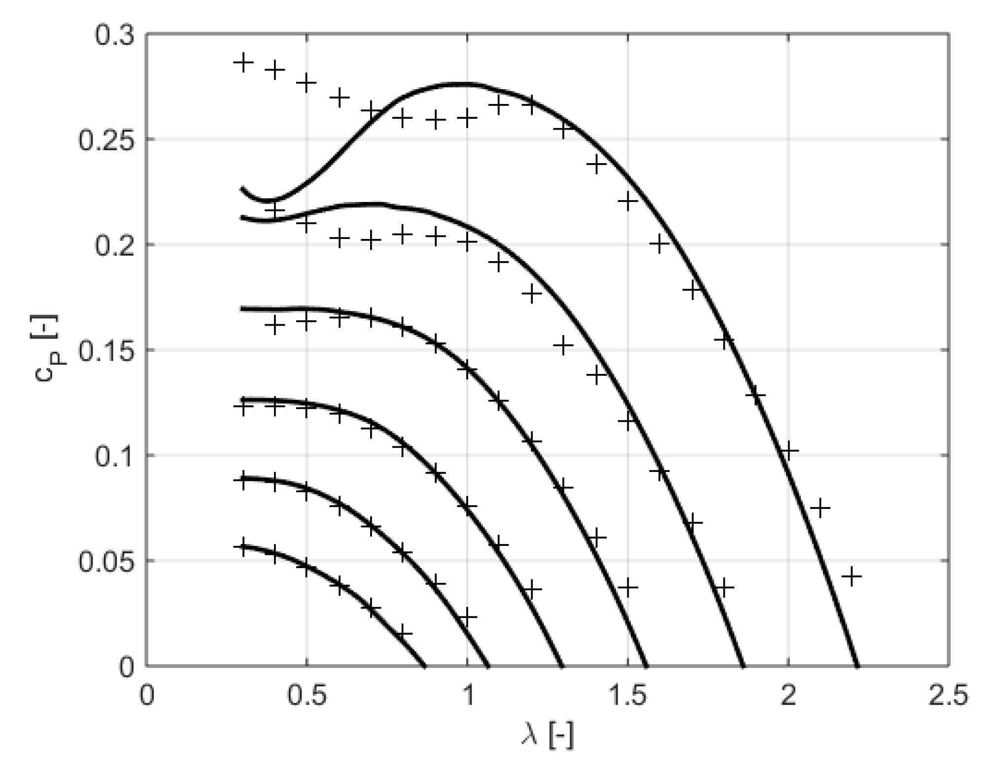
In the optimization selection of propellers from the family of propeller, the discrete points represent individual propellers. The propeller geometry comprises both continuously geometric parameters (mainly distribution of the chord length, twist and thickness of the airfoils used along the blade, the propeller diameter) and discrete parameter—the number of blades. The propeller aerodynamic characteristics represent the dependence of the thrust and power coefficients on the advance ratio (cT(λ), cP(λ)) that together with an engine power curve enables to set the available isolated thrust curve of the power unit.
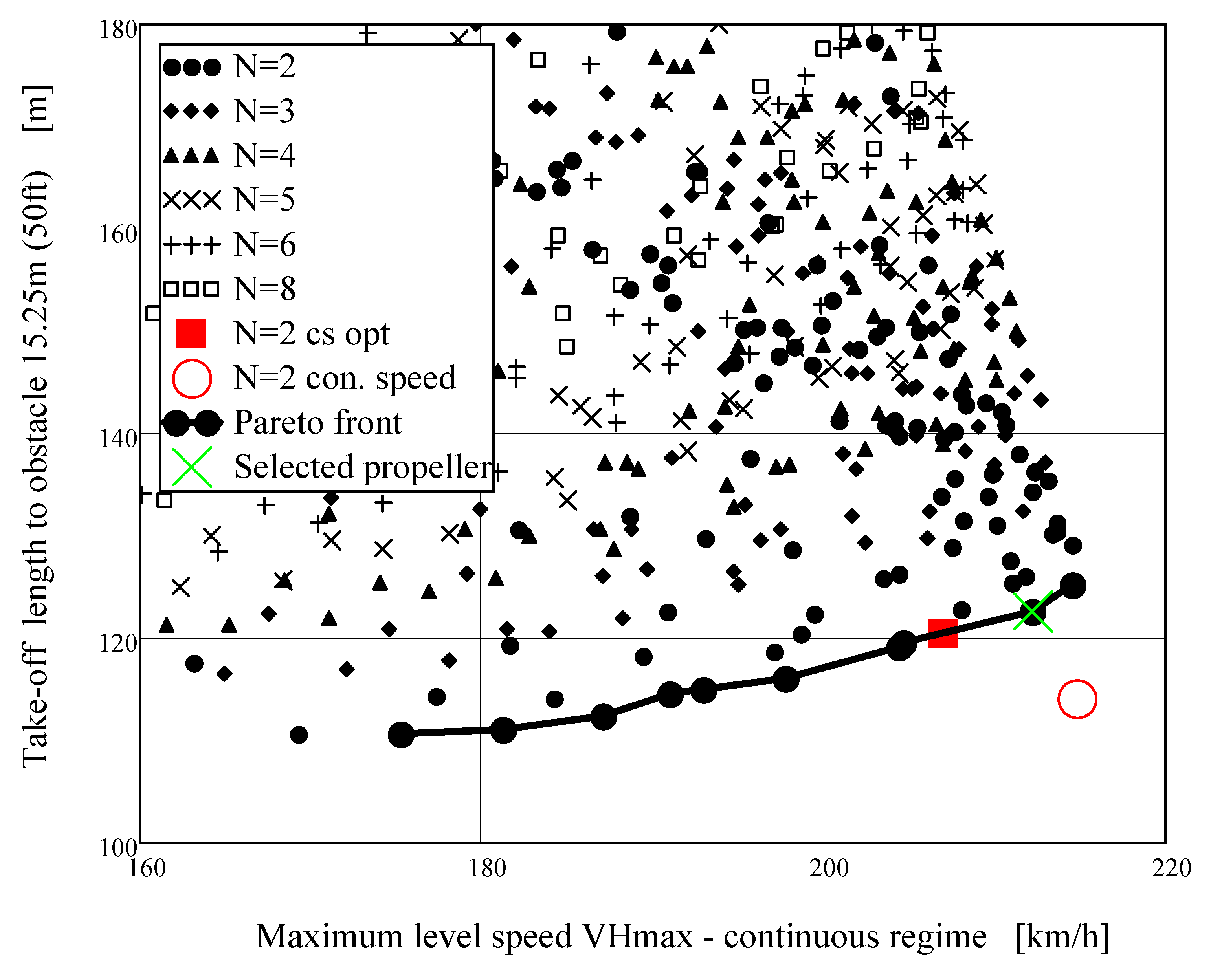
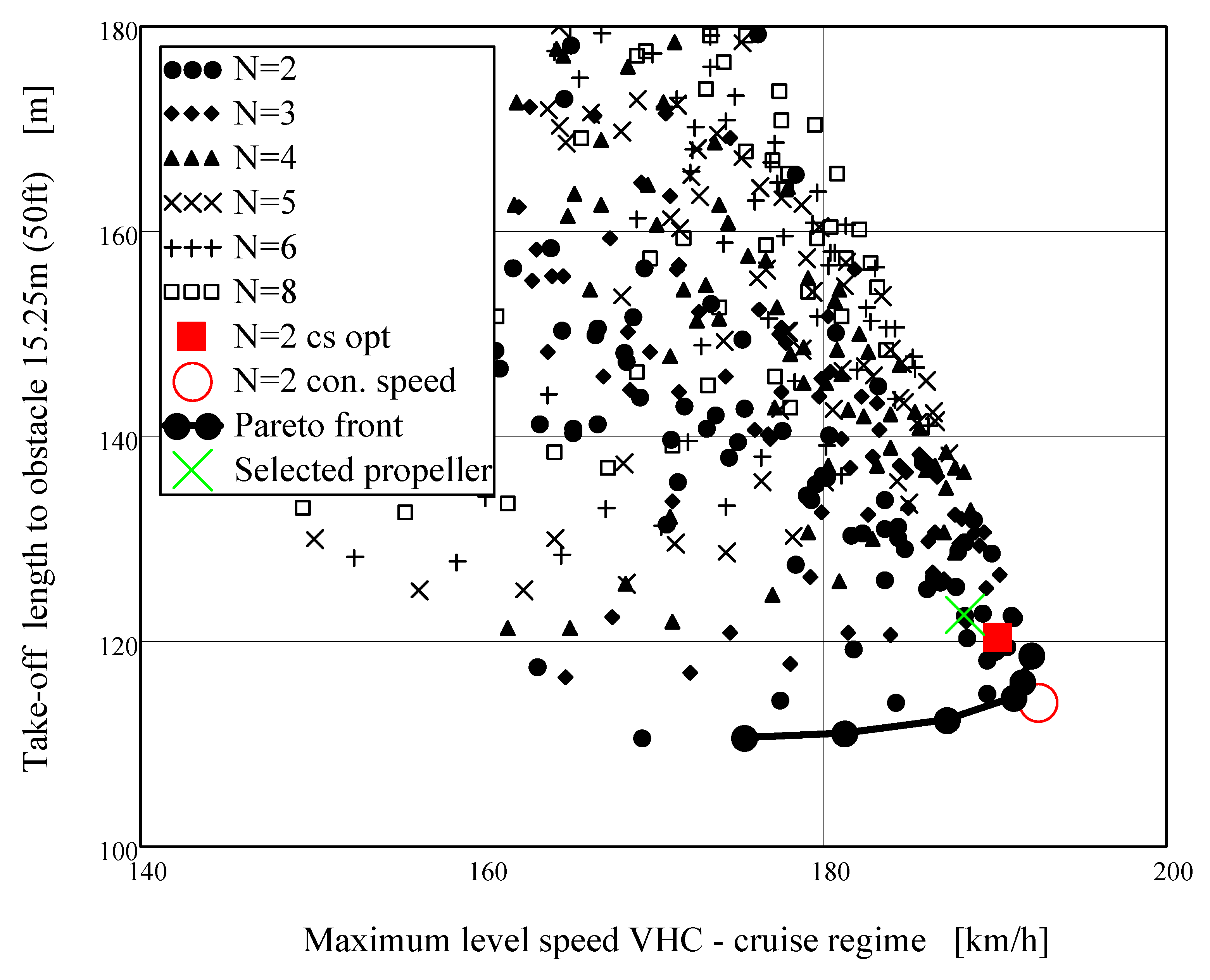
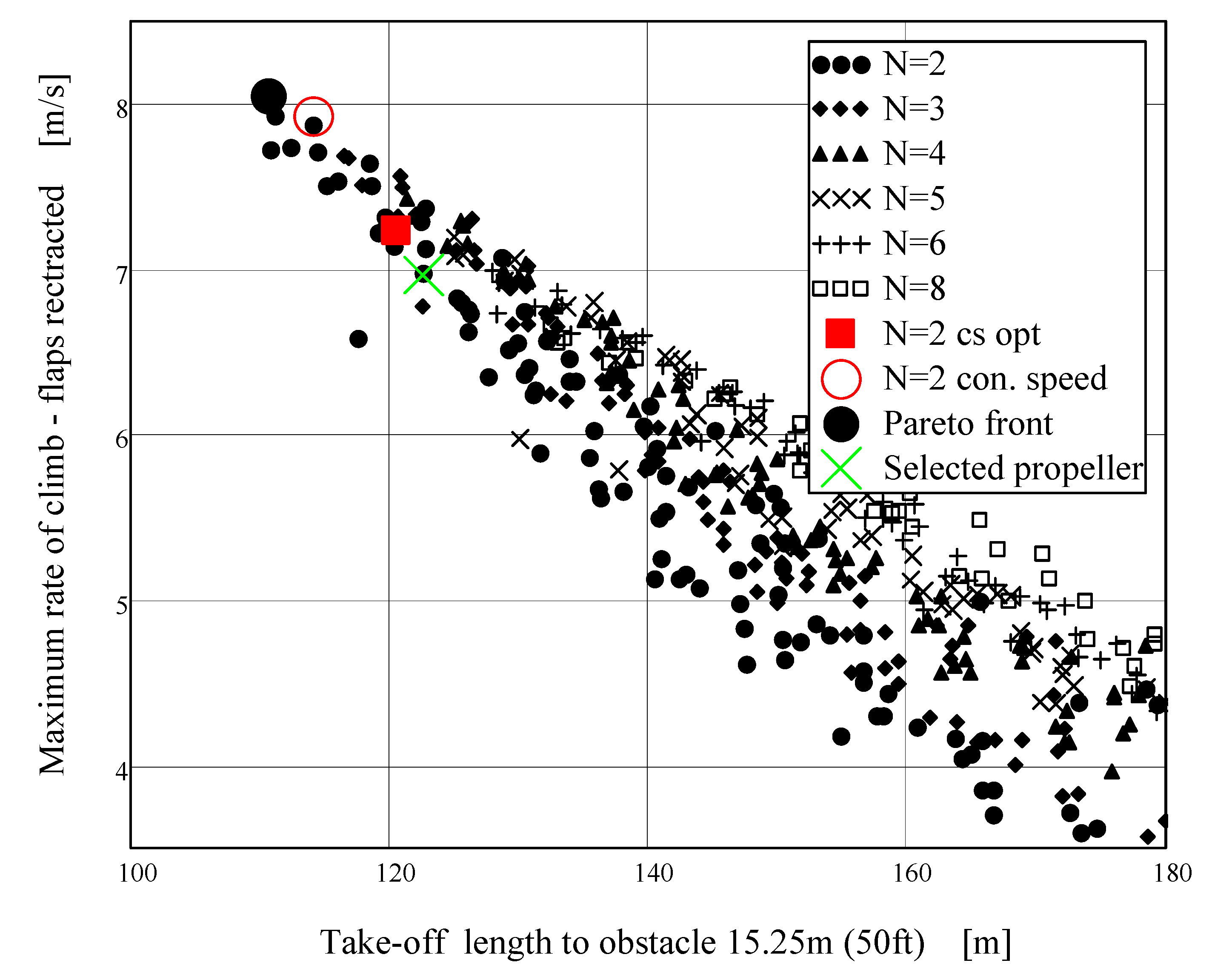
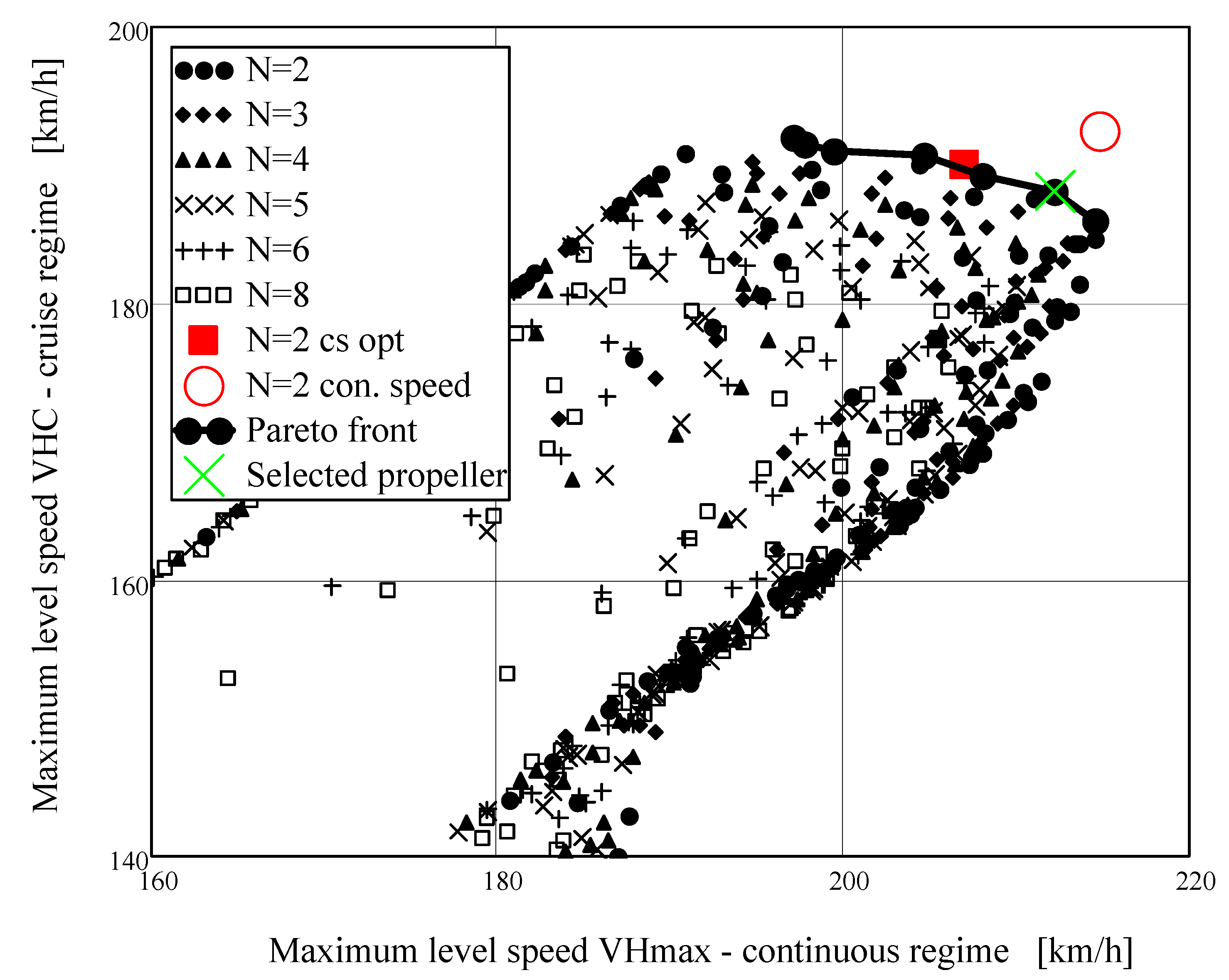
Pareto sets are composed from final number of points (equal to the number of propellers in the family of propeller) of appropriate pairs of the contradictory flight conditions objective functions: [maximum horizontal flight speed–take-off distance], [maximum horizontal flight speed–maximum rate of climb], [take-off distance–maximum rate of climb]. The pair of [maximum horizontal flight speed (continuous engine regime)–maximum horizontal flight speed (cruise regime)] is also included.
The optimization selection of the propeller by means of Pareto-optimal sets consists of the following sequential actions:
  • Assessment of free flight aerodynamic characteristics of the airplane (lift curve cL(α), lift-drag polar cL(cD) without the propeller influence on the airplane drag in the relevant flight configuration of the flight performance.
  • Determination of propeller aerodynamic characteristics—thrust and power coefficients cT(λ), cP(λ).
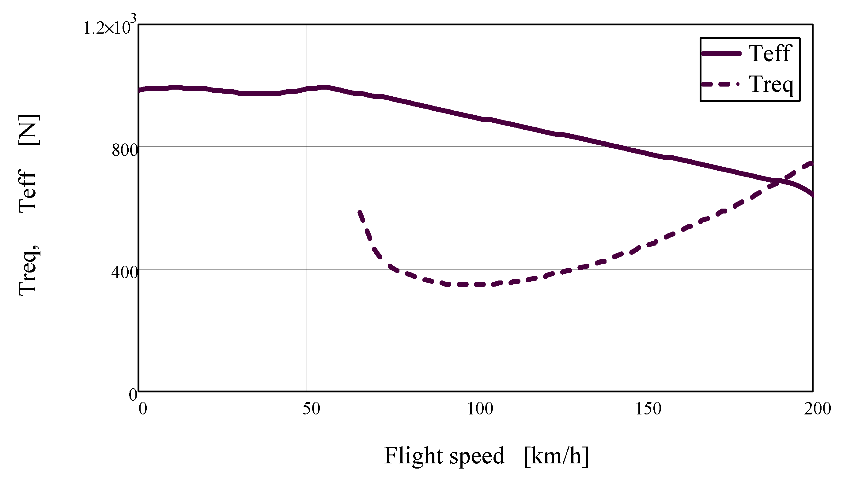
  • Calculation of the isolated thrust curve Tis(V) corresponding to the flight condition with the given engine regime, Tis(V) correction to the true T(V) and effective thrust Tef(V).
  • Calculation of all flight performance with the free airplane aerodynamic characteristics corrected for the respective ground effect of each flight condition.
  • Set up of the contradictory pairs of the flight conditions and creation of Pareto set graphs.
  • Evaluation of optimal Pareto fronts on Pareto sets graphs as the optimization selection.

3.2. Aerodynamic Characteristics of the Aeroplane

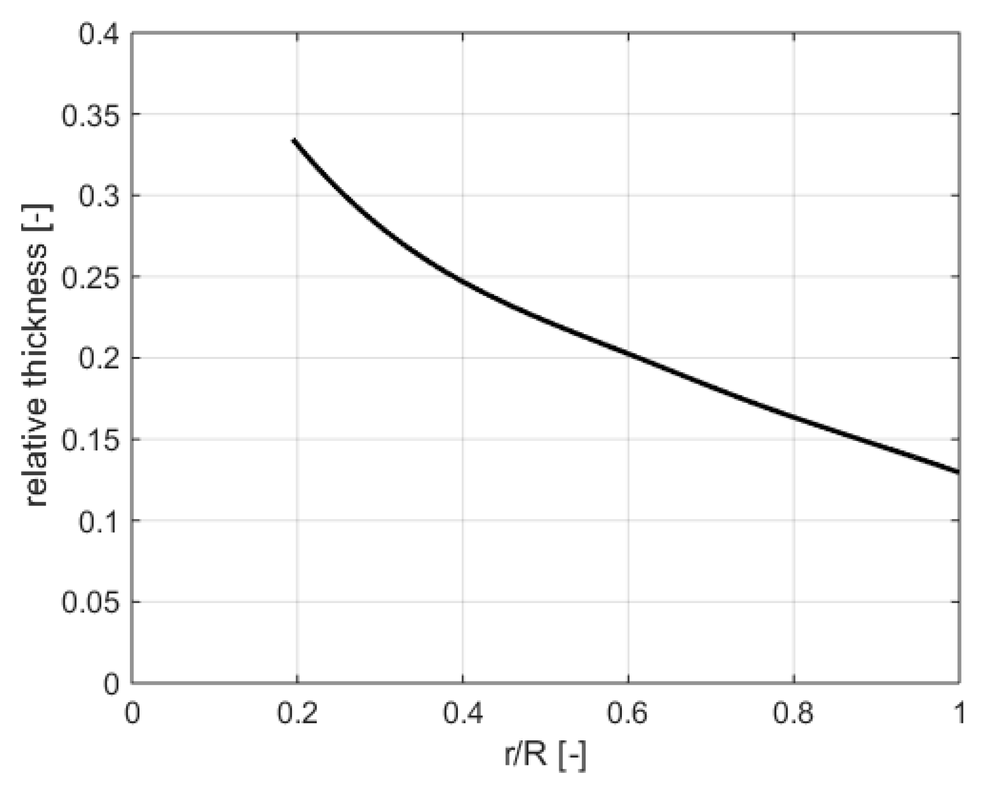
A model study of a small two-seat sport airplane with a requirement for a short take-off and landing (STOL) was chosen. The airplane is designed as the high-wing arrangement in which 13 m2 trapezoidal wing of the aspect ratio equals to 7.2. The wing is equipped with a combined high-lift device on the leading and trailing edge—a slotted leading edge (slat) and Fowler flap. The whole wing leading edge is equipped with slat; Fowler flap is installed on 60% of the wing trailing edge. Wing airfoil was developed from GA(W)-1 in order to increase lift coefficient. The airplane is drawn up with the standard side-by-side seat arrangement and a fixed taildragger landing gear with fairing.
Lift and drag aerodynamic characteristics were determined according to the methodology described in Appendix B for the following flight lift device configuration:
  • Take-off lift configuration—slat + Fowler flap 15°.
  • Cruise configuration—retracted lift devices.
The primary characteristics are determined without the propeller influence on the aerodynamic drag of the airplane and without the ground effect (see Figure 2). The characteristics correspond to moment-balanced states in the typical flight configuration. The primary lift and drag characteristics of take-off and landing configurations are corrected for the ground effect depending on the actual height above the ground. An additional airplane aerodynamic drag due to the propeller stream is included in the true propeller thrust.

3.3. Powerplant

The ROTAX 912 Aircraft Engine has been selected. The engine, primarily designed for this category of airplane, has take-off power of 73.5 kW and is equipped with a propeller speed reduction unit with gear ratio i = 2.43. The take-off regime corresponds to a maximum power at maximum permissible revolution per minute (RPM) for a short-term use, maximum 5 minutes (i.e., 5800 RPM at engine shaft); the continuous regime is 90% of the take-off power at reduced engine RPM (i.e., 5500 RPM at engine shaft) without any time limit; and the cruise regime (economic engine operation) means 75% of the continuous regime.

3.4. Propellers

3.4.1. Propeller Family

The propeller family is created as a group of geometrically similar propellers. Propeller blade geometry is derived from a three-blade propeller suitable for a 73.5 kW (100 hp) piston engine. The three-blade propeller was extended to other numbers of blades: two-blade, four-blade, five-blade, six-blade and eight-blade propeller with eleven pitch blade angles from 15° to 40° at 75% of radial distance. Geometric characteristics of the propeller are presented in Figure 3 (blade-chord distribution), Figure 4 (blade twist distribution) and Figure 5 (relative airfoil thickness). Clark Y airfoil is used. Range of propeller diameter of the total propeller family was from 1.1 m to 2.65 m, but each number of blades for a given pitch blade angle is only a part of this range. An extremely overloaded propeller that reaches the permissible engine RPM practically at the beginning of the take-off limits the smallest diameter. The maximum diameter represents a very lightly loaded propeller, and thus, the take-off is unacceptably extended, and the climbing rate is reduced.

3.4.2. Aerodynamic Characteristics of Propellers

Aerodynamic characteristics of propellers needed to determine thrust curves are dependencies of the thrust and power coefficients on the advance ratio, i.e., cT(λ) and cP(λ). The vortex blade theory of an isolated propeller is used. Free helix vortex surfaces with a constant pitch leaving the boundary vortex of each blade generate a field of the induced velocities that adjust the magnitude and direction of free flow along the propeller blade. The aerodynamic forces acting along the blade can be considered as two-dimensional airfoil characteristics with the incoming free flow corrected to the induced angle of attack. The calculations of the propeller aerodynamic characteristics were performed using the numerical model [18,19]. Input geometric data involve, except diameter D and number of blades N, also the distribution of the chord length, twist and thickness of the airfoils used along the blade. The calculation was done for every blade pitch setting and number of blades. More detailed description of the method can be found in Appendix A.

3.5. Thrust Curves of the Propeller

The thrust curve of the power unit has the meaning of the thrust available in dependence on flight speed. First, the thrust curves of the isolated propellers were calculated, and then, these isolated thrusts were corrected for influence of the installation. The corrected thrust represents the true thrust. Because the additional drag of the airplane (both friction and pressure part) due to the increased speed of the propeller stream is thus dependent on the propeller thrust, it is preferable for the calculations of the flight performance to introduce so-called effective thrust. The effective thrust is the true thrust reduced by the additional propeller drag. The drag curve of the airplane without the additional propeller drag thus remains the same for all alternatives of the propeller propulsion units. The friction component depending on the thrust and wetted area influenced by the propeller flow was evaluated according to literature [20].

3.6. Flight Performance for Pareto Sets

Aircraft performance is computed by methods described in [6] and [21]. More detailed explanation can be found in Appendix B. Computation is performed for 0 meters international standard atmosphere (ISA), i.e., air pressure 101,325 Pa, air density 1.225 kg·m−3 and air temperature 288.15 K (15 °C). Pareto sets require the pairing of such requirements, which are contradictory. The respective pairs of flight conditions required to achieve their extreme values (minimum, maximum) act on each other so that increasing one flight condition towards the extreme decreases the second flight condition from its desired extreme.
In general, it can be expected that the propellers with good take-off performance are not good for reaching maximum flight speeds and vice versa. Therefore, for pairs of the flight conditions for Pareto set, the following are used:
  • Maximum horizontal flight speed (continuous engine regime)–Take-off distance (take-off engine regime).
  • Maximum horizontal flight speed (cruise engine regime)–Take-off distance (take-off engine regime).
  • Maximum horizontal flight speed (continuous engine regime)–Maximum rate of climb (take-off engine regime).
  • Maximum horizontal flight speed (cruise engine regime)–Maximum rate of climb (take-off engine regime).
  • Take-off distance (take-off engine regime)–Maximum rate of climb (take-off engine regime).
  • Maximum horizontal flight speed (continuous engine regime)–maximum horizontal flight speed (cruise regime).

4. Results

Pareto sets of six-selected flight condition pairs discussed in the Section 3.6 are plotted in Figure 6, Figure 7, Figure 8, Figure 9, Figure 10 and Figure 11. Every point in the graph represents aircraft performance for one propeller defined by its number of blades, diameter and blade angle setting. Flight performance is computed according to the methodology described in Section 3. Marker types depend on the number of blades. For clarity, only limited areas near Pareto-optimal fronts from the all propeller family combinations are depicted. The broken lines connect points from Pareto-optimal fronts. Selection by means of speed power coefficient cs is used for comparison (see cs opt points in Figure 6, Figure 7, Figure 8, Figure 9, Figure 10 and Figure 11). Performance with original constant-speed propeller is also shown for comparison. Results are further discussed in Section 5. Table 1, Table 2, Table 3, Table 4, Table 5 and Table 6 contain coordinates of the points on the Pareto fronts for corresponding Pareto graphs. Pareto fronts are formed only by two-blade propellers; propeller diameter and blade angle are mentioned for every point. Performance with selected optimal propeller is also plotted in Figure 6, Figure 7, Figure 8, Figure 9, Figure 10 and Figure 11).
Figure 6 shows Pareto set for the Maximum level speed (continuous engine regime) vs. take-off length. Pareto front is located in the lower right-hand corner (short take-off and maximum speed). Pareto front is created uniquely by two-blade propellers. Two-blade propeller optimized by the means of the power speed coefficient cs is on the Pareto-optimal set. Figure 7 shows similar situation for the cruise speed. In this case, Pareto-optimal set contains also uniquely two-blade propellers, but the solution obtained by the means of the speed power coefficient is no more on the Pareto-optimal set.
Figure 8 and Figure 9 present Pareto-optimal front for the cases maximum level speed (continuous engine regime) vs. rate of climb and cruise speed vs. rate of climb. Both parameters should be maximal, i.e., optimal solutions are in the top right-hand part of the graph. Like before, optimal solution obtained by means of speed power coefficient is part of optimal set only for the case of the maximal continuous engine power.
Figure 10 presents Pareto frontier for the combination of take-off length vs. rate of climb. Optimal set is created only by single point in this case. Figure 11 presents Pareto frontier for the combination of maximum level speed (continuous regime) vs. cruise speed. Both parameters should be maximal, so the optimal set is located in the top right-hand part of the graph. As in previous cases, optimal set is represented only by two-blade propellers. Optimal solution obtained by means of the power speed coefficient is the part of this set.

5. Selection of Optimal Propeller

Optimal propeller is selected from the group of near to the Pareto fronts in the Figure 6, Figure 7, Figure 8 and Figure 9 and Figure 11. The choice itself depends on the weight factors given to the different parameters, i.e., trade-off is always necessary. Take-off length was selected as the most important parameter due to the STOL category aircraft. Weight factors can be of course modified and tuned according to the designer requirements. The selected optimal propeller has two blades, diameter D = 2.05 m and pitch blade angle ϕ0.75 = 20°. This point is part of the Pareto fronts in Figure 6, Figure 8 and Figure 11. It is also close to the Pareto front in other cases. Aircraft performance with the optimal propeller is described in Table 7.

6. Conclusions

Multi-objective optimization using Pareto sets of flight performance of 472.5 kg small STOL sport airplane powered by 73.5 kW (100 hp) engine to select a fixed propeller from a family of geometrical similar propellers is presented. The propeller family included propellers from two-blade to eight-blade with pitch blade angles from 15° to 40° and diameters range from 1.1 m to 2.65 m.
The optimization criteria required maximum level speed, maximum rate of climb and minimal take-off. The optimal Pareto fronts were investigated for four pairs of opposing flight conditions:
  • Maximum horizontal flight speed–Take-off distance.
  • Maximum horizontal flight speed–Maximum rate of climb.
  • Take-off distance–Maximum rate of climb.
  • Maximum horizontal flight speed–maximum horizontal flight speed (cruise regime).
Length of take-off path and maximum rate of climb relate to the take-off engine power regime; maximum horizontal flight speed was considered for both continuous and cruise power regime. Only four pairs of parameters are used for the optimization due to the fact that the last two pairs (take-off distance vs. rate of climb and cruise speed vs. maximal horizontal speed) in fact do not affect the choice of the optimal propeller.
Pareto-optimal study leads to the following conclusions:
  • Only two-blade propellers belong to all Pareto-optimal fronts.
  • One cut-off point of Pareto-optimal fronts for maximum horizontal speed corresponds to D = 1.95 m, pitch blade angle ϕ0.75 = 22.5° for the continuous engine regime and to D = 2 m, ϕ0.75 = 20° for cruise regime.
  • The opposite cut-off points of Pareto-optimal front for both maximum rate of climb and minimal take-off distance corresponds one propeller: D = 2.1 m, pitch blade angle ϕ0.75 = 15°.
  • The constant speed propeller achieves better performance than the best performance of the fixed pitch and ground adjustable propellers for all four optimization criteria.
Acceptable aircraft performance is reached for the propellers with two blades, diameter in the range from D = 1.95 to 2.2 m with a corresponding decrease of blade angle from ϕ0.75 = 22.5° to 12.5°. Optimal propeller is then selected from this group.
To compare Pareto multi-objective optimization with standard selection propeller from a family of geometrically similar propellers by means of the speed power coefficient, the design was performed for design speed from the middle of Pareto-optimal front of maximal horizontal speed for continuous engine regime. The single-mode optimization selection for two-blade propeller confirms Pareto optimization selection: diameter D = 2.05 m and pitch blade angle ϕ0.75 = 20°. The speed power coefficient methods are limited by single-regime design defined by given flight speed and engine regime, and the design is not clearly connected to flight performance. Two-blade propeller of this family considered as a constant speed propeller with diameter obtained by the speed power coefficient presents an increase in flight performance for the fixed pitch propeller.

Author Contributions

Author contributions are divided in the following way: conceptualization, S.S. and J.B.; methodology, J.K.; software, S.S. and J.K.; validation, S.S. and J.B.; formal analysis, S.S.; writing—original draft preparation, S.S. and J.K.; writing—review and editing, J.K.; visualization, S.S.; supervision, J.K. All authors have read and agreed to the published version of the manuscript.

Funding

This work was supported by the EU Operational Programme Research, Development and Education, under the Centre of Advanced Aerospace Technologies, project No. CZ.02.1.01/0.0/0.0/16_019/0000826, Faculty of Mechanical Engineering, Czech Technical University in Prague.

Conflicts of Interest

The authors declare no conflict of interest.

Nomenclature

DPropeller diameter, Drag
HAltitude
LLift
NNumber of propeller blades
PEngine power
PmaxMaximum engine power
QTangential force
SWing area
SPPropeller disc area
SwetAircraft area wetted by the propeller flow
TTrue propeller thrust
TeffEffective propeller thrust, Teff = (T − ΔD)
TisIsolated propeller thrust
TreqRequired thrust
U0Rotational flow speed on the propeller (freestream)
VFlight speed
V0Axial flow speed on the propeller (freestream)
VHmaxMaximum horizontal flight speed–continuous engine regime
VHCMaximum horizontal flight speed–cruise engine regime
VminStalling speed
V1Safe lift-off speed
V1PFlow velocity through the propeller disc (actuator disc)
V2Safe take-off climb speed (Safe speed of transition)
WTotal flow speed on the propeller
ΔDAirplane drag induced by the propeller, ΔD = ∆Dfr + ∆Dpr
DfrFriction component of airplane-propeller drag
DprPressure component of airplane-propeller drag
RPropeller radius
cBlade chord
cPPower coefficient of the isolated propeller, cP = P/(ρ ns3 D5)
cTThrust coefficient of the isolated propeller, cT = Tis/(ρ ns2 D4)
csSpeed power coefficient of the isolated propeller, cs = [ρ V5/(P ns2)]1/5
cDDrag coefficient
cDminMinimum drag coefficient
cLLift coefficient
cLmaxMaximum lift coefficient
cLαLift-curve slope
fRolling friction coefficient
harcHeight of the transition arc
hWDistance of the wing under the ground
iGear ratio of the engine speed reducer
mAircraft weight
n, nmaxEngine speed, Maximum engine speed
nsPropeller speed per second
nyLift load factor
rRadial coordinate
uInduced tangential speed on the propeller
vInduced axial speed on the propeller
vyRate of climb
ηPropeller efficiency, η = cT λ/cP
λPropeller advance ratio, λ = V/(ns D)
λWWing aspect ratio
ρAir density
φ0.75Propeller pitch blade angle at 75% of the radial distance
ΩPropeller angular velocity
Abbreviations
ISAInternational Standard Atmosphere
STOLShort Take-off and Landing

Appendix A. Computation of Propeller Characteristics

Method for the computation of propeller characteristics is based on the combination of blade element theory and vortex theory. Dimensionless variables are used for the computation of isolated propeller performance. Standard formulations are used (see [19]). Flight velocity is expressed by advance ratio λ
λ = V n s D .
Thrust is expressed by thrust coefficient cT
c T = T ϱ n s 2 D 4 .
Power coefficient cP is defined in a following way
c P = N ϱ n s 3 D 5 .
Radial coordinate r is replaced by
r ¯ = r R ,
Dimensionless velocities are defined in a following way
U ¯ = U Ω R ,
and dimensionless circulation Γ ¯ is used in following form
Γ ¯ = Γ 4 π Ω R 2 .
Thrust and power coefficients can be determined from [19]
c T = π 3 r ¯ 0 1 Γ ¯ ( U ¯ 1 c D c L V ¯ 1 ) d r ¯ ,
c P = π 4 r ¯ 0 1   Γ ¯ ( V ¯ 1 + c D c L U ¯ 1 ) r ¯ d r ¯ .
Velocities on the propeller blade is shown in the Figure A1. U1 and V1 are defined by
U ¯ 1 = U ¯ 0 + u ¯ ,
V ¯ 1 = V ¯ 0 + v ¯ ,
where u and v represent induced velocities (during normal propeller operation, u is negative, and v is positive). Vortex theory is used for the determination of induced velocities. System of horseshoe vortices is used (see Figure A2). Induced velocities are computed by the way described by Okulov [22].
Figure A1. Flowfield and forces on the propeller blade.
Aerospace 07 00021 g0a1
Figure A2. Illustration of the vortex system on the propeller blade.
Aerospace 07 00021 g0a2
Lift coefficient cL is coupled with circulation by
Γ ¯ = 1 2 c L N c ¯ W ¯ 1 .
Airfoil section lift and drag coefficients are computed by means of the mathematical model described in [23]. Iterative procedure in MATLAB environment is used for the solution of the system of equations. The procedure was tested on the case of the three-blade propeller 5868-R6 described in [8]. Comparison of the computed results with experimental data is presented in Figure A3 and Figure A4.
Figure A3. Comparison of computed values of thrust coefficient cT (solid lines) with experimental results from [8] (discrete points) for the three-blade propeller 5868-R6.
Aerospace 07 00021 g0a3
Figure A4. Comparison of computed values of power coefficient cP (solid lines) with experimental results from [8] (discrete points) for the three-blade propeller 5868-R6.
Aerospace 07 00021 g0a4

Appendix B. Computation of Flight Performance

Appendix B.1. Thrust Curve of the Propeller Power Unit

The thrust curve of the power unit has the meaning of the available thrust in dependence on flight speed. First, the thrust curves of the isolated propellers are calculated, and then, the isolated thrust is corrected for influence of the installation. The corrected thrust represents the true thrust.
Because the additional drag of the airplane (both friction and pressure part) due to the increased speed of the propeller stream depends on the propeller thrust, it is preferable for the calculations of the flight performance to introduce so-called effective thrust. The effective thrust is the true thrust reduced by the additional propeller drag. The drag curve of the airplane without the additional propeller drag thus remains the same for all alternatives of the propeller propulsion units.

Appendix B.1.1. Thrust of Isolated Fixed-Pitch and Ground-Adjustable Propellers

Determination of the thrust curve of an isolated propeller requires, as the first step, the solution of the equilibrium propeller–engine rotational speed:
P ( n ) = ρ ( H ) n s 3 D 5 c P ( λ ) .
The solution determinates the root of the power equation expressed by the engine power curve P(n) on one side and the propeller power described by the power coefficient cP(λ) for a given flight speed V on the other side. The equilibrium speed is solved for a number of speeds from the full range of the flight speed. The pair of the flight speed and the equilibrium rotational speed determinates the advance ratio λ and by help of the thrust coefficient cT(λ) the isolated thrust can be evaluated:
    T i s = ρ ( H ) n s 2 D 4 c T ( λ ) .
The power engine curve P(n) pertains to one of the three engine regimes: Take-off, Continuous and Cruise.
In the case that the equilibrium rotational speed with an increasing flight speed reaches the maximum allowed value nmax, it is assumed that the pilot will maintain this limit rotational speed by the throttle. The equilibrium rotational speed in such overload regime is thus the maximum speed nmax.

Appendix B.1.2. Thrust of Isolated Constant-Speed Propellers

As the constant-speed propeller keeps the rotational speed constant independently of the flight speed, then, the regulated rotational speed is actually the equilibrium speed. It is therefore possible to calculate the thrust directly by means of the thrust coefficient curve cT(λ) determined for the constant-speed propeller working in the required power regime.

Appendix B.1.3. Thrust Curve with Influence of Height

For calculating of thrust curves at different heights, the engine power of the piston engine at zero altitude can be converted to the given height H by a multiple factor kN according to [24]
k N ( H ) = ( 1 + 0.132 ) ρ ( H ) ρ 0 0.132   .      
The air density ρ at height H [m] corresponds to the standard dependence according to ISA:
ρ ( H ) = ρ 0 ( 1   H 44308 ) 4.256   ,
where
  ρ 0 = 1.225   kg / m 3   ,
and the constant 44,308 m represents the ratio of two individual constants: the constant temperature decreases with high 0.0065 K/m and temperature of 288 K for H = 0 m.
The influence of the height on aerodynamic characteristics of propellers can be neglected.

Appendix B.1.4. True Thrust of Installed Propellers

The ratio of the true propeller thrust T and the thrust of isolated propeller Ti is estimated as the ratio of the actuator disc thrust of the propeller with a mean flow speed through the disc and thrust of the isolated actuator disc. The mean flow speed corresponds to the deceleration downstream due to a body behind the propeller. The mean value of the decelerated flow through the disc is determined from the equality of the flow momentum by the actuator disc with a constant and variable velocity.
The graphical dependence published in [19] is used to describe the change of the speed in the plane of the propeller disc caused by an engine nacelle. The graph shows the relative velocity drop (ΔV1P/V1P) in the plane of the propeller disc in the area of the central part of the propeller. The central part is defined by the cross-section of the engine nacelle Sn. The velocity drop ratio depends on the cross-sectional area Sn and propeller disc area SP and a compensatory analytical form of the graph has the form:
Δ V 1 P V 1 P = 0.2 S n S P 0.08 S n S P + 0.028   .  
The ratio of the thrusts is determined from the momentum of the induced velocity of the ideal actuator disc in the steady-state distance behind the disc and momentum of the ideal actuator disc with the mean speed. The ratio determinates the final correction factor to convert the isolated thrust to the true thrust:
k i s = ( 1 S n S P ( Δ V 1 P V 1 P ) ) 2 V 1 P ( 1 S n S P ( Δ V 1 P V 1 P ) ) V 2 V 1 P V   .
The flow velocity V1P through the propeller disc can be expressed depending on the thrust at flight speed V according to the theory of the ideal actuator disc:
V 1 P = V 2 ( 1 + 1 + T i s 1 2 ρ ( H ) S P V 2 )   .  
In the case of the single-engine airplane, the nacelle cross-section Sn is replied by the cross-section area of the engine part of the fuselage.

Appendix B.1.5. Effective Thrust

The effective thrust means the true propeller thrust reduced by the additional airplane drag generated by the propeller stream consisting of a friction and pressure component:
T e f f = T ( Δ D f r Δ D p r ) .
The friction component ∆Dfr is depended on the thrust and a wetted area of an airplane influenced by the propeller flow. Its mean value is presented in References [20,24]:
Δ D f r = 0.004   T S w e t S P .
The pressure component ∆Dpr is taken from Reference [19] for the engine nacelle case:
Δ D p r = Δ V 1 P V 1 P   T .  
The conversion factor of the true trust to the effective thrust can thus be expressed in the form:
k e f f = 1 0.004 ( S w e t S P ) 0.2 S n S P 0.08 S n S P + 0.028   .

Appendix B.2. Curves of Available and Required Thrust and Power

Appendix B.2.1. Available Thrust Curve

The available thrust represents the effective thrust Teff; see (A20). The available thrust curve is the dependence of the effective thrust on the flight speed V.

Appendix B.2.2. Required Thrust Curve

The required thrust is equal to the thrust that corresponds to the aerodynamic drag force without additional drag caused by propeller in a balanced horizontal flight at a steady flight speed V.
Calculation procedure for determining the required thrust:
  • Step 1: To determine the needed lift coefficient from the balance of lift and weight for the chosen flight speed V:
  c L = m g 1 2 ρ ( H ) V 2 c L S     .  
  • Step 2: To state the corresponding drag coefficient from the aerodynamic polar of the respective flight configuration (without additional aerodynamic drag caused by propeller flow) for the corresponding lift coefficient. Drag coefficient cD is determined from aerodynamic polar (Figure 2).
  • Step 3: The required thrust is equal to the aerodynamic drag:
T r e q = 1 2 ρ ( H ) V 2 c D S .
Steps 1–3 shall be repeated from Vmin (minimum horizontal flight speed at the given configuration–stalling speed) to the maximum flight speed VHC (or VHmax) corresponding to the intersection of the required thrust curve Treq(V) with the available thrust curve Teff (V) for a given altitude. An example of the curve of available and required thrust of a small sport aircraft at a cruise regime is depicted in Figure A5.
Figure A5. Curves of available and required thrust for a small sport aircraft m = 473 kg at a cruise configuration with three-blade propeller: D = 1.75 m, φ0.75 = 22°, maximum cruise-regime power 47.9 kW.
Aerospace 07 00021 g0a5
Stalling speed:
V m i n = m g 1 2 ρ ( H ) V 2 c L m a x S   .
Maximum flight speed: see (A31).

Appendix B.2.3. Required Thrust Curve with Influence of Height

1. Ground influence
Due to the ground proximity, aerodynamic drag decreases and lift increases. A simple correction according to Reference [21] is introduced for induced part of the drag and the lift-curve slope:
  c D g r o u n d = c D m i n + ( 1 σ ) ( c D c D m i n )   ,  
where the correction factor σ is dependent on the height hW of the wing above the ground, the aspect ratio of the wing λW and its area S:
σ ( h W , λ W , S ) = e   [ 4.22 ( h W λ W S ) ] 0.768 ,  
c L g r o u n d = c L π λ W [ ( 1 σ ) c L α ]   .
2. Out of ground influence
Changes of aerodynamic forces are considered only by changing of the air density with height. The effect of Reynolds number changes on aerodynamic coefficients is neglected.

Appendix B.2.4. Available Power Curve

    P e f f ( V ) = T e f f ( V )   V .

Appendix B.2.5. Required Power Curve

    P r e q ( V ) = T r e q ( V )   V .

Appendix B.3. Maximum Horizontal Speed, Maximum Rate of Climb

Standard calculation models based on the curves of the required and available thrust and power are used to determine the maximum horizontal speed and maximum rate of climb; see, for example, Reference [20].
Maximum flight speed:
  T r e q ( V ) = T e f f ( V )       V = V H C .
Flight speed of maximum rate of climb Vvymax:
  ( P e f f ( V ) P r e q ( V )   ) = max     V = V v y m a x   .
Maximum rate of climb:
v y m a x =     P e f f ( V v y m a x ) P r e q ( V v y m a x )     m g   .

Appendix B.4. Take-Off Distance

The take-off distance is understood to be the horizontal distance of the classic take-off procedure consisting of the ground round phase and three airborne phases: the ground flight, transition and climb out. The standard dynamic models of the take-off, discussed in, e.g., References [20,25], are adopted for the individual phases. The normal take-off considers the airplane with the take-off configuration of the lift device.

Appendix B.4.1. Take-Off Ground Run

The take–off ground run determines the distance to achieve the safe lift-off speed V1.
Length of the ground run:
L 1 = 0 V 1 V R g r o u n d   r u n ( V ) d V     ,
where safe lift-off speed V1 is within the range (110–115)% of the stall speed with the ground effect. Stalling speed with the ground run effect corresponds to the relationship (A26):
      V m i n _ g r o u n d   r u n = m g 1 2 ρ ( H ) V 2 c L m a x _ g r o u n d   r u n   S   ,
                for :     c L m a x g r o u n d   r u n = c L m a x π λ W [ ( 1 σ ( h W g r o u n d   r u n , λ W , S ) ) c L α ]   .
Rground run represents an accelerating force during the ground run:
R g r o u n d   r u n ( V ) = T e f f ( V ) m g f ( c D g r o u n d   r u n c L g r o u n d   r u n   f ) 1 2 ρ ( H ) V 2 S   ,
with such a take-off angle of attack that satisfies the optimal condition:
d c L g r o u n d   r u n d c D g r o u n d   r u n = 1 f   .
Tangent to the lift-drag at the ground run point is equal to the inverse value of the rolling friction coefficient 1/f.

Appendix B.4.2. Take-Off Ground Flight

The take–off ground flight corresponds to the acceleration phase of the ground level flight from the safe lift-off speed V1 up to the safe take-off climb speed V2.
Length of the ground flight:
L 2 = V 1 V 2 V R g r o u n d   f l i g h t ( V ) d V ,
where safe take-off climb speed V2 is required at least 120% of the stall speed in the ground flight regime. Stalling speed with the ground flight effect corresponds to the relationship (A26):
      V m i n _ g r o u n d   f l i g h t = m g 1 2 ρ ( H ) V 2 c L m a x g r o u n d   f l i g h t   S   ,
                for :     c L m a x g r o u n d   f l i g h t = c L m a x π λ W [ ( 1 σ ( h W g r o u n d   f l i g h t , λ W , S ) ) c L α ]   .
Rground flight represents an accelerating force during the ground flight:
R g r o u n d   f l i g h t ( V ) = T e f f ( V ) c D g r o u n d   f l i g h t ( V ) 1 2 ρ ( H ) V 2 S .
The aerodynamic coefficients correspond to the point on the lift-drag polar of the ground-run configuration (corrected to the ground effect) at which the lift coefficient is equal:
c L g r o u n d   f l i g h t ( V ) = m g 1 2 ρ ( H ) V 2   S   .
Both of these coefficients thus depend on the ground flight speed V.

Appendix B.4.3. Take-Off Transition

The take–off transition phase means a curved flight from the safe take-off climb speed to the transition straight climb. The transition is taken as a flight close to a vertical circular arc with a constant speed equal to the safe take-off climb speed V2.
Horizontal length of transition arc:
L 3 = r   s i n ( θ )   ,
where the radius of transition arc r deepens on the load factor ny caused by the curvilinear flight:
r = V 2 2 [ g ( n y c o s ( θ ) ) ]     .
The maximum achievable value of the load factor at the constant speed V2 is
n y m a x = ( V 2 V min _ g r o u n d   f l i g h t ) 2   .
This maximum value corresponds to the cLmax ground flight and leads to the shortest length of the take–off transition phase, but it is on the edge of the sharp flow separation. A smaller value ny should be considered, e.g., 80% nymax.
The output angle from the transition arc is given by the difference of the available and required thrust at the transition speed:
θ = a r c s i n [ T e f f ( V 2 ) T r e q ( V 2 ) m g ]   ,
where the required thrust equals:
T r e q ( V 2 ) = c D g r o u n d   f l i g h t ( V 2 ) 1 2 ρ ( H ) V 2 2 S .
As the ground effect during the transition flight is gradually decreasing, an approximate procedure based on a mean value height hW of the wing above the ground is applied. The mean value can be estimated, e.g., as a mean value between the height of arc harc calculated with the ground effect of the take-off ground flight and without the ground effect (free flight).
h W t r a n s i t i o n = 1 2 [ h a r c ( σ ( h W g r o u n d   f l i g h t ) + h a r c σ ( h W ) ) ] ,
where the arc height is equal:
h a r c = r [ 1 c o s ( T e f f ( V 2 ) T r e q ( V 2 ) ) ] .

Appendix B.4.4. Climb Out

The climb out is the phase of the steady climbing flight at the speed of the transition phase from the transition arc until the obstacle height hobs (usually 15.25 m = 50 ft)) is reached:
L 4 = h o b s ( h W g r o u n d f l i g h t + h a r c ) t g ( θ )   ,
where the arc height harc and take-off output angle θ are determined for hW_transition.

Appendix B.4.5. Total Take-Off Distance

Total take-off distance is equal to the sum:
L t a k e o f f = L 1 + L 2 + L 3 + L 4 .

References

  1. Betz, A. Schraubenpropeller mit geringstem Energieverlust. Göttinger Nachrichten 1919, 1919, 193–213. [Google Scholar]
  2. Goldstein, S. On the Vortex Theory of Screw Propellers. Proc. R. Soc. Lond. (A) 1929, 123, 440. [Google Scholar]
  3. Larrabee, E.E. Practical Design of Minimum Induced Loss Propellers. SAE Trans. 1979, 88, 2053–2062. [Google Scholar]
  4. Adkins, C.N.; Liebeck, R.H. Design of Optimum Propellers. J. Propul. Power 1994, 10, 676–682. [Google Scholar] [CrossRef]
  5. Hepperle, M. Inverse Aerodynamic Design Procedure for Propellers Having a Prescribed Chord-Length Distribution. J. Aircr. 2012, 47, 1867–1872. [Google Scholar] [CrossRef]
  6. McCormick, B.W. Aerodynamics, Aeronautics, and Flight Mechanics, 2nd ed.; John Wiley & Sons: Hoboken, NJ, USA, 1995. [Google Scholar]
  7. Hartman, E.P.; Biermann, D. The Aerodynamic Characteristics of Full-scale Propellers Having 2, 3, and 4 Blades of ClarkY and R.A.F. 6 Airfoil Sections; NACA Technical Report No. 640; Langley Memorial Aeronautical Laboratory: Hampton, VA, USA, 1938. [Google Scholar]
  8. Hartman, E.P.; Biermann, D. The Aerodynamic Characteristics of Six Full-scale Propellers Having Different Airfoil Sections; NACA Technical Report No. 650; Langley Memorial Aeronautical Laboratory: Hampton, VA, USA, 1939. [Google Scholar]
  9. Törnros, S.; Klerebrant, O.; Korkmaz, E.; Huuva, T. Propeller optimization for a single screw ship using BEM supported by cavitating CFD. In Proceedings of the Sixth International Symposium on Marine Propulsors SMP’19, Rome, Italy, 26–30 May 2019. [Google Scholar]
  10. Mirjalili, S.; Lewis, A.; Mirjalili, S.A.M. Multi-objective Optimisation of Marine Propellers. Procedia Comput. Sci. 2015, 51, 2247–2256. [Google Scholar] [CrossRef] [Green Version]
  11. MacPeill, R.; Verstraete, D.; Gong, A. Optimisation of Propellers for UAV Powertrains. In Proceedings of the 53rd AIAA/SAE/ASEE Joint Propulsion Conference, Atlanta, GA, USA, 10–12 July 2017. [Google Scholar]
  12. Schatz, M.E.; Hermanutz, A.; Baier, H.J. Multi-criteria optimization of an aircraft propeller considering manufacturing. Struct. Multidisc. Optim. 2017, 55, 899–911. [Google Scholar] [CrossRef] [Green Version]
  13. Dorfling, J.; Rokhsaz, K. Constrained and Unconstrained Propeller Blade Optimization. J. Aircr. 2015, 52, 1175–1188. [Google Scholar] [CrossRef]
  14. Xie, G. Optimal Preliminary Propeller Design Based on Multi-Objective Optimization Approach. Procedia Eng. 2011, 16, 278–283. [Google Scholar] [CrossRef] [Green Version]
  15. Ingraham, D.; Gray, J.; Lopes, L.V. Gradient-Based Propeller Optimization with Acoustic Constraints. In Proceedings of the AIAA Scitech 2019 Forum, San Diego, CA, USA, 7–11 January 2019. [Google Scholar]
  16. Deb, K. Multi-Objective Optimization Using Evolutionary Algorithms, 1st ed.; Wiley: Hoboken, NJ, USA, 2001. [Google Scholar]
  17. Tan, K.C.; Khor, E.F.; Lee, T.H. Multiobjective Evolutionary Algorithms and Applications, 1st ed.; Springer: Berlin/Heidelberg, Germany, 2005. [Google Scholar]
  18. Klesa, J. Optimal Circulation Distribution on Propeller with the Influence of Viscosity. In Proceedings of the 32nd AIAA Applied Aerodynamics Conference, Atlanta, GA, USA, 16–20 June 2014. [Google Scholar]
  19. Alexandrov, V.L. Vozdushnye Vinty, 1st ed.; Oborongiz: Moscow, USSR, 1951. [Google Scholar]
  20. Ruijgrok, J.J. Elements of Airplane Performance, 1st ed.; Delft University Press: Delft, The Netherlands, 1990. [Google Scholar]
  21. Lowry, J.T. Performance of Light Aircraft, 1st ed.; AIAA: Renton, VA, USA, 1999. [Google Scholar]
  22. Okulov, V.L. On the Stability of Multiple Helical Vortices. J. Fluid Mech. 2004, 521, 319–342. [Google Scholar] [CrossRef]
  23. Korkam, K.D.; Camba, J., III; Morris, P.M. Aerodynamic Data Banks for Clark-Y, NACA 4-Digit and NACA 16-Series Airfoil Families; NASA-CR-176883; Lewis Research Center, NASA: Cleveland, OH, USA, 1986. [Google Scholar]
  24. Torenbeek, E. Synthesis of Subsonic Airplane Design, 1st ed.; Delf University Press: Delft, The Netherlands, 1982. [Google Scholar]
  25. Ojha, S.K. Flight Performance of Aircraft, 1st ed.; AIAA: Reston, VA, USA, 1995. [Google Scholar]
Figure 1. Scheme of Pareto set (redrawn according to [16]).
Aerospace 07 00021 g001
Figure 2. Polar graph of the aircraft for cruise (i.e., flaps retracted) and take-off configuration (i.e., flaps 15°).
Aerospace 07 00021 g002
Figure 3. Propeller blade chord distribution.
Aerospace 07 00021 g003
Figure 4. Propeller blade geometric twist distribution.
Aerospace 07 00021 g004
Figure 5. Propeller blade relative thickness distribution.
Aerospace 07 00021 g005
Figure 6. Pareto frontier for maximum horizontal speed (continuous engine regime) and take-off distance.
Aerospace 07 00021 g006
Figure 7. Pareto frontier for maximum horizontal flight speed (cruise engine regime)–take-off distance.
Aerospace 07 00021 g007
Figure 8. Pareto frontier for maximum horizontal flight speed (continuous engine regime) and maximum rate of climb (take-off engine regime).
Aerospace 07 00021 g008
Figure 9. Pareto front for maximum horizontal flight speed, (cruise engine regime) and maximum rate of climb (take-off engine regime).
Aerospace 07 00021 g009
Figure 10. Pareto frontier for take-off distance (take-off engine regime) and maximum rate of climb (take-off engine regime).
Aerospace 07 00021 g010
Figure 11. Pareto frontier for maximum horizontal flight speed (continuous engine regime) and maximum horizontal flight speed (cruise regime).
Aerospace 07 00021 g011
Table 1. Points on the Pareto front for maximum horizontal speed (continuous engine regime) and take-off distance (see Figure 6).
φ0.75 [°]D [m]Maximum Level Speed [km/h]Take-Off Length [m]
22.51.95214.54125.25
202.05212.22122.61
202.0204.68119.63
17.52.15204.37119.03
17.52.1197.7115.99
152.25192.88115.05
17.52.05190.97114.55
152.2187.06112.34
152.15181.18111.1
152.1175.25110.63
Table 2. Points on the Pareto front for maximum horizontal speed (continuous engine regime) and take-off length (see Figure 7).
φ0.75 [°]D [m]Maximum Level Speed [km/h]Take-Off Length [m]
201.95194.4118.59
17.52.1191.53115.99
17.52.05190.97114.55
152.2187.06112.34
152.15181.18111.11
152.1175.25110.63
Table 3. Points on the Pareto front for maximum horizontal speed (continuous engine regime) and maximum rate of climb (take-off engine regime) (see Figure 8).
φ0.75 [°]D [m]Maximum Level Speed [km/h]Maximum Rate of Climb [m/s]
22.51.95214.546.823
20.02.05212.226.973
22.51.9207.977.122
202.0204.687.315
17.52.1197.707.531
17.52.05190.977.723
152.2187.067.735
17.52.0184.187.876
152.15181.187.926
152.1175.258.049
Table 4. Points on the Pareto front for maximum horizontal speed (cruise engine regime) and maximum rate of climb (see Figure 9).
φ0.75 [°]D [m]Maximum Level Speed [km/h]Maximum Rate of Climb [m]
201.95192.047.505
17.52.1191.537.531
17.52.05190.977.723
152.2187.067.735
17.52.0184.187.876
152.15181.187.926
152.1175.258.049
Table 5. Point on the Pareto front for take-off distance (take-off engine regime) and maximum rate of climb (take-off engine regime) (see Figure 10).
φ0.75 [°]D [m]Take-Off Length [m]Maximum Rate of Climb [m/s]
152.1110.638.049
Table 6. Points on the Pareto front for maximum horizontal flight speed (continuous engine regime) and maximum horizontal flight speed (cruise regime) (see Figure 11).
φ0.75 [°]D [m]Maximum Level Speed (Continuous Engine Regime) [km/h]Maximum Level Speed (Cruise Regime) [km/h]
22.51.95214.54185.95
202.05212.22188.17
22.51.9207.97189.18
202.0204.68190.69
22.51.85199.47191.01
17.52.1197.7191.53
201.95197.07192.04
Table 7. Aircraft performance with chosen optimal propeller (diameter D = 2.05 m and pitch blade angle ϕ0.75 = 20°).
Maximum Level Speed (Continuous Engine Regime) [km/h]Maximum Level Speed (Cruise Regime) [km/h]Take-Off Length [m]Maximum Rate of Climb [m/s]
212.22188.17122.616.973

