Article

The Impact of Peukert-Effect on Optimal Control of a Battery-Electrically Driven Airplane

by
Ferdinand Settele
1,*,
Florian Holzapfel
2 and
Alexander Knoll
1
1
Department of Mechanical, Automotive and Aeronautical Engineering, University of Applied Sciences Munich, 80335 Munich, Germany
2
Institute of Flight System Dynamics, Technical University of Munich, 80333 Munich, Germany
*
Author to whom correspondence should be addressed.
Aerospace 2020, 7(2), 13; https://doi.org/10.3390/aerospace7020013
Submission received: 11 November 2019 / Revised: 24 December 2019 / Accepted: 3 February 2020 / Published: 6 February 2020

Abstract

:
Further investigation on the impact of the so called Peukert effect on optimal control of a battery-electrically driven airplane is presented. To analyse the impact of the Peukert effect, an ideal model without this battery concerning effect and a realistic model containing different Peukert exponents are built up. For the different models, optimal trajectories are generated and altitude dependency of a maximum range horizontal flight criterion is investigated. On the one hand, it can be shown that the Peukert effect causes a special form of optimal trajectories. On the other hand, it turns out that range optimal horizontal flight is more efficient in lower altitudes, if the Peukert effect is taken into account. The particular efficiency properties of battery electrical propulsion can be explained with its consumption characteristic, which appear in form of a power function with real exponent.

1. Introduction

Due to the small energy density of batteries, the range of battery-electrically driven airplanes is still poor in comparison to conventionally fossil-fuel propulsed airplanes. Therefore, the available energy on board must be used efficiently to gain the greatest possible amount of range or endurance. Therefore, principles of efficient flight guidance have to be derived.
In the contributions [1,2], specific flight performance characteristics of electric aircraft are presented in general. It is shown that electric propulsion has other characteristics than air-breathing propulsion, regarding especially the range performance. In the works [3,4,5], a relation between available energy/capacity in the battery and reachable range or rather endurance is given. The author of [3] assumes the airspeed to be equal to the respectively optimal airspeeds derived from the aerodynamic characteristics. Additionally, the sensitivities of maximum range on various design criteria of an airplane are shown in [4]. Net endurance (single point calculation based) and gross endurance (mission calculation of simulation based) are differentiated in [5], which lead to different results. A validation of endurance estimation is given in [6]. In contrast, the works [7,8] show that optimal airspeed for maximum range is located slightly below the optimal airspeed from the aerodynamics due to the Peukert effect [9]. As a reason for this battery phenomenon, the effective battery capacity decreases with rising discharge current.
Furthermore, electric airplanes are focussed on the field of optimal control. Using solution methods for an optimal control problem, parameters for energy efficient climbing are shown in [10], while the work [11] aims at optimal control for maximum endurance of electric aircraft. Both of them do not take the Peukert effect into account in their model description. A common numerical solution of the trajectory optimization problem of more complex mathematical models is presented in [12,13,14]. Optimized trajectories regarding technical limitations due to maximal temperature of the propulsion components are shown in [12]. A complex efficiency model of each component is taken to perform trajectory optimization in [13,14]. To simplify the expensive optimization, steady-state legs of the trajectory are correlated with efficiency criteria, derived for battery-electric aircraft. Furthermore, it is shown that optimal horizontal flight in lower altitude is slightly more efficient than in higher altitude.
A lot of studies present the impact of Peukert effect on range and endurance performance and corresponding optimal airspeeds. None of them focusses on altitude dependency of maximum reachable range due to the Peukert effect. Contrarily to expectations, efficient horizontal guidance of battery-electric aircraft is not constant with the altitude, due to the influence of the Peukert effect. To investigate this behaviour, the special power characteristics of the battery in context with the aircraft is examined in this paper. Furthermore, trajectory optimization problems are solved for various amounts of Peukert exponents to show the impact of the effect on the form of optimal trajectories.
In Section 2, the concrete model containing the Peukert effect is explained, while Section 3 specifies the optimization problem and describes the method of numerical solving the trajectory optimization problem. Section 4 shows the results of trajectory optimization and analytical investigations, before Section 6 concludes the issues of this work.

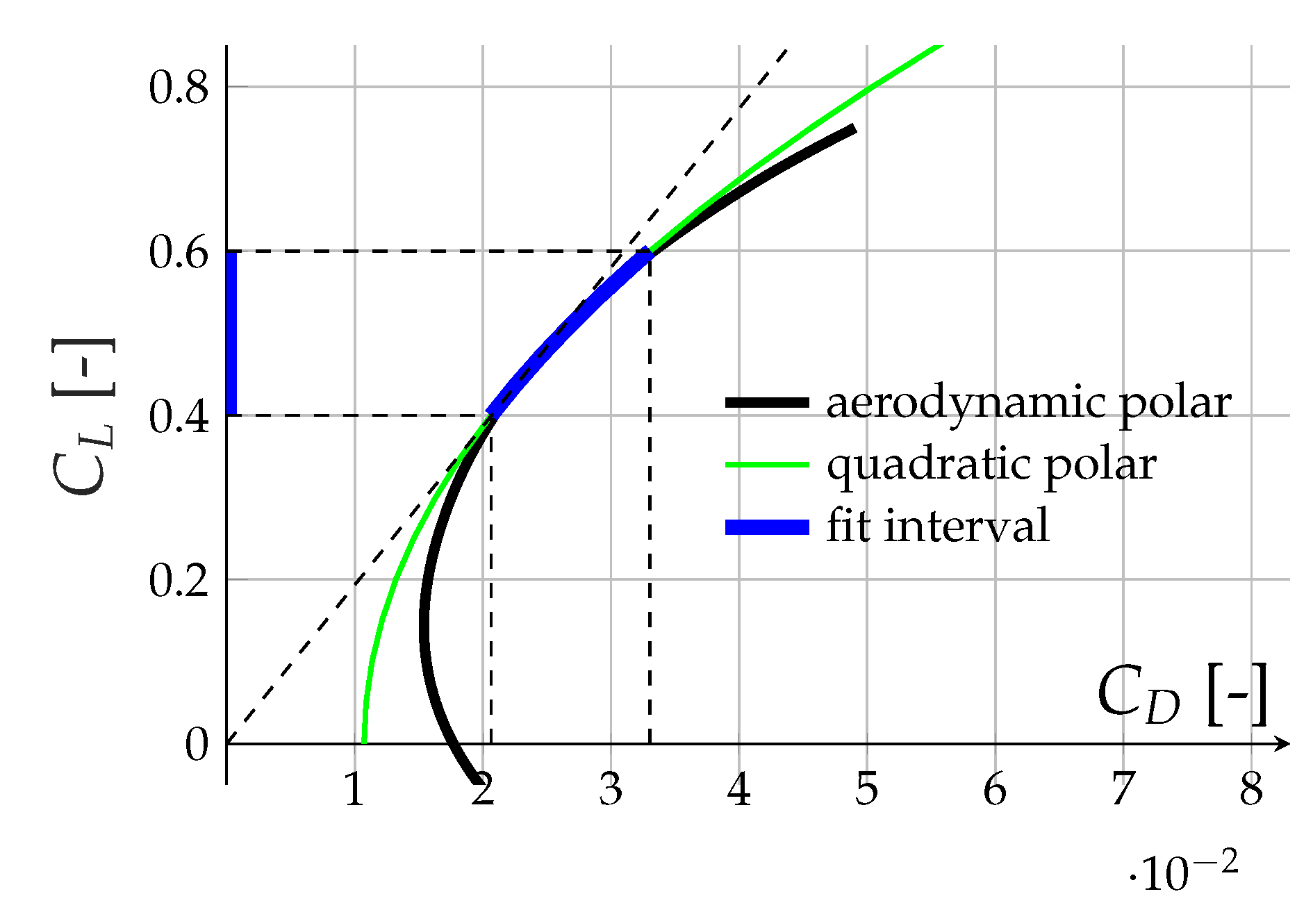
2. Modelling Aspects

In this section, basic aspects of modelling are introduced. To be able to show mathematical-physical relations, the model is built up as simple as possible. It uses a quadratic polar to determine the aerodynamic forces and fix efficiencies of the propulsion components.
Aerodynamic coefficients are modelled by a quadratic polar, which is shown in Figure 1.
It shows the data of a real polar (black) taken from [14]. For the interval of C L = 0.4 , , 0.6 (this interval includes all lift coefficients in the following investigations, as can be seen later), the original data of the polar can be approximated sufficiently by
C D ( C L ) = C D 0 + k C L 2
with the lift and drag coefficients C L and C D respectively. The lift coefficient for best glide amounts C L , ϵ m i n = 0.4154 and is therefore within the interval of approximation. Lift and Drag itself are calculated with the well known equations
L = C L ρ 2 V 2 S
D = C D ρ 2 V 2 S
with air density ρ , flight speed V and reference wing surface S. Atmospherical data is taken from [15].
The differential equations of motion are implemented by
d ˙ = V cos γ
h ˙ = V sin γ
V ˙ = T D m g sin γ
γ ˙ = L m V g c o s γ V
Here, both lateral coordinates are substituted to the distance d. Furthermore, Equations (4)–(7) include altitude h, flight path angle γ , weight m and gravitational constant g (see also [16,17]). Thrust T provided by the propeller and drag D are assumed to be co-linear with V. Wind is not considered and only straight ahead flight, without turns, is regarded as in [14].
The propulsion components include a propeller, an electric motor, a corresponding inverter and a battery as energy storage system. All components’ efficiencies are assumed to be constant. Thus, total efficiency amounts to:
η tot = η Prop η Mot η Inv
0.70 · 0.94 · 0.98 =
65.8 %
which is also taken approximately for the total efficiency of propulsion components in [11]. The propulsive power P prop and the required electric power P el relate with this total efficiency
P prop = T V = P el η tot = U Bat I Bat η tot
with the the battery current I Bat and the battery voltage U Bat = 358.9 V , which is assumed to be constant over the state of charge here. Solved for I Bat , Equation (11) reads as
I Bat = P prop U Bat η tot = T V U Bat η tot
This equation can be found in, e.g., [11].
In addition, the Peukert effect [9] is considered, due to which the effective capacity of the battery is decreasing with increasing current taken from the battery. Therefore, the effective battery current I Bat , eff increases disproportionate with rising battery current I Bat [5]:
I Bat , eff = I Bat I Bat I Bat , nom e 1
Here, the nominal battery current is represented with I Bat , nom = 20 A . To show the impact of the amount of Peukert exponent, three different values e = [ 1.0 , 1.05 , 1.3 ] are applied in this paper (The authors of [5] consider three different types of batteries with Peukert exponents e = [ 1.005 , 1.05 , 1.3 ] . For typical aircraft applications, Lithium-Ion batteries are used holding a Peukert exponent of 1.05 [5,18]). For a Peukert exponent 1.0 , the battery is ideal [see (13)], while for e > 1.0 , the battery is “realistic”, so called in this paper.

3. The Trajectory Optimization Problem

In this work, a trajectory optimization for the presented model is performed. Therefore, the trajectory optimization problem is defined first and is solved by using the MATLAB-Toolbox FALCON.m.
Main goal of the optimization is to reach the fix goal distance with minimum amount of used capacity Δ Q ( t f ) = Q ( t 0 ) Q ( t f ) of the battery. The optimization problem is defined as follows: Find
min C L ( t ) , P prop ( t ) J = Δ Q ( t f )
with respect to the dynamic constraints
x ˙ = f ( x ( t ) , u ( t ) , p ) ,
The state vector x ( t ) contains the states of motion and the remaining capacity Q ( t ) :
x ( t ) = d ( t ) h ( t ) V ( t ) γ ( t ) Q ( t )
The corresponding state derivatives x ˙ include Equations (4)–(7) and
Q ˙ ( t ) = I Bat , eff ( t )
with Equations (12) and (13). The control vector contains the lift coefficient C L and propulsive power P p r o p from (11):
u ( t ) = C L ( t ) P prop ( t )
Here, maximum propulsion power is constrained by P prop 30 k W and for the lift coefficient values within the interval C L = [ 0.3 , 0.8 ] are allowed. The two parameters are final time t f , which is variable in the trajectory optimization, and the Peukert exponent e:
u ( t ) = t f e
In addition, the initial conditions
d ( t 0 ) = 0 m h ( t 0 ) = 500 m V ( t 0 ) = 46 m / s Q ( t 0 ) = 432000 C
the final conditions
d ( t f ) = 70 k m h ( t f ) = 500 m V ( t f ) = 46 m / s
have to be fulfilled ( h ( t 0 ) , h ( t f ) , V ( t 0 ) and V ( t f ) are assumed to be typical values after lift off and before touch down for the described model).
Like in [14], trajectories are optimized using the MATLAB toolbox FALCON.m [19]. With this toolbox, the trajectory optimization problem is defined programmatically. Afterwards, the trajectory optimization problem is converted automatically to a classical parameter optimization problem by time discretization, specifically using trapezoidal collocation. The resulting parameter optimization problem is passed to IPOPT (Interior Point OPTimizer) [20], which solves the problem numerically and returns the result to FALCON.m back again. FALCON.m (FSD OptimAL CONtrol Toolbox for MATLAB) helps to solve the trajectory optimization problem very efficiently by converting the model functions to so called mex-functions [21].

4. Results

In this section, first the optimized trajectories are presented. Afterwards, the altitude dependency due to the Peukert effect is shown and discussed. To conclude, the consumption characteristic of the simplified model is illustrated. With this, the special form of the trajectories and the altitude dependency due to Peukert effect can be explained.

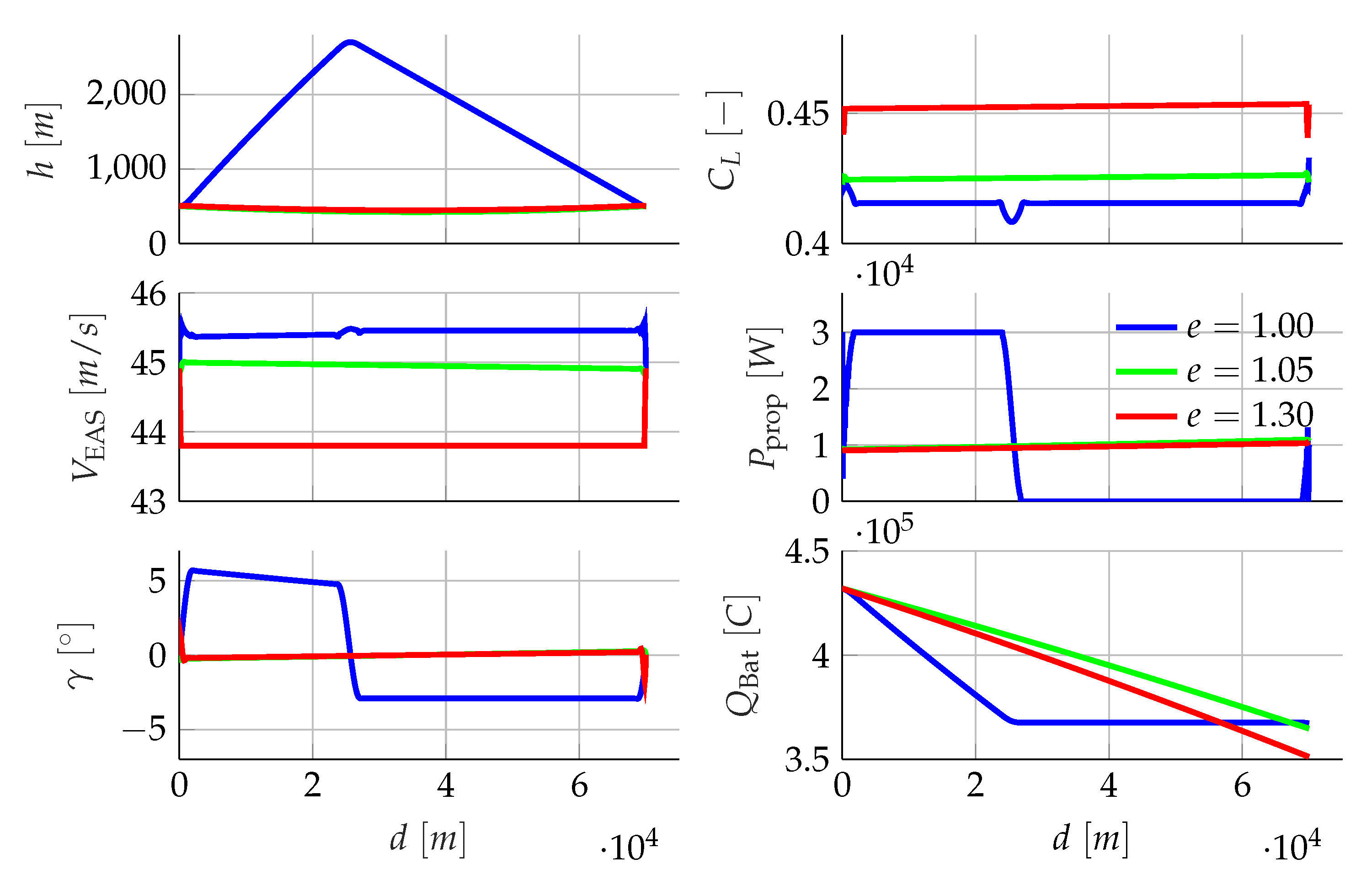
4.1. Optimal Trajectories

Figure 2 shows the resulting optimized trajectories for the three variants of e = [ 1.00 , 1.05 , 1.30 ] (The legend in subplot P prop ( d ) is to be applied to all subplots).
The sub figures depict the histories of the states x and the controls u plotted over the travelled distance d. Here, the velocity V is substituted by the airspeed V EAS = V ρ ( h ) ρ 0 representing the Equivalent Airspeed (EAS), which is corrected for the air density depending on the actual altitude ρ ( h ) .
It can be seen immediately that the form of the trajectory of e = 1.00 differs fundamentally from the two others (The transition phase in the optimal trajectory for the ideal battery is not considered more closely in this paper). While the trajectory e = 1.00 (ideal battery) contains two significantly different segments (climb and glide segment), trajectories with e > 1.00 proceed nearly linear in every diagram. The altitude h and the flight path angle γ represent the progress of the different trajectories: For the ideal battery the climb segment takes a positive (slightly decreasing with rising altitude) γ 5 and a constant negative γ = 3 . In contrast, the histories for the realistic model ( e > 1.00 ) are nearly constant γ = 0 , but both trajectories show a light sink in the altitude progression at about d = 35 k m .
For the ideal battery, the two arcs of the trajectory hold two nearly identical airspeeds, where climb segment airspeed is little smaller than glide segment airspeed. Basically for the realistic model, the airspeed is smaller for bigger values of the Peukert exponent e. This dependency between Peukert exponent and optimal airspeed is presented in [7,8]. Airspeeds for the realistic model are nearly constant over travelled distance d. As all three trajectories are at a quasi steady-state for most of the history, respective airspeeds require different lift coefficients C L . Therefore, a high airspeed (ideal battery; blue) leads to a small C L , while a small airspeed ( e = 1.30 ; red) leads to a big C L [cf. (2)].
The histories of the propulsion power P prop correlate with the trajectories: for the ideal battery, the climb segment takes maximum possible power P prop = 30 k W , while the glide segment does not take propulsion power. Therefore, the glide segment is a pure glide. For the realistic models, the propulsion power is nearly constant. The propulsion power solely increases a little during its history, caused by the little sink in altitude at about d = 35 k m . In the second half of the trajectory, the altitude increases after this sink and a little more propulsion power is required.
This all leads to three different histories of the battery capacity Q ( t ) . Regarding the propulsion power history for the ideal battery, it is obvious that history of battery capacity decreases linearly in the first segment and is constant in the second segment. Because of the quasi linear history of propulsion power for the realistic model, the battery capacity decreases quasi linearly—a little bit steeper for e = 1.30 than for e = 1.05 . The trajectory for e = 1.30 ends with the least remaining battery capacity, while for the ideal battery, it ends with the highest remaining capacity. Obviously, a small Peukert exponent is preferred for less capacity consumption.
Table 1 contains some values gathered from the three trajectories (cf. Figure 2) to give a quantitative comparison. As can be seen in the trajectories, the ideal battery ( e = 1.00 ) consumes the fewest capacity Δ Q . The trajectory for e = 1.05 needs 3.9 % more capacity than the ideal model and the trajectory for e = 1.30 needs 24.8 % . The airspeed for e = 1.05 is only about 0.5 m / s slower in comparison to the ideal model, while for e = 1.30 the airspeed is 1.7 m / s slower. The propulsion power P prop for e = 1.05 and e = 1.30 are nearly equal. Therefore, the battery current I Bat (not I Bat , eff !) is nearly the same for both (not listed in Table 1). However, the effective battery current I Bat , eff for e = 1.30 is over 5 A higher due to the bigger Peukert exponent and (13).
The fastest trajectory reaching d ( t f ) = 70 k m is the ideal model. Despite the longer distance (due to the two segments), it is faster due to its highest airspeed and its progress in higher altitude with less air density additionally. The two other trajectories need more time to reach the goal, due to their slower airspeed V EAS in comparison to the ideal model. Furthermore, the number of iterations and the trajectory optimizations take is different for the three model variants. The trajectory for the ideal model converges remarkably slower than the two remaining trajectories. As shown later, the choice of the altitude does not influence the optimality of the trajectory for the ideal model. The flat gradient causes therefore greater numbers of iterations.

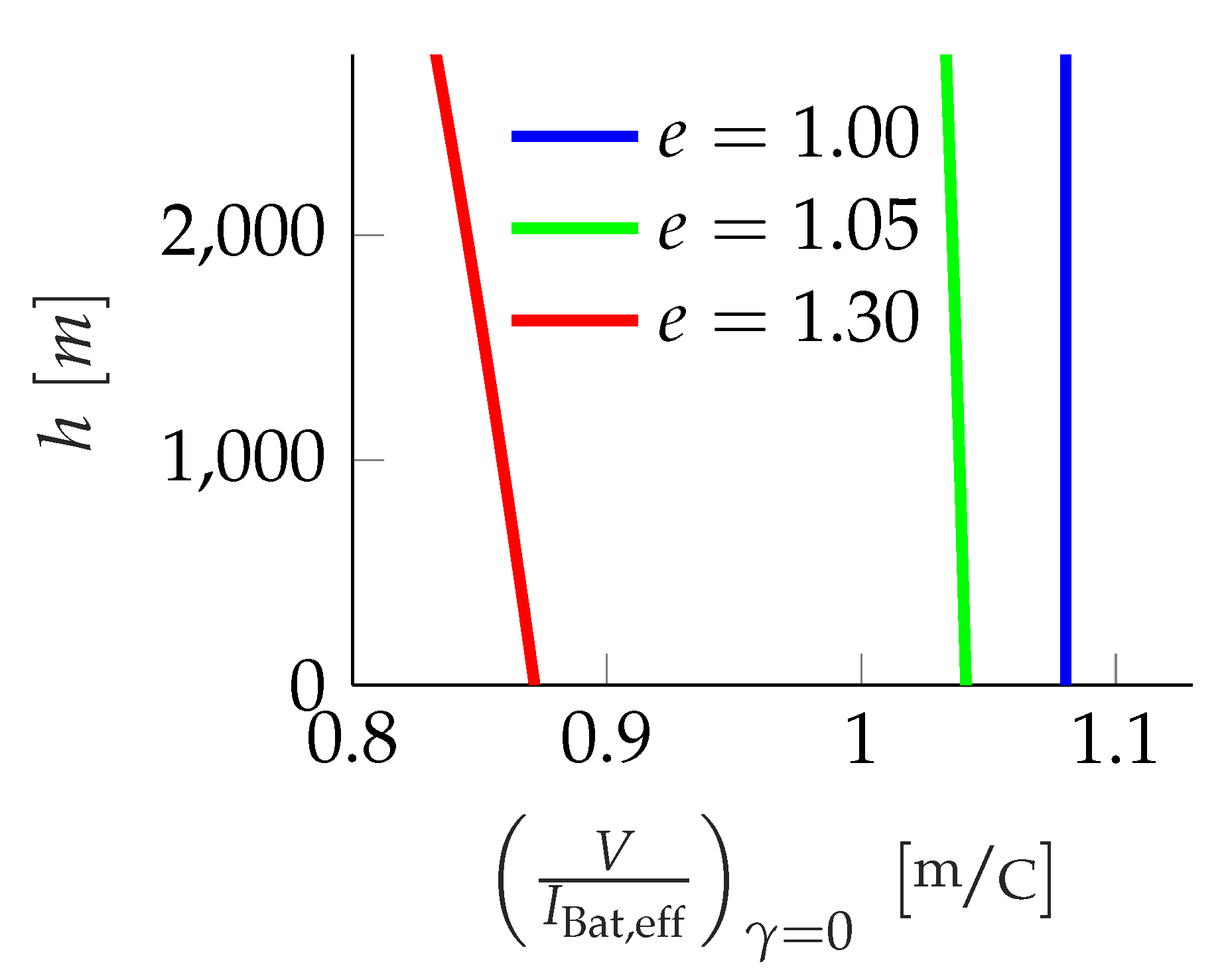
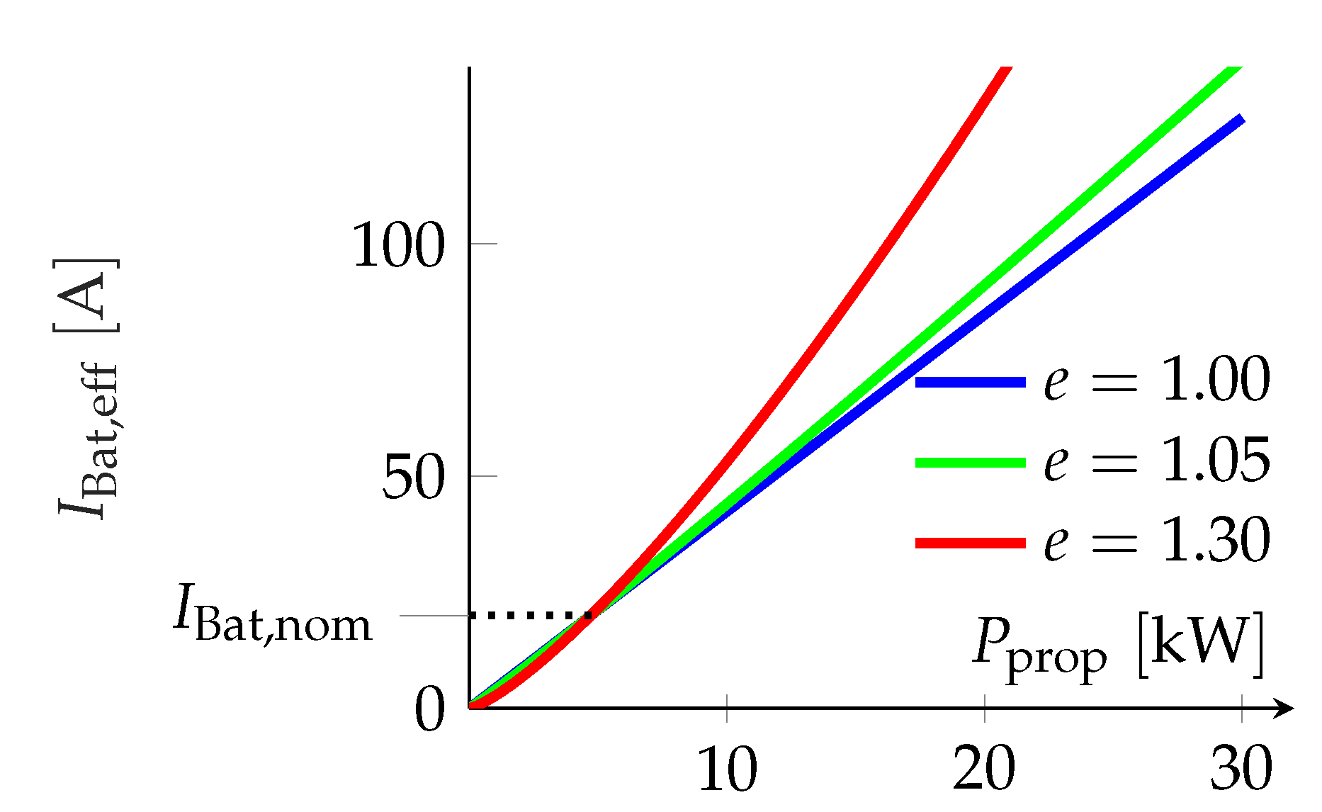
4.2. Steady-State Evaluation

For the evaluation of optimal steady state horizontal flight, the criterion of range optimal flight from [13,14,22] is taken into account. To gain the longest possible travelled distance per amount of capacity, expression
max J = Δ d Δ Q γ = 0
with constant airspeed is to be maximized. For a small d t and with (17), the criterion reads:
max d d t d d t Δ d Δ Q γ = 0 = max V I eff , Bat γ = 0
The equilibrium of forces of a non accelerated ( V ˙ = 0 ) horizontal flight are
L = m g T = D
Therefore, a fix relation between flown airspeed and the lift coefficient is given:
C L ( V ) = 2 m g ρ V 2 S
With the polar (1) the drag coefficient C D is known:
C D ( V ) = C D 0 + 4 m 2 g 2 k ρ 2 V 4 S 2
This leads to the amount of drag in the horizontal flight:
D ( V ) = 1 2 ρ V 2 S C D 0 + 4 m 2 g 2 k ρ 2 V 4 S 2
With Equations (12), (24) and (13), criterion (23) reads as
J ( V ) = V I Bat , nom C D 0 ρ 2 V 4 S 2 + 4 m 2 g 2 k 2 I Bat , nom U Bat ρ V S η tot e
The optimal airspeed to gain maximum range—the Peukert effect taken into account—is presented in [8]. Here, optimal airspeed for maximum range for a quadratic polar is described with:
V opt = 4 m 2 g 2 k C D 0 ρ 2 S 2 · ( e + 1 ) ( 3 e 1 ) 4 = 2 m g ρ S C D 0 k ( e + 1 ) ( 3 e 1 )
(The optimal airspeed can also be derived by analytical study of (28) by zeroing the differential J V , similarly to [7,8].)
Combining (29) and (28), the criterion for optimal range reads as:
J ( V opt ) = V opt I Bat , nom 4 m 2 g 2 k 1 + e + 1 3 e 1 2 I Bat , nom S U Bat η tot ρ V opt e
It can be shown that for the ideal model ( e = 1.00 ) the criterion (30) with optimal airspeed V opt simplifies to
J ( e = 1.00 ) = U Bat η tot 2 m g C D 0 k
and therefore does not contain the air density ρ any more. In other words, the altitude h has no influence considering a range optimal flight of the ideal model ( e = 1.00 ).
For the two other realistic model variants, the criterion (30) contains the air density ρ . Hence, the altitude h has an influence on the criterion’s value. Numerical values of this formula are visualized in Figure 3.
Here, the ideal model ( e = 1.00 ) achieves the maximum possible values and the values are constant over altitude h. The criterion’s values of both realistic model variants are located below. Besides, these values decrease with increasing altitude for e = 1.05 only slightly (≈ 1 % ), and for e = 1.30 significantly ( 5 % ). The smaller the Peukert exponent is, the bigger the maximum reachable range. In addition, flight is more range efficient for the realistic battery models if performed in lower altitudes.
The progressions of the altitude dependency of the realistic models ( e > 1.00 ) are the cause for the form of the optimal trajectories (cf. Figure 2). A trajectory (for the realistic model) in lower altitude is more efficient than in higher altitudes and therefore it proceeds at lower altitudes.

5. Discussion

The form of the optimal trajectories and the altitude dependency of the two realistic models can be explained with the consumption characteristic of the battery-electric propulsion.
Equations (12) and (13) combined show the relation between propulsive power P prop and the effective battery current I Bat , eff :
I Bat , eff ( P prop ) = I Bat , nom P prop I Bat , nom U Bat η tot e
In Figure 4 the consumption characteristics of the three model variants are shown for e = [ 1.00 , 1.5 , 1.30 ] .
The effective battery current I Bat , eff represents the consumption equivalent depending on the propulsion power P prop , as with (17) the effective battery current decreases the available battery capacity Q. The ideal model ( e = 1.00 ) performs exactly linear dependence between propulsive power and effective battery current. For every power taken from the battery the efficiency is equal. Both realistic models show progressions in form of a power function with positive real exponent >1. Above nominal current I Bat , nom , consumption equivalent increases disadvantageously with increasing power for the realistic model in comparison to the ideal model. The bigger the Peukert exponent, the worse the impact is. Below the nominal current I Bat , nom , this phenomenon performs vice versa and therefore a big Peukert exponent is advantageous.
Basically, it is more efficient to avoid huge battery discharge currents over the nominal current to minimize waste of capacity. This explains the altitude dependency as well as the form of the optimal trajectories. The higher the altitude, the less the air density is. To gather the same dynamic pressure ρ 2 V like in lower altitude, airspeed V must be faster in higher altitudes. With (11), more propulsive power is needed. As a consequence of the consumption characteristic of the battery electrical propulsion, the power drain is less efficient at higher power and current, respectively. Thus, higher altitudes are less efficient than lower altitudes in battery-electrically propulsed flight.
This characteristic also influences the form of optimal trajectories. To save capacity, the trajectory for the realistic models proceeds preferably without power-requiring climb segments. Here, the altitude history is as flat as possible. Without the dependency from the air density ρ described above, optimal trajectories would proceed exactly linearly between start and finish.

6. Conclusions

In this paper, impacts of the Peukert effect on optimal guidance of battery electric aircraft are discussed. For this investigation, a variable mathematical model is built up. One model represents an ideal battery with e = 1 , two others (realistic models) take a Peukert exponent of e > 1 into account. Optimal trajectories are generated using those three model variants. Especially the form of the altitude history for the ideal and realistic model diverges. While the ideal model performs a significant climb and glide phase, the realistic models show nearly linear histories between start and goal.
Furthermore, the analysis of an efficiency criterion of range optimal horizontal flight proves that efficiency of a range optimal horizontal flight depends on the altitude. Here, the maximum range with the realistic model can be reached travelling at lower altitudes. The special form of the optimal trajectories, as well as the altitude dependency of range optimal horizontal flight, can be explained with the consumption characteristic of the battery-electric propulsion. For the realistic model, consumption increases disproportionately with increasing battery current (or battery power) in form of a power function with a positive real exponent. The described phenomena are (excepting the altitude histories) bigger, the bigger the Peukert exponent is.
Summarizing, the two main impacts of Peukert effect on optimal flight guidance can be noticed: high discharge currents during flight should be avoided. Therefore, capacity optimized trajectories progress flat and quasi linear on the one hand. On the other hand, range optimal flight should be performed in lower altitudes. These statements are only valid for the described model. If an additional constant discharge current is added to the propulsive power current, results will appear differently. Furthermore, other physical effects placed in the battery (like internal resistance, temperature dependency, inner battery dynamics, etc.) can modify the characteristics. Regarding future battery systems, specific values of the Peukert exponent must be considered for flight performance analysis and assessed taking the field of application of the vehicle into account.

Author Contributions

Conceptualization, F.S., A.K. and F.H.; methodology, F.S., A.K. and F.H.; validation, F.S.; investigation, F.S.; resources, F.H. and A.K.; writing–original draft preparation, F.S.; writing–review and editing, F.H. and A.K.; visualization, F.S.; supervision, F.H. and A.K.; project administration, F.S. and A.K.; funding acquisition, F.S. and A.K.; All authors have read and agreed to the published version of the manuscript.

Funding

This work has been supported by Bayerisches Staatsministerium FÜr Wirtschaft und Medien, Energie und Technologie.

Conflicts of Interest

The authors declare no conflict of interest. The funders had no role in the design of the study; in the collection, analyses, or interpretation of data; in the writing of the manuscript, or in the decision to publish the results.

Abbreviations

The following abbreviations are used in this manuscript:
SymbolsIndices
˙ Time derivative of □[⋯]0zero
C Coefficient of □[−] Bat Battery
DDrag[N] EAS Equivalent Airspeed
dDistance[m] eff effective
ePeukert exponent[−] el electrical
gGravitational acceleration[m/s2]ffinal
hAltitude[m] Inv Inverter
ICurrent[A] Mot Motor
JCriterion[C/s2] min minimum
kaerodynamical Constant[−] nom nominal
LLift[N] opt optimal
mMass[kg] Prop Propeller
PPower[W] prop propulsive
p Parameter vector[⋯] tot total
QCapacity[C]
SSurface[m2]
TThrust[N]
tTime[s]
UVoltage[V]
u Control vector[⋯]
VVelocity[m/s]
x State vector[⋯]
γ Flight path angle[ ]
η Efficiency[−]
ϵ glide path angle[ ]
ρ Air density[kg/m3]

References

  1. Sachs, G. Flight Performance Issues of Electric Aircraft. In Proceedings of the AIAA Atmospheric Flight Mechanics Conference; American Institute of Aeronautics and Astronautics (AIAA), Minneapolis, MN, USA, 13–16 August 2012. [Google Scholar]
  2. Sachs, G. Unique Range Performance Properties of Electric Aircraft. In Proceedings of the AIAA Atmospheric Flight Mechanics (AFM) Conference, American Institute of Aeronautics and Astronautics, Boston, MA, USA, 19–22 August 2013. [Google Scholar]
  3. Traub, L.W. Range and endurance estimates for battery-powered aircraft. J. Aircr. 2011, 48, 703–707. [Google Scholar] [CrossRef]
  4. Hepperle, M. Electric Flight – Potential and Limitations. 2012. Available online: http://www.elib.dlr.de (accessed on 16 August 2017).
  5. Donateo, T.; Ficarella, A.; Spedicato, L.; Arista, A.; Ferraro, M. A new approach to calculating endurance in electric flight and comparing fuel cells and batteries. Appl. Energy 2017, 187, 807–819. [Google Scholar] [CrossRef]
  6. Traub, L.W. Validation of endurance estimates for battery powered UAVs. Aeronaut. J. 2013, 117, 1155–1166. [Google Scholar] [CrossRef]
  7. Avanzini, G.; Giulietti, F. Maximum range for battery-powered aircraft. J. Aircr. 2013, 50, 304–307. [Google Scholar] [CrossRef]
  8. Avanzini, G.; de Angelis, E.L.; Giulietti, F. Optimal performance and sizing of a battery-powered aircraft. Aerosp. Sci. Technol. 2016, 59, 132–144. [Google Scholar] [CrossRef]
  9. Peukert, W. Über die Abhängigkeit der Kapazität von der Entladestromstärke bei Bleiakkumulatoren. Elektrotechnische Zeitschrift 1897, 20, 20–21. [Google Scholar]
  10. Barufaldi, G.; Morales, M.; Silva, R.G. Energy Optimal Climb Performance of Electric Aircraft. In Proceedings of the AIAA Scitech 2019 Forum, San Diego, CA, USA, 7–11 January 2019; p. 0830. [Google Scholar]
  11. Kaptsov, M.; Rodrigues, L. Electric aircraft flight management systems: Economy mode and maximum endurance. J. Guid. Control Dyn. 2017, 41, 288–293. [Google Scholar] [CrossRef]
  12. Falck, R.D.; Chin, J.; Schnulo, S.L.; Burt, J.M.; Gray, J.S. Trajectory Optimization of Electric Aircraft Subject to Subsystem Thermal Constraints. In Proceedings of the 18th AIAA/ISSMO Multidisciplinary Analysis and Optimization Conference, Denver, CO, USA, 5–9 June 2017; p. 4002. [Google Scholar]
  13. Settele, F.; Bittner, M. Energieoptimale Trajektorien für ein batterie-elektrisches Flugzeug. In Deutscher Luft- und Raumfahrtkongress; Hochschule München, Deutsche Gesellschaft für Luft-und Raumfahrt-Lilienthal-Oberth eV: Garching, Germany, 2017. [Google Scholar]
  14. Settele, F.; Bittner, M. Energy-optimal guidance of a battery-electrically driven airplane. CEAS Aeronaut. J. 2020, 11, 111–124. [Google Scholar] [CrossRef] [Green Version]
  15. NASA (Ed.) U.S. Standard Atmosphere; National Aeronautics and Space Administration: Washington, DC, USA, 1976.
  16. Sachs, G.; Lenz, J.; Holzapfel, F. Unlimited endurance performance of solar UAVs with minimal or zero electric energy storage. In Proceedings of the AIAA Guidance, Navigation, and Control Conference. American Institute of Aeronautics and Astronautics (AIAA), Chigao, IL, USA, 10–13 August 2009; pp. 10–13. [Google Scholar]
  17. Menon, P.K.; Sweriduk, G.D.; Bowers, A.H. Study of near-optimal endurance-maximizing periodic cruise trajectories. J. Aircr. 2007, 44, 393–398. [Google Scholar] [CrossRef] [Green Version]
  18. Sun, Y.H.; Jou, H.L.; Wu, J.C. Multilevel Peukert equations based residual capacity estimation method for lead-acid battery. In Proceedings of the IEEE International Conference on Sustainable Energy Technologies (ICSET 2008), Singapore, 24–27 November 2008; pp. 101–105. [Google Scholar]
  19. Rieck, M.; Bittner, M.; Grüter, B.; Diepolder, J. FALCON.m: User Guide; Version 1.14; Technische Universität München: Garching, Germany, 2016. [Google Scholar]
  20. Waechter, A.; Laird, C.; Margot, F.; Kawajir, Y. Introduction to IPOPT: A tutorial for downloading, installing, and using IPOPT. Revision 2009. [Google Scholar]
  21. MathWorks. mex—Build MEX function or engine application. Matlab Documentation. Mathworks, Natick, Massachusetts. Available online: https://de.mathworks.com/help/matlab/ref/mex.html (accessed on 20 November 2019).
  22. Settele, F.; Knoll, A. Grundlagen der Flugführung beim elektrisch angetriebenen Forschungsflugzeug EUROPAS. In Deutscher Luft- und Raumfahrtkongress; Hochschule München, Deutsche Gesellschaft für Luft-und Raumfahrt-Lilienthal-Oberth eV: Augsburg, Germany, 2014. [Google Scholar]
Figure 1. Quadratic Polar.
Aerospace 07 00013 g001
Figure 2. Optimal Trajectories for e = [ 1.00 , 1.05 , 1.30 ] .
Aerospace 07 00013 g002
Figure 3. Values of the criterion for range optimal horizontal flight depicted over altitude h for e = [ 1.00 , 1.05 , 1.30 ] .
Aerospace 07 00013 g003
Figure 4. Consumption Characteristics for e = [ 1.00 , 1.05 , 1.30 ] .
Aerospace 07 00013 g004
Table 1. Quantitative Comparison of Values in the three Trajectories.
e =
1.001.051.30
climbglide
Δ Q [ e 5 C ] 0.648 0.0 0.673 0.809
V EAS [ M M m / s ] 45.4 45.5 45.0 43.8
P prop [ k W ] 300≈10.0≈9.9
I Bat , eff [ A ] ≈1470≈44.2≈50.8
t f [ e 3 s ] 1.422 1.524 1.594
h min [ m ] 420.9 445.2
Iterations [ ] 2743453

