Article

A Simulation-Based Performance Analysis Tool for Aircraft Design Workflows

by
Agostino De Marco
1,*,†,
Vittorio Trifari
2,†,
Fabrizio Nicolosi
1,† and
Manuela Ruocco
2,†
1
Dipartimento Ingegneria Industriale, Università degli Studi di Napoli Federico II, Via Claudio 21, 80125 Napoli, Italy
2
SmartUp Engineering, 80100 Naples, Italy
*
Author to whom correspondence should be addressed.
These authors contributed equally to this work.
Aerospace 2020, 7(11), 155; https://doi.org/10.3390/aerospace7110155
Submission received: 29 September 2020 / Revised: 23 October 2020 / Accepted: 26 October 2020 / Published: 30 October 2020
(This article belongs to the Special Issue Flight Simulation)

Abstract

:
A simulation-based approach for take-off and landing performance assessments is presented in this work. In the context of aircraft design loops, it provides a detailed and flexible formulation that can be integrated into a wider simulation methodology for a complete commercial aviation mission. As a matter of fact, conceptual and preliminary aircraft design activities require iterative calculations to quickly make performance predictions on a set of possible airplane configurations. The goal is to search for a design that best fits all top level aircraft requirements among the results of a great number of multi-disciplinary analyses, as fast as possible, and with a certain grade of accuracy. Usually, such a task is carried out using statistical or semi-empirical approaches which can give pretty accurate results in no time. However, those prediction methods may be inappropriate when dealing with innovative aircraft configurations or whenever a higher level of accuracy is necessary. Simulation-based design has become crucial to make the overall process affordable and effective in cases where higher fidelity analyses are required. A common example when flight simulations can be effectively used to support a design loop is given by aircraft mission analyses and performance predictions. These usually include take-off, climb, en route, loiter, approach, and landing simulations. This article introduces the mathematical models of aircraft take-off and landing and gives the details of how they are implemented in the software library JPAD. These features are not present in most of the currently available pieces of preliminary aircraft design software and allow one to perform high fidelity, simulation-based take-off and landing analyses within design iterations. Although much more detailed than classical semi-empirical approaches, the presented methodologies require very limited computational effort. An application of the proposed formulations is introduced in the second part of the article. The example considers the Airbus A220-300 as a reference aircraft model and includes complete take-off and landing performance studies, as well as the simulation of both take-off and landing certification noise trajectories.

Graphical Abstract

1. Introduction

Nowadays the commercial transport aircraft market is strongly influenced by three main factors. The first conditioning factor, of which the aviation sector has been well aware for decades, is the need to reduce air transportation’s environmental impact, as shown by the evermore ambitious targets defined by associations like ATAG and IATA or the Clean Sky 2 consortium. The second circumstance, bound to have a disrupting effect on all market assumptions made so far, is related to the COVID-19 outbreak in year 2020, which has caused severe damage to the air passenger transportation industry. In particular, recent forecasts by IATA highlight a worldwide 48 % RPK with respect to 2019 [1]. Possible future market scenarios following the worldwide management of the COVID-19 pandemic have been recently provided by ICAO [2]. According to ICAO, given the originally planned seat capacity, passenger demand could have increased 72 million for 2020, compared to 2019. However, the latest estimates expect the passenger demand to drop from the above baseline by 861 to 1524 million. This demand level would be 789 to 1452 million below the passenger demand of 2019, with the most substantial reductions expected to be in Europe and Asia/Pacific. The third main circumstance to be considered in the future evolution of the aircraft market is related to the need for most of the major airlines to replace several hundred heritage aircraft, especially in the regional aircraft segment from 20 up to 150 seats. These airplanes are currently in service around the world and are now coming to the end of their useful commercial lives.
According to the above-mentioned scenario, the period that lies ahead will be difficult and interesting at the same time for aircraft designers, who must face evermore demanding challenges. Preliminary aircraft design can address all these issues, defining a new frontier of innovation in terms of configurations and technologies suitable for the ever-increasing demand for more green and efficient aircraft. In particular, the regional aircraft market segment is playing an increasingly important role in the evolution of airline operations. For many years, this growth has been faced by a wide adoption of regional jets. Their success can be largely attributed to their popularity with passengers, who prefer them thanks to their comfort and velocity with respect to turboprops. However, despite the regional jets’ success, turboprop engines are 10–30% more efficient than jet engines in cruise conditions, leading to potentially consistent reductions of the amount of fuel used per mission and the amount of pollutant emissions [3,4].
The preliminary design phase of new aircraft models has become very challenging due to evermore demanding requirements. The goal of the first stages of a design loop is to search for the configuration that best fits all requirements, among the results of a great number of multi-disciplinary analyses, as fast as possible, and with a certain grade of accuracy. Often, despite being preliminary design, a higher level of fidelity is required, and in such cases simulation-based design has become crucial to make the overall process affordable and effective. A common example where simulation-based design applies is given by aircraft mission analyses and performance predictions. These usually include take-off, climb, en route, loiter, approach, and landing simulations.
The continuous improvement of computer calculation capabilities over years has allowed for the growth of a large family of software tools dedicated to preliminary aircraft design activities, involving also multi-disciplinary analyses and optimizations [5]. The most popular among such computer programs are listed in the following:
  • Pacelab Suite. A commercial software suite, written in C#, developed by the German company Pace, part of the Italian group TXT E-solutions, Milan Italy [6]. This software has rapidly become a leader on the aircraft preliminary design market due to its user-friendliness and its robust and efficient software architecture. The suite is made up of several interconnected modules, each of which adds very important features to the base version (e.g., on-board systems architecture or detailed cabin layout definition). However, some methodologies and databases lack the required scientific know-how that only research centers or universities can provide.
  • SUAVE. A piece of open-source software, written in Python, developed at the University of Stanford, California, USA [7]. It comes with lots of interesting features, among which is the possibility to analyze unconventional configurations (e.g., blended-wing body) with different levels of fidelity, and there is the possibility to take into account different sources of energy (e.g., solar power). However, it has poor visualization features and no dedicated input files, lowering its user-friendliness.
  • FLIGHT. In development since 2006 at the University of Manchester, UK, by Dr. Antonio Filippone, FLIGHT is state-of-the-art software for the prediction and modeling of fixed wing aircraft performance. Through analyzing the performance of airborne vehicles and any sub-systems, FLIGHT can accurately map aircraft operation under all flight conditions, allowing for numerous logistical variations. A unique benefit of the software is the ability to calculate the impacts of noise and LTO emissions, both within and around an airport [8,9].
  • ADAS. Software for the conceptual/preliminary design of transport aircraft (transport jet, regional turboprops, business jet) and light aircraft developed at the University of Naples Federico II, Naples, Italy, by Fabrizio Nicolosi and Giuseppe Paduano [10]. The software, in development since 2005, is completely written in Visual Basic and comes with a dedicated graphic user interface to enhance user-friendliness. Its architecture provides for independent design modules; however, it was not conceived for MDAO applications.
  • CEASIOM. A conceptual aircraft design framework by CFS Engineering, Lausanne, Switzerland, written in Python, developed within the frame of the SimSAC (Simulating Aircraft Stability And Control Characteristics for Use in Conceptual Design) Specific Targeted Research Project (STREP) approved for funding by the European Commission 6th Framework Programme on Research, Technological Development and Demonstration. CEASIOM is meant to support engineers in the conceptual design process of the aircraft, with emphasis on the improved prediction of stability and control properties achieved by higher-fidelity methods than found in contemporary aircraft design tools. Moreover, CEASIOM integrates into one application the main design disciplines: aerodynamics, structures, and flight dynamics, impacting on the aircraft performance. However, the framework does not carry out the entire conceptual design process; thus, it requires as input an initial layout. as the baseline configuration that it then refines and outputs as the revised layout [11]. For this reason, the framework has been used in combination with the above-mentioned ADAS software [12].
  • Piano. A professional tool by Lissys Limited, UK, for the analysis of commercial aircraft available since 1990. It is used in preliminary design, competitor evaluation, performance studies, environmental emissions assessments, and other developmental tasks by airframe and engine manufacturers, aviation research establishments, and governmental or decision-making institutions throughout the world [13].
  • ADS (Aircraft Design Software). A piece of commercial software developed by OAD (Optimal Aircraft Design), Belgium, after six years of development which has become a standard for the conceptual design of the modern generation of light aircraft. The tool is suitable for several kind of customers, among which are aircraft designers, amateur builders, universities, and research institutes [14].
  • AAA (Advanced Aircraft Analysis). Commercial software developed by DARCorporation, Lawrence, Kansas, USA, and widely used by industries and Universities. The tool is suitable for conceptual and preliminary design phases of both conventional and unconventional fixed wings aircraft configurations. The software allows for multi-fidelity analyses, combining classical and fast semi-empirical methodologies with physics-based methods. In addition, a graphic user interface provides for the required user-friendliness [15].
  • RDSwin. Developed by the design and consulting company founded by Daniel P. Raymer, Conceptual Research Corporation, Playa del Rey, CA, USA, this commercial software was conceived to support industries, governments, and universities during preliminary aircraft design activities. It performs MDAO, as well as trade studies, and comes with a graphic user interface to enhance user-friendliness. The tool is suitable both for commercial transport aircraft and military fighters, giving to users the possibility to experiment also with unconventional configurations [16].
In addition, there are several architectures available nowadays dedicated to the multi-disciplinary design optimization (MDO), most of which were born from the specific needs of aircraft designers. A general survey of such methodologies and their implementations is found in [17], which introduces the well known unified descriptions of MDO architectures and discusses the features of both monolithic and distributed frameworks. A notable example of research effort involving some level of simulation-based performance analysis optimization is given by the work of Kroo from Stanford University [18,19] with his Collaborative Application Framework for Engineering (CAFFE) [20,21]. Martins from the University of Michigan is the leader of a prolific research group (Multidisciplinary Design Optimization Laboratory, MDO Lab) that has released some well known optimization architectures, including the π MDO environment [22], the framework pyOpt [23,24], and the popular optimization software OpenMDAO [25]. Two other interesting works in the MDO field are the Decision Environment for Complex Designs (DECODE) project at the University of Southampton [26], based on the value-driven design concept, and the Chinese research on virtual simulation architectures inspired by the “design for operations” idea [27].
A key feature that most of these pieces of software provide is the possibility to parametrically define both aircraft components and complete aircraft configurations, leading to a very fast and intuitive definition process of a generic aircraft model. One feature missing in most of the above-mentioned tools is the ability to perform simulation-based performance analyses. The goal of this article is to present a mathematical model and its corresponding implementation that fills this gap, and to introduce a piece of software able to perform high fidelity take-off and landing analyses in the context of preliminary design.
The authors of the present article have been users of most of the above-mentioned computer programs, and they have reached a mature vision of the set of features one must expect from a modern MDAO software. This vision drove the development, started in 2015, of a modular framework named JPAD (Java API for Aircraft Designers) that gathers all the lessons learned in the last few decades of in-house tool development for aircraft design [28]. JPAD is an application programming interface (API) able to support civil transport aircraft designers in the need for building multi-disciplinary, simulation-based analysis and optimization workflows. The API is a Java software library containing classes and utility functions that can be used to build software systems running MDAO procedures [5,28,29,30,31,32,33]. JPAD comes in different interdependent software modules providing modeling, simulation, and analysis features. An introduction to the aircraft geometric modeling possibilities provided by JPAD is given by [34]. The API provides a simulation-based aircraft performance module whose implementation details are introduced by this article. An example of application of this feature can be found in [35], where several flight simulations have been used to find trade factors and response surfaces related to environmental noise, DOC, and pollutant emissions for the design of a transport aircraft configuration with rear-mounted engines. As described in [5], JPAD is also provided with an MDAO module which uses all the advantages provided by the Object-Oriented Programming philosophy to perform a full factorial DOE as well as multi-objective optimizations using computational intelligence like GA or PSO algorithms.
This article is organized as follows: Section 2 presents JPAD as a software library and gives an overview of the API as the technological foundation for the aircraft performance model. Section 3 introduces the performance simulation model and provides details of the implementation architecture. Finally, Section 4 presents an application example of the JPAD performance simulation module to the case of a reference regional transport aircraft.

2. Overview of the JPAD Software Library

The API of JPAD defines a unified model of a generic transport aircraft and comes as a software library in different interdependent modules. Rather than being monolithic computer code, this library provides a large collection of modeling, simulation, and analysis capabilities that can be used as building blocks of computational workflows. The modules at the core of the software architecture are shown in Figure 1. This level of modularity gives a unique flexibility to the software framework, which is easily extendable for future market and research challenges.
JPAD has been developed from scratch with the following driving ideas:
  • To provide a modern, user-friendly preliminary aircraft design toolbox;
  • To embed calculation methods with a validated level of accuracy and reliability;
  • To be able to perform multi-disciplinary analyses and optimizations;
  • To provide executables that require reasonably short computational times for a complete aircraft analysis process.
The multi-disciplinary approach in particular, which is very important in the modern software framework nowadays, is summarized in Figure 2. In addition, to ensure longevity and to enrich its applicative scenarios, the library provides multiple fidelity analysis methodologies and is designed to be extended very easily with newly implemented surrogate models. For instance, as discussed in [5,34], JPAD offers the possibility to easily generate and export an aircraft configuration CAD model in one or more standard formats and to execute high-fidelity analyses by means of third-party external tools (e.g., computational fluid dynamics or finite element method solvers). Without these features it would be extremely difficult to achieve an optimum design that reflects the requirements of aircraft performance, noise and emissions levels, and maintenance and operative costs.
In recent years, the development of JPAD has embedded the knowledge and experience gained by the developing team concerning the setup, testing, and validation of several approaches and methodologies related to aircraft design [36,37,38]. The experience includes several research efforts in innovative technologies, such as design campaigns on airfoil and high lift devices, and activities related to performance estimation of aircraft with morphing devices [39,40,41]. Moreover, JPAD incorporates an improved semi-empirical model for vertical tail plane design that was accomplished by means of a campaign of both numerical and experimental studies [33,42,43]. This methodology was also applied to size the vertical tail plane of a new twin-engine commuter aircraft [44]; then its validity was confirmed by wind tunnel tests [45]. Earlier research activities were focused on aerodynamic derivative estimation [46]. Another methodology for fuselage design and prediction of its aerodynamic characteristics based on a surrogate model was developed through CFD-RANS calculations performed on several fuselage geometries suited for regional transport aircraft [47]. Most of this knowledge have been included in the software library using lookup tables packed in dedicated databases [5].
A rather unique capability of JPAD, when compared to other similar software, is that it provides a performance analysis module based on a quite refined set of simulation models. The non-terminal, up-and-away flight phases of a mission are simulated by resolving a set of nonlinear aircraft performance equations (NAPE) adapted from [48]. The terminal flight phases of a mission, such as take-off and landing, have their dedicated models, which are tailored for the designer’s specific needs to assess the compliance of results with regulation requirements. All available models are conveniently coupled to allow the simulation of a full mission with realistic navigation requirements and constraints. The details of take-off and landing simulations models are presented in the following section.

3. A Simulation-Based Approach for Take-Off and Landing Performance Assessment

The performance analysis module in JPAD has been completely designed using a simulation-based approach to carry out both flight and ground performance studies with a high level of fidelity. This feature is usually not implemented inside most of the currently available preliminary aircraft design software, which relies on semi-empirical approaches, especially for the take-off and the landing phases.
The JPAD core library includes simulation procedures that predict aircraft performance figures related to each mission phase. The main mission analysis module features several sub-modules and provides the possibility to perform a single performance analysis (e.g., a detailed take-off, climb, or landing simulation), a complete mission profile analysis, or a combination of them. The user can easily configure which analyses must be carried out using a dedicated XML configuration file (see Figure 2). In terms of software engineering work, particular attention has been paid to the implementation of performance predictions within JPAD, to find the right balance between flexibility, accuracy, computational time, and simulation details. Therefore, although the performance module is the most demanding one in terms of CPU time among all other low and middle fidelity analysis modules available in the library, the possibility for the user to manually enable or disable each sub-analysis enables quite acceptable computational demands for mission assessments.
In the overall JPAD core dependency map, the performance module requires some aircraft weight data as well as trimmed aerodynamic data concerning polar drag curves and lift curves in every standard flight condition (take-off, climb, cruise, and landing). The inputs can be assigned by the user manually—if the analysis is carried out in standalone mode, i.e., when a single focused performance study is required—or they can be fetched from a higher level aircraft analysis manager instance—e.g., when a full-blown design loop is executed. In the first case, two approaches are possible: working with parametrically defined parabolic drag polar curves, or using external drag polar curves if the user has higher fidelity data. In any case, lift curve data must be given using only the following parameters in clean, take-off, and landing configurations: lift curve slope, lift coefficient at zero angle of attack, and maximum lift coefficient. In addition, also the rudder effectiveness coefficient τ r must be specified, in case of a standalone take-off study, to allow the estimation of the minimum control speed ( V MC ). That is the minimum speed for which a sudden, single engine failure (with the remaining engines at take-off power) does not result in loss of primary flight control.
All performance assessment procedures use an engine database for each installed engine (multiple types of engine are possible in order to model hybrid propulsion aircraft). The user also has the possibility to define a wide set of calibration factors (all set to 1.0 by default) to trim all engine related quantities (thrusts, SFC, and emission indexes) for each engine rating (maximum take-off, APR, maximum climb, maximum continuous, maximum cruise, flight idle, and ground idle).
The performance module in JPAD currently features the following analyses:
  • Take-off;
  • Landing;
  • Take-off and landing noise trajectories;
  • Climb;
  • Cruise;
  • Descent;
  • Mission profile;
  • Payload-Range diagram;
  • V-n diagram.
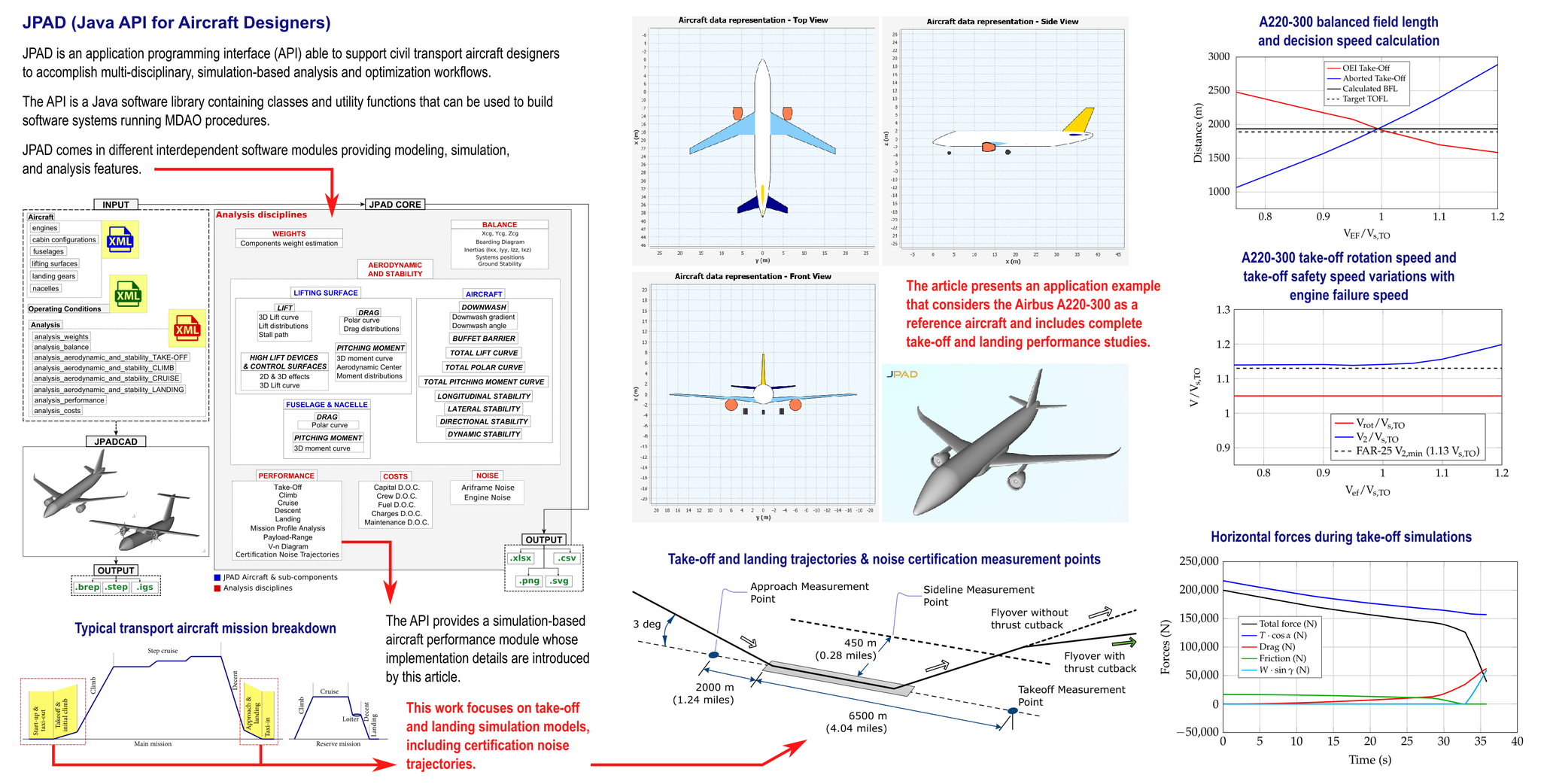
Among them, this section focuses on take-off, landing, and certification noise trajectories analysis modules. A detailed description of the implemented simulation methodologies is provided, which highlights important features usually not considered by classical semi-empirical approaches used for typical preliminary design activities.

3.1. Take-Off Simulation Model

The take-off analysis module computes conventional aircraft take-off performance using a simulation model first proposed in [28]. However, due to major modifications that have been recently implemented, a review of the methodology is presented here.
The analysis procedure solves a set of ODEs that model the aircraft equations of motion during the whole take-off phase, including the ground roll, the transition to the airborne phase, and the initial climb, up to (and beyond) the conventional standard established by regulations. The aircraft is modeled as a point mass constrained to move in a vertical plane under the action of propulsive, aerodynamic ground contact forces and weight, and hence is treated as a dynamic system in its state-space representation. The unknowns are the following fundamental variables of motion that describe completely the aircraft’s state during the whole maneuver:
  • Position s, i.e., center of gravity projected vertically on ground;
  • Ground speed V;
  • Flight path angle γ ;
  • Center of gravity altitude above the ground h;
  • Mass m.
The take-off state equations are then written in the following compact form x ˙ = f ( x , u ) that can be expressed as [28]:
s ˙ V ˙ γ ˙ h ˙ m ˙ = f 1 V f 2 V , γ , h , m ; α f 3 V , γ , h , m ; α f 4 V , γ f 5 V , γ , h with x 1 = s x 2 = V x 3 = γ x 4 = h x 5 = m and u = α
where the unknown x = [ 2 m u x 1 , x 2 , x 3 , x 4 , x 5 2 m u ] T are the vector of state variables, and the input u ( t ) is a given function of time that corresponds to an assumed angle of attack time history during take-off. The right-hand side of system (1) is defined by the following functions:
f 1 V = x 2
f 2 V , γ , h , m ; α = g W T ( x 2 ) D ( x 2 , x 3 , x 4 , x 5 , u ) μ W L ( x 2 , x 3 , x 4 , x 5 , u ) if S ( x 2 , u ) < 1 ( on ground ) T ( x 2 ) cos u W sin x 3 D ( x 2 , x 3 , x 4 , x 5 , u ) if S ( x 2 , u ) 1 ( airborne )
f 3 V , γ , h , m ; α = g W x 2 0 if S ( x 2 , u ) < 1 ( on ground ) L ( x 2 , x 3 , x 4 , x 5 , u ) + T ( x 2 ) sin u W cos x 3 if S ( x 2 , u ) 1 ( airborne )
f 4 V , γ = x 2 sin x 3
f 5 V , γ , h = m ˙ f ( x 2 , x 3 , x 4 )
where T is the total thrust (for all engines set to maximum Take-off rating), D is the aerodynamic drag, L is the aerodynamic lift, W is the weight, and μ ( W L ) is the tangential force proportional to the rolling friction coefficient μ .
Thrust calculations are performed for each engine separately and then summed together to have the total value T. Each thrust vector intensity is calculated by means of a known interpolating function T tab V a based on a table lookup algorithm, where V a = V + V w is the instantaneous airspeed and V w is an assigned constant wind speed (horizontal component, negative in case of headwind). Consequently, the total thrust becomes a function T ( x 2 ) of the ground speed V. The total thrust vector is projected on the aircraft body-fixed reference frame and its components are used appropriately. The mass state function f 5 is given by the the fuel flow m ˙ f , which is calculated by a table lookup interpolating function included in the engine datapack. The drag D and lift L, as functions of airspeed, altitude, flight path angle, aircraft mass, and angle of attack, are given by the following conventional formulas:
D ( x 2 , x 3 , x 4 , x 5 , u ) = 1 2 ρ x 2 + V w 2 S C D x 2 , x 3 , x 4 , x 5 , u
L ( x 2 , x 3 , x 4 , x 5 , u ) = 1 2 ρ x 2 + V w 2 S C L x 2 , x 3 , x 4 , x 5 , u
The switching function S of aircraft velocity and angle of attack is defined as follows:
S ( x 2 , x 3 , x 4 , x 5 , u ) = L ( x 2 , x 3 , x 4 , x 5 , u ) W cos x 3
The lift coefficient C L ( x 2 , x 3 , x 4 , x 5 , u ) is taken from the aircraft trimmed lift curve with high-lift devices (flaps, and slats if present) deflected in take-off positions. The same applies for the drag coefficient C D ( x 2 , x 3 , x 4 , x 5 , u ) . This justifies the dependency of these two aerodynamic coefficients on aircraft mass. Both these coefficients are then scaled to take into account the ground effect on the induced drag, as proposed in [49].
The set of formulas (2) makes (1) a closed system of ODEs. When the function u ( t ) is assigned and the system is associated with a set of initial conditions, in this particular case equal to x 0 = [ 0 , 0 , 0 , 0 , 0 ] T , a well-posed IVP is formed, which can be solved numerically.
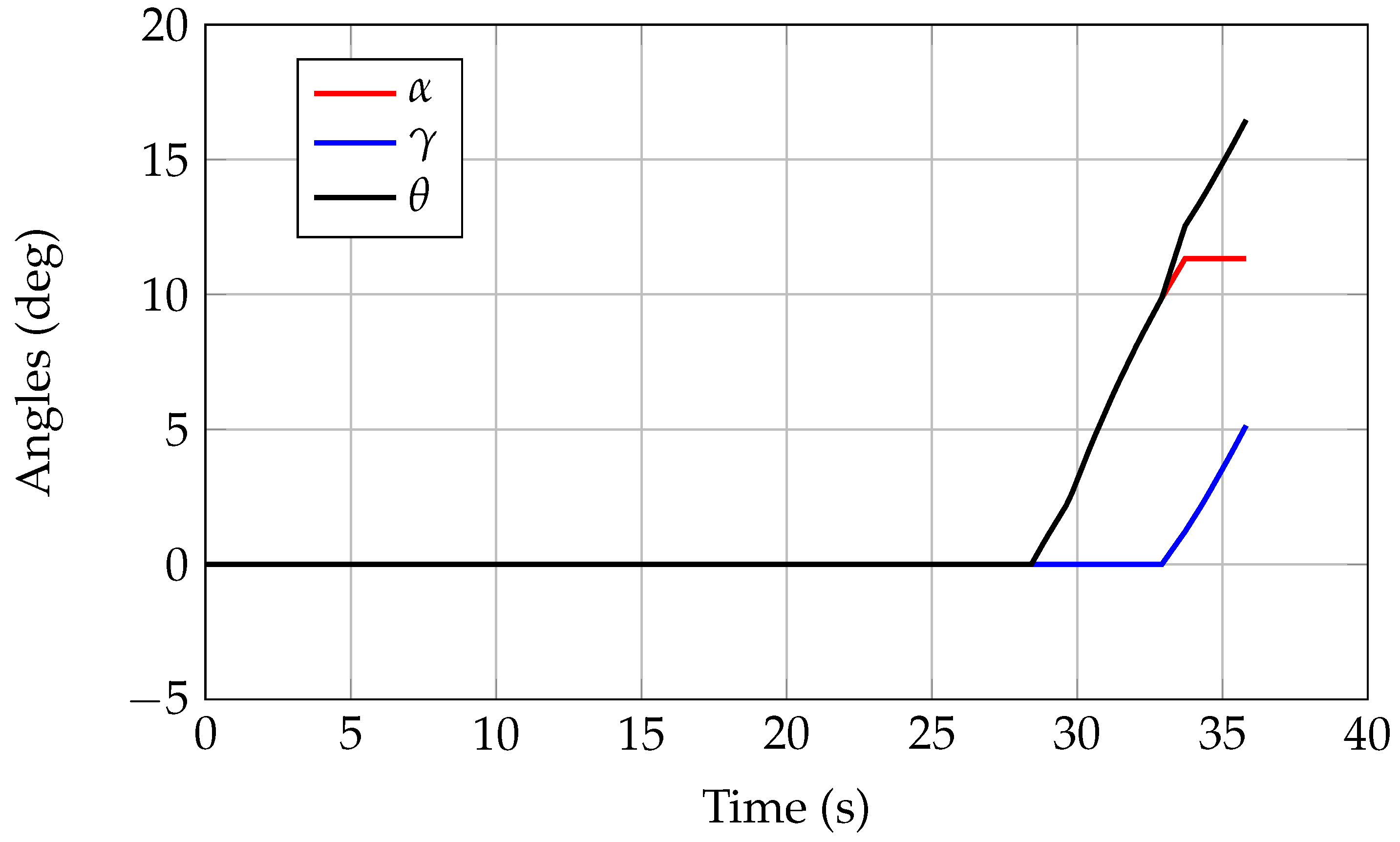
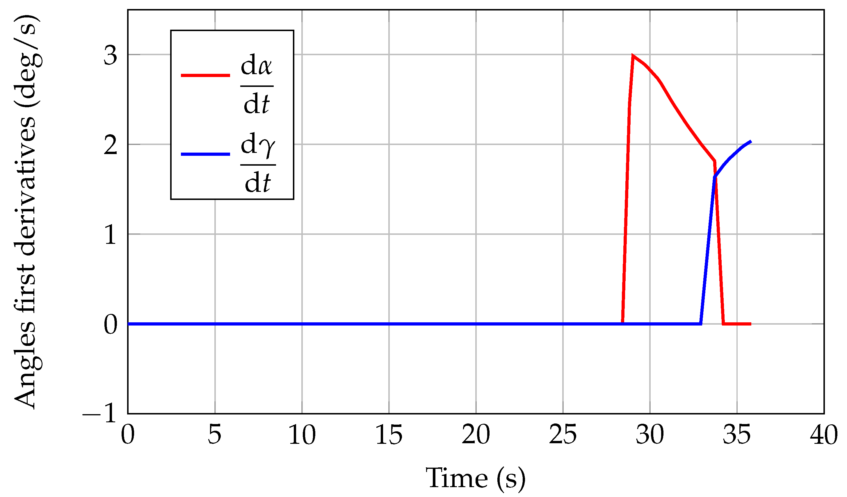
The function of time u ( t ) 
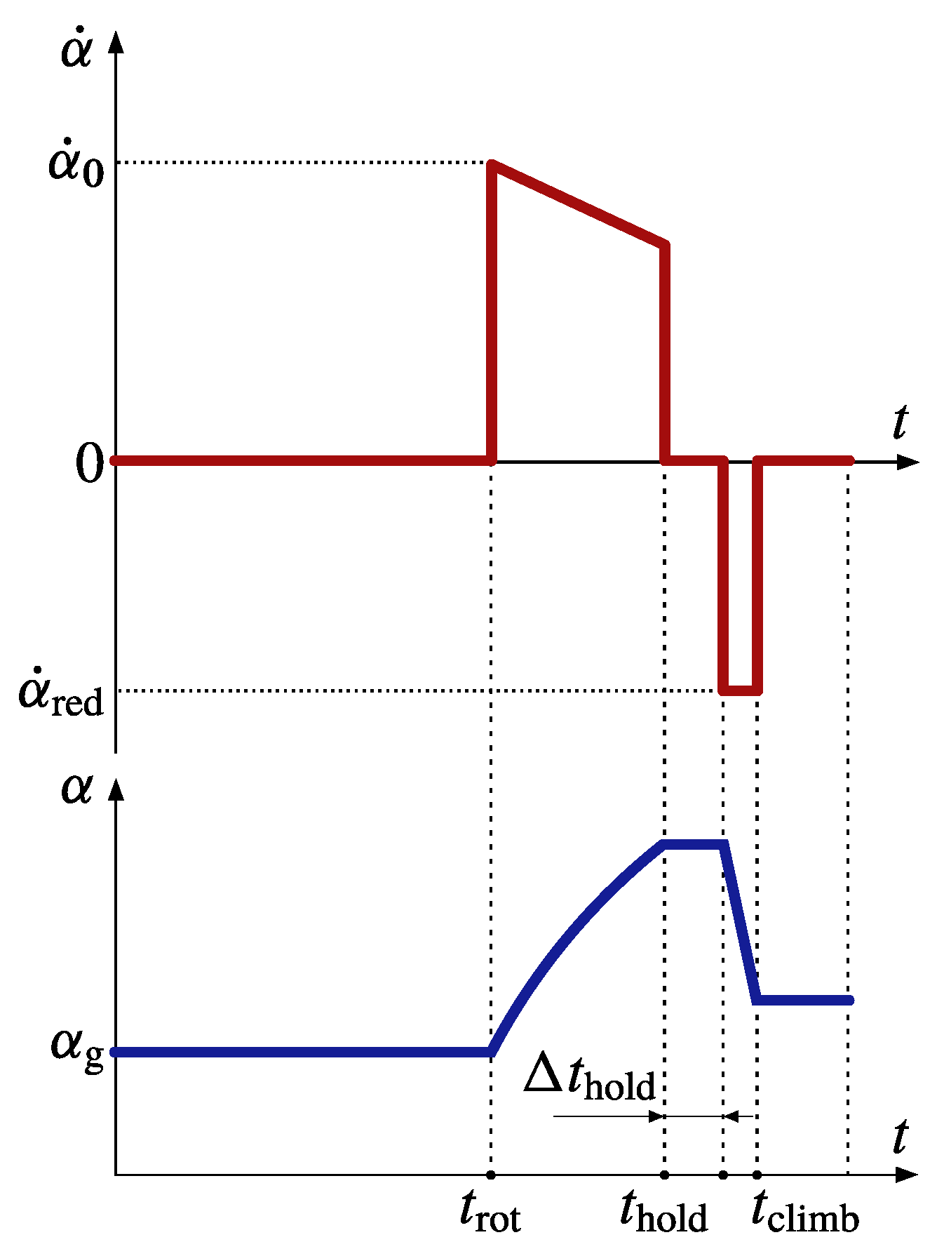
represents the input law of the angle of attack and is defined as follows:
u ( t ) = α g if t < t rot α 1 ( t ) if t t rot
where t rot is the time during the ground roll at which the aircraft rotation starts, that is, when V reaches a given value V rot called rotation speed. The function u ( t ) is represented in Figure 3. In Equation (3), the methodology assumes a constant angle of attack α g during the ground roll phase up to the rotation speed, and a given non-zero law α 1 ( t ) for the post-rotation angle of attack time history. After the rotation, the angle of attack changes according to an assigned initial value of its time derivative α ˙ 0 , which decreases with time according to the following law:
α ˙ = α ˙ 0 1 k α α
that is, as a function of the instantaneous angle of attack, until the time t hold is reached. In this particular instant the aircraft achieves the maximum admissible lift coefficient in take-off configuration, which is set by default at 90% of the maximum achievable take-off lift coefficient. In Equation (4), the slope k α and the initial angle of attack time derivative α ˙ 0 are assigned as inputs. From time t hold onward, the pilot keeps the angle of attack constant for an assigned time interval Δ t hold , during which the airplane decelerates due to a higher induced drag. After this short time interval, the pilot must reduce the angle of attack in order to contain the deceleration. Hence, a negative time derivative α ˙ red is considered after time t hold + Δ t hold 
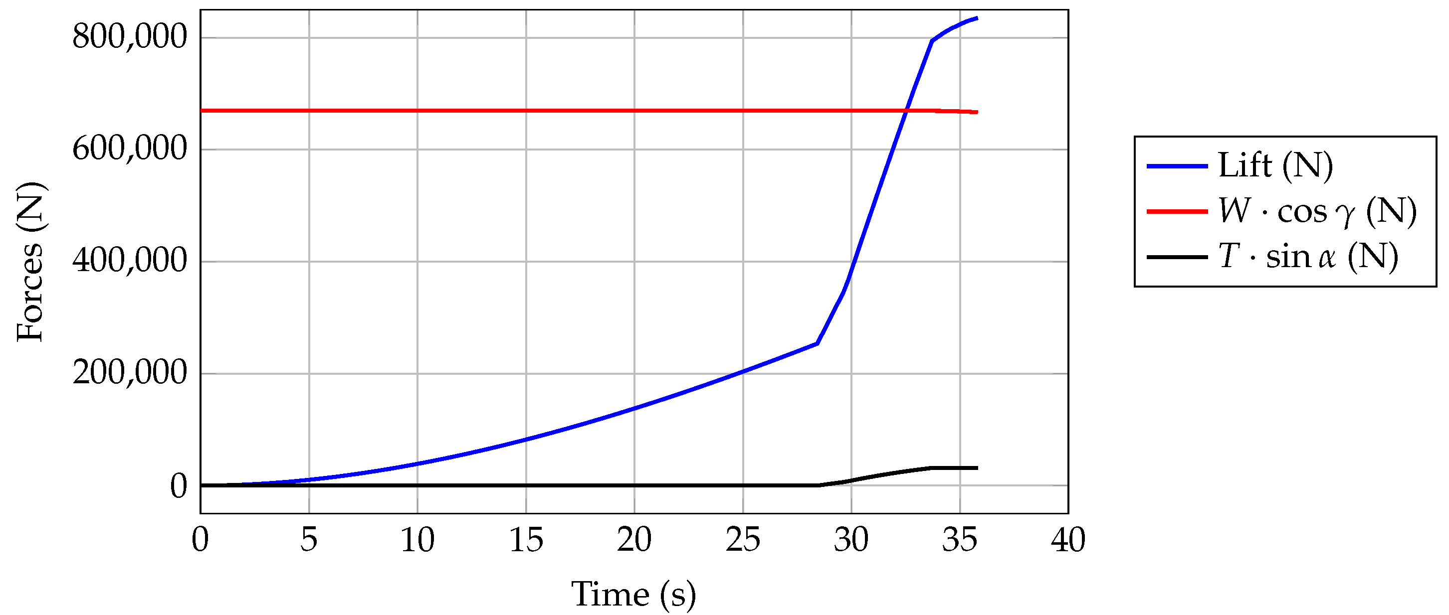
, assumed constant for simplicity. Finally, since the decrease in angle of attack provides also for a reduction in lift coefficient, the time t climb will be reached when the load factor is reduced to a value of 1. This means that a balance of forces perpendicular to the flight path has been achieved and α ˙ returns to a value of 0. The model assumes a steady climbing flight after time t climb .
During the simulation, the fuselage attitude angle θ = γ + α is constantly monitored to ensure the absence of tail strike. If the tail touches the ground a visual warning is launched by the calculation module.
The calculation of take-off distance in OEI condition is quite the same as the nominal AEO case, with the difference being that when one engine becomes inoperative during the maneuver there is a discontinuity in thrust, and a drag increment due to the failed engine [50]. In the event of an engine failure during the take-off ground run, the pilot must decide whether to continue the take-off, or instead, abort the maneuver and decelerate to a stop. Obviously, if the engine failure occurs when the aircraft is traveling very slowly, the aircraft should be kept on the ground and brought to a stop at some safe location off the runway. Conversely, if the engine failure occurs when the aircraft is faster than the decision speed, the take-off should be continued. The designer must provide a means for deciding whether it is safer to reject the take-off or continue the maneuver.
The critical velocity, denoted as V act , is the velocity at which action is done. The time between the recognition of an engine failure, which occurs at V ef , and the critical velocity V act , when action is performed, is required to be more than one second. Generally, this time period, which is set by the reaction time of the average pilot, is taken to be about 1 s ÷ 2 s . If the pilot’s decision is to continue the take-off with one engine inoperative, the distance to the point where lift-off speed V LO is achieved, and to the subsequent climb-out to 35 ft height above the runway, will obviously be longer than the case with all engines operating. The calculation of the take-off distance in this situation is quite the same as the one that determines the nominal take-off length, with the difference being that now there is an abrupt change in total thrust time history. In particular, individual contributions to T ( x 2 ) are still read from the database but considering a number of engines reduced by one from the time t ef at which the engine failure occurred.
On the other hand, in case of rejected take-off, the pilot will apply the necessary braking procedures in order to get the maximum allowed deceleration while maintaining adequate control of the airplane’s motion. From time t ef when the engine failure occurs, i.e., when velocity assumes a value V ef , until the pilot reacts by activating brakes, there is only a discontinuity in thrust. After an assigned time interval in which the pilot decides to abort the take-off, the thrust is set to minimum (ground idle engine rating), brakes are activated, and a higher friction coefficient is set. During this phase, the Equation (2b) changes in the following way:
f 2 x , u = g W D ( x 2 , u ) μ brakes W L ( x 2 , u )
where μ brakes is bigger than μ and it is usually about 0.3 or 0.4.
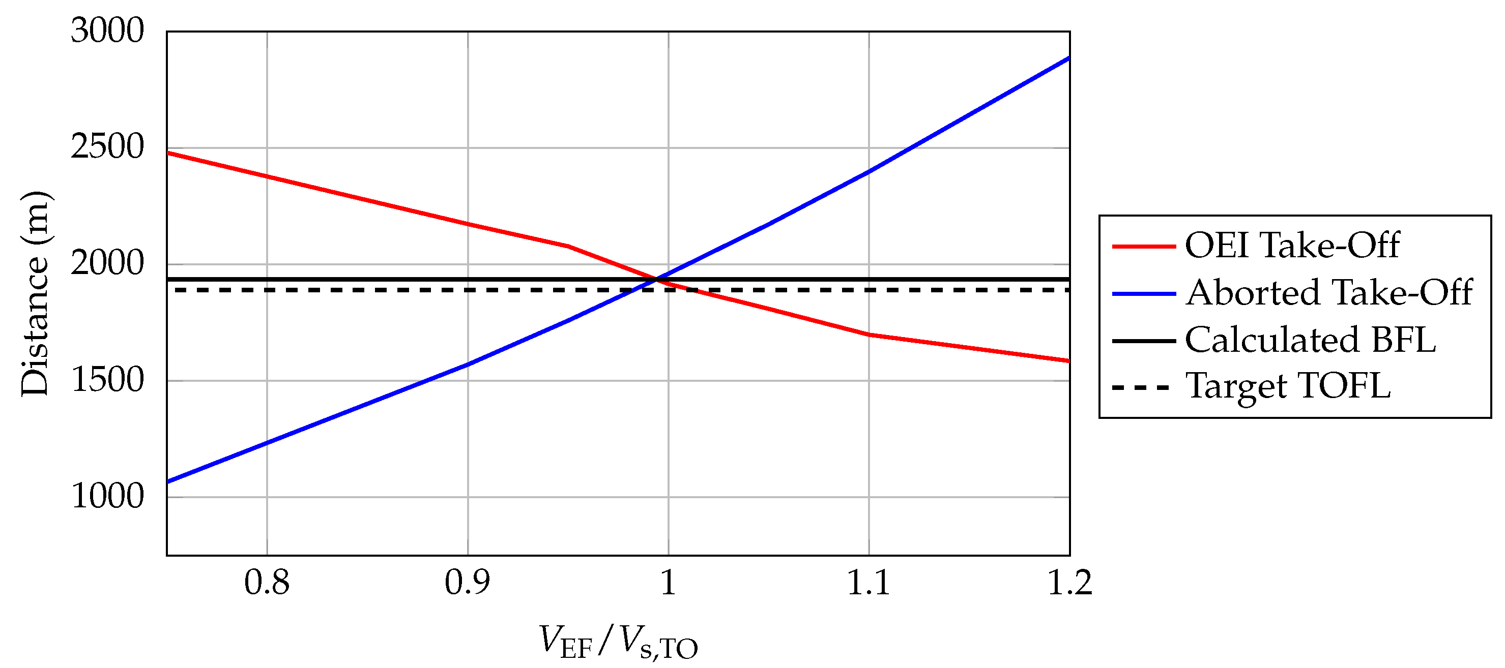
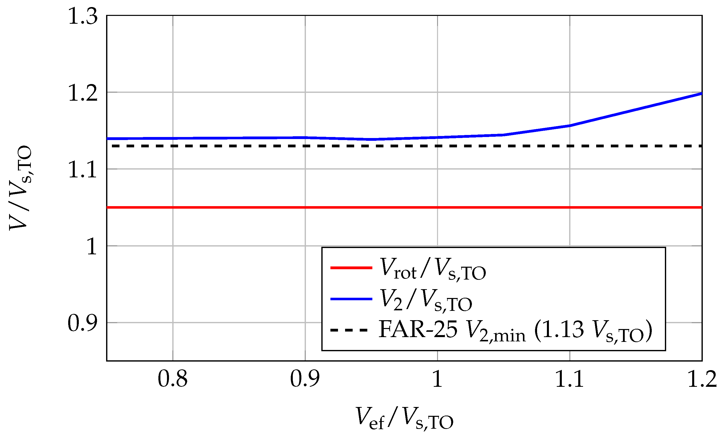
Instead of considering the limiting cases of an aborted take-off at low V act and a OEI take-off at high V act , it is useful to determine the critical velocity at which the distance required to continue the take-off with one engine inoperative equals the distance required to safely abort it. This velocity is the decision speed named V 1 by regulations, while the related distance is the balanced field length, BFL. To calculate this distance and the related velocity, both the OEI take-off distance and the aborted take-off distance are estimated at different V act . These two distances are then plotted against the corresponding engine failure speeds, and the intersection of the two curves, at which the two distances are the same, defines the BFL and the V 1 (see Figure 4).
Although JPAD provides for default values for most of the inputs necessary to perform take-off simulations, the user has the possibility to manually assign each of them. The list of inputs to the take-off analysis module is reported in Table 1. The user can define the desired percentage of the take-off stall speed required to calculate the rotation speed. However, according to FAR regulations [51] (part 25, subpart B, paragraph 25.107), the rotation speed may not be less than V 1 nor less than 1.05 times the minimum control speed. Furthermore, regulations define a minimum safety speed V 2 (both in AEO and OEI conditions) equal to at least 1.13 times the take-off stall speed, in cases of airplanes with two or three engines, and 1.08 times the take-off stall speed, in cases of aircraft with more than three engines. To ensure that those conditions are satisfied, the take-off calculation module of JPAD firstly calculates V MC and BFL, along with the rotation speed necessary to fly over the obstacle at 1.13 times the take-off stall speed in OEI condition; successively, using those velocities, the software verifies whether or not the desired rotation speed may be feasible. In case of an unfeasible user-defined rotation speed, the most limiting one will be chosen.
Take-off simulations are hence reliable when the V MC is correctly evaluated. This speed is the calibrated airspeed below which the airplane’s directional or lateral control, on the ground or airborne, can no longer be maintained by the pilot after the failure of the most critical wing-mounted engine, as long as the thrust of the opposite engine on the other wing is at the maximum take-off setting (see Figure 5). Regulations define several different types of V MC , but the most important one for multi-engine airplanes is the minimum control speed in air, V MCa . This airspeed dictates a strong sizing criterion for vertical tails and for the aerodynamic flight control surfaces, especially for the rudder which is used to compensate the yawing moment caused by thrust asymmetry. The quantity V MCa is the minimum speed at which a full rudder will be necessary to fly with a constant heading and with leveled wings (with gears retracted). In particular, engineers have to make sure that their design complies with requirements in terms of V MCa in the following operating conditions:
  • One engine inoperative;
  • Thrust at take-off setting (maximum continuous thrust or APR setting);
  • Maximum rudder angle deflections;
  • Most unfavorable center of gravity position.
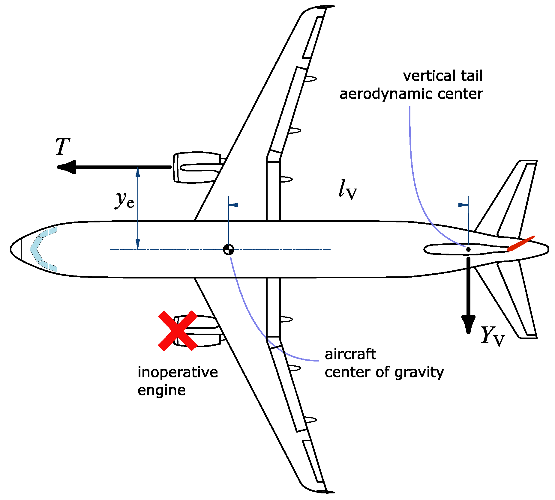
A visual representation of the forces T and Y V determining the airplane equilibrium in yaw at speed V MCa is provided by Figure 5. The critical engine, which is the most distant from the center of gravity, generates a thrust that decreases with airspeed, while the yawing moment N V = Y V · l V of the vertical tail may be expressed as:
N V = 1 2 ρ V MCa 2 S b C N δ r δ r
The most important parameters that characterize the aerodynamics of directional control are:
  • The vertical tail aspect ratio;
  • The ratio between the vertical tail span and the fuselage diameter at vertical tail aerodynamic center;
  • The horizontal tail position.
The wing has a negligible effect, because of its distance from the asymmetric flow field induced by the rudder. The rudder control power C N δ r is calculated as follows [52]:
C N δ r = C L α , V K δ r K b τ r S V S l v b η v
Here C L α , V is the isolated vertical tail lift curve slope, K δ r is the interference factor due to rudder deflection, K b is a rudder span effectiveness factor, τ r is the rudder effectiveness, η v is the vertical tail dynamic pressure ratio, and S V l V / ( S b ) is the vertical tail volumetric coefficient ( l V is the distance from the aerodynamic center of the vertical tail to the center of gravity of the airplane, as shown in Figure 5). The K b factor is a function of the rudder span-wise extension, as proposed in [53], while the rudder effectiveness τ r can be assigned as a constant or as a function of the rudder deflection according to well known classical semi-empirical approaches found in the literature [54,55]. Finally, the factor K δ r is expressed as
K δ r = 1.07 1 + K FV 1 2.2 for body mounted tail ( 1.33 0.09 A R V ) 1 + K FV 1 2.2 for T -tail configuration
where A R V is the vertical tail aspect ratio and K FV is defined as the ratio between the yawing moment coefficient of the fuselage-vertical tail combination and the yawing moment coefficient of the isolated vertical tail. The value of K FV is obtained from a surrogate model named VeDSC [52] that takes into account the interference effects due to mutual positions of the fin, fuselage, and horizontal empennage.

3.2. Landing Simulation Model

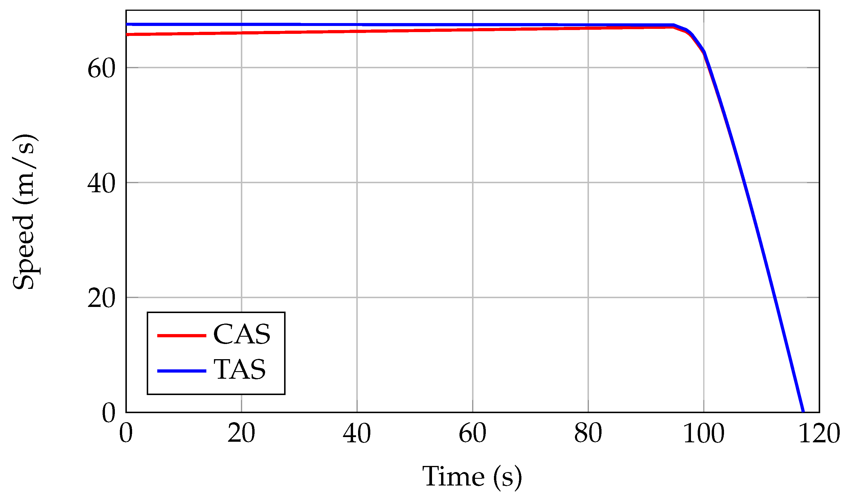
For the landing characteristics, JPAD also provides a simulation-based design approach involving the resolution of an ODE system. Landing simulations start at t = 0 s with the airplane at 1500 ft above the runway; the approach phase begins in steady flight conditions. The overall maneuver is the sequence of
  • A stabilized approach descending down to the conventional obstacle height of 50 ft;
  • A final approach down to 20 ft—that is, a smooth rotation in pitch with negligible initial variation of flight path angle;
  • A flare, with a smooth reduction of flight path angle evolving progressively into an almost horizontal trajectory;
  • A touch down and transition to ground roll;
  • A ground roll decelerating to a stop on the runway.
According to FAR regulations [56] (part 25, subpart B, paragraph 25.125), during the stabilized approach the aircraft must maintain a calibrated airspeed of not less than 1.23 times the 1-g stall speed in landing configuration; this speed must be kept all the way down to the altitude of 50 ft. Furthermore, the simulation model assumes a constant flight path angle γ for the approach, which can be assigned by the user (a typical value is 3 deg ). This angle determines the amount of thrust necessary in the simulation to keep a stabilized glide path.
At the landing obstacle altitude of 50 ft the aircraft begins the final approach down to the initial flare rotation altitude assumed to be at 20 ft above the ground, a height suggested in [57] as an averaged value for transport aircraft. In this phase, the aircraft speed must be kept almost constant and the overall thrust is changed to the flight idle setting for each engine. As a consequence, the angle of attack begins to rise during the final approach to provide for the amount of lift necessary to keep the flight path angle constant.
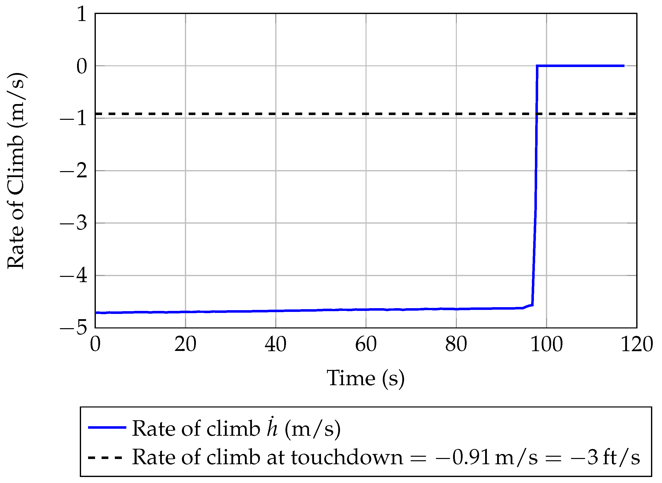
During the flare rotation a smooth transition from a normal approach attitude to a landing attitude must be accomplished by gradually rounding out the flight path to one that is parallel with the ground, and within a few inches above the runway. During this rotation the angle of attack increases, providing for higher lift and a higher induced drag resulting in a deceleration of the aircraft. At the end of the flare the airplane must touch the ground with its main landing gears and a with a reasonably low value of the vertical speed. A typical value of the descent speed at touchdown is between 2 and 3 ft/s [58]. However, as found in [58], service experience on various families of Boeing aircraft indicates that most flight crews report a hard landing when the sink rate exceeds approximately 4 ft/s. In addition, FAR regulations [59] (part 25, subpart C, paragraph 25.473) specify a limit descent velocity of 10 ft/s at the design landing weight or a limit descent velocity of 6 ft/s at the design take-off weight. To allow the user to investigate different landing scenarios, the target rate of descent at touchdown can be selected as input parameter among the ones in Table 2.
Finally, after the touchdown, and after few seconds of wheel free-roll, the pilot must apply breaking to all wheels, deflect all spoilers and adjust each engine setting to ground idle. The simulation ends when the aircraft speed reaches a value of zero.
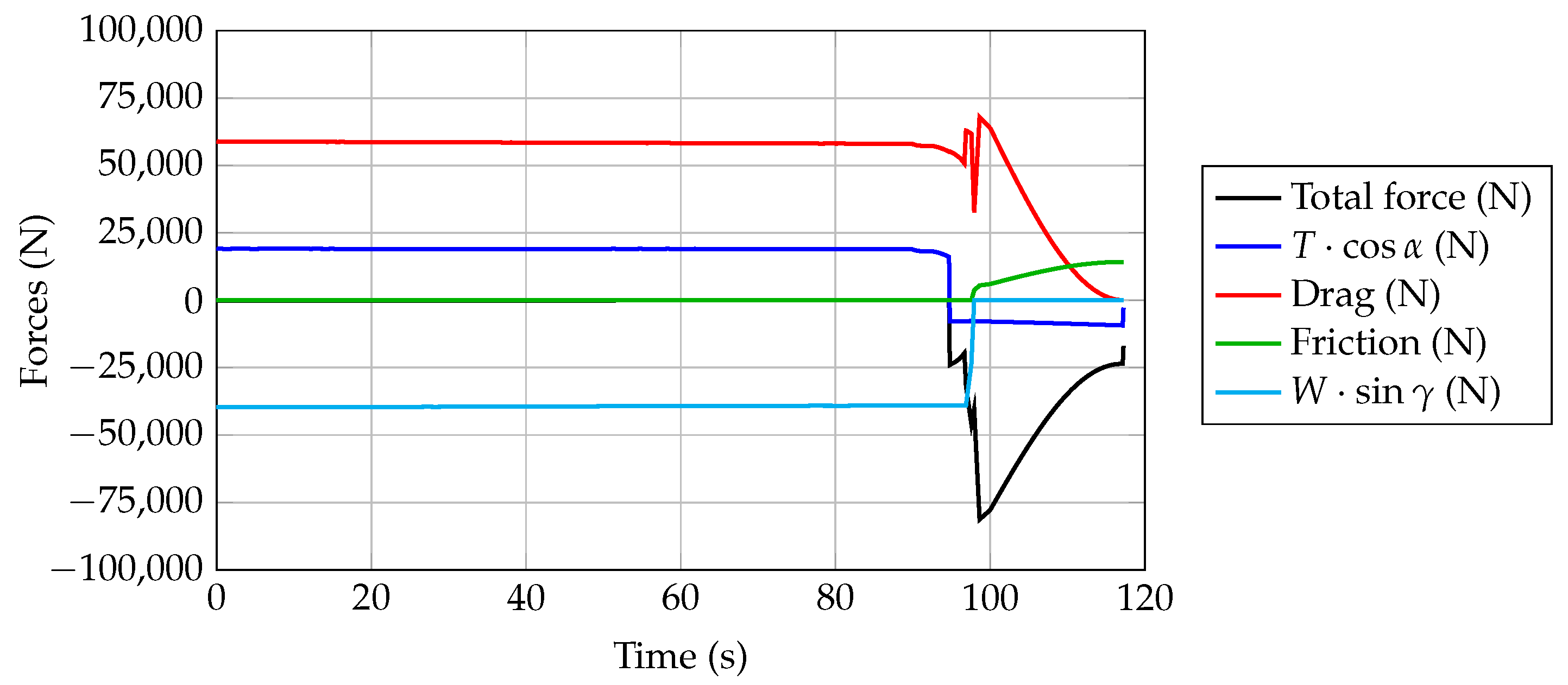
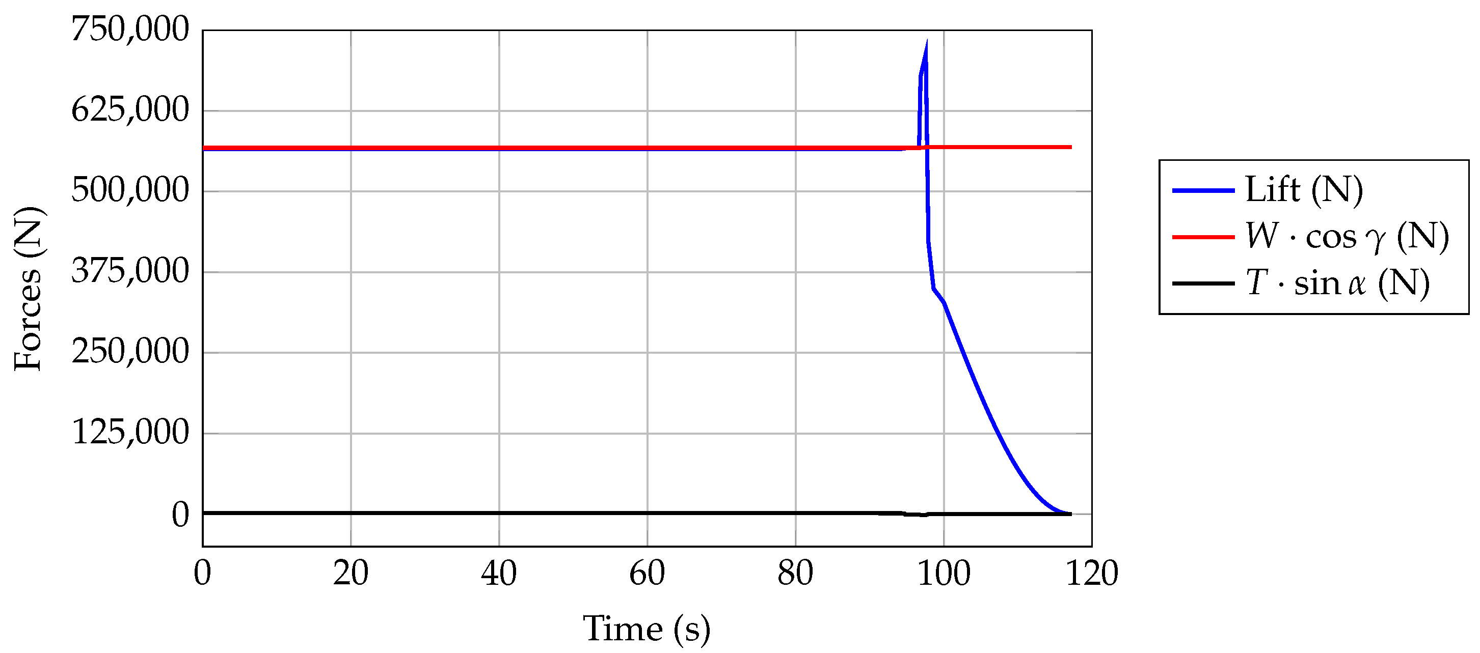
The equations of motion in case of landing are the following, where t td is the touchdown time:
f 1 V = x 2
f 2 V , γ , h , m ; α = g W T ( x 2 ) cos u W sin x 3 D ( x 2 , x 3 , x 4 , x 5 , u ) if S ( x 2 , u ) 1 ( airborne ) T ( x 2 ) D ( x 2 , x 3 , x 4 , x 5 , u ) μ W L ( x 2 , x 3 , x 4 , x 5 , u ) if S ( x 2 , u ) < 1 ( on ground )
f 3 V , γ , h , m ; α = g W x 2 L ( x 2 , x 3 , x 4 , x 5 , u ) + T ( x 2 ) sin u W cos x 3 if S ( x 2 , u ) 1 ( airborne ) 0 if S ( x 2 , u ) < 1 ( on ground )
f 4 V , γ = x 2 sin x 3
f 5 V , γ , h = m ˙ f ( x 2 , x 3 , x 4 )
The aircraft drag coefficient, calculated from the input drag polar curve in landing configuration taking into account also the ground effect, is incremented during the ground roll phase to model the effect of spoiler deflection. This additive contribution is calculated as proposed in [60], using each spoiler’s maximum deflection angle specified in the JPAD aircraft data model. Similarly, spoiler deflection also affects the lift coefficient, which is reduced by an amount dependent on each spoiler span ratio [60]. This effect provides for an increased wheel friction force, and so more effective deceleration. The increase in braking effectiveness due to spoilers may also be configured in JPAD by the user through the performance input file.
To take into account for thrust reverse during the landing simulation, the ground idle engine rating used for the ground roll phase can be modified by means of a dedicated calibration factor provided in the performance analysis input file. Otherwise, the ground idle rating of the JPAD engine database can be manually edited, including negative thrust ratios.
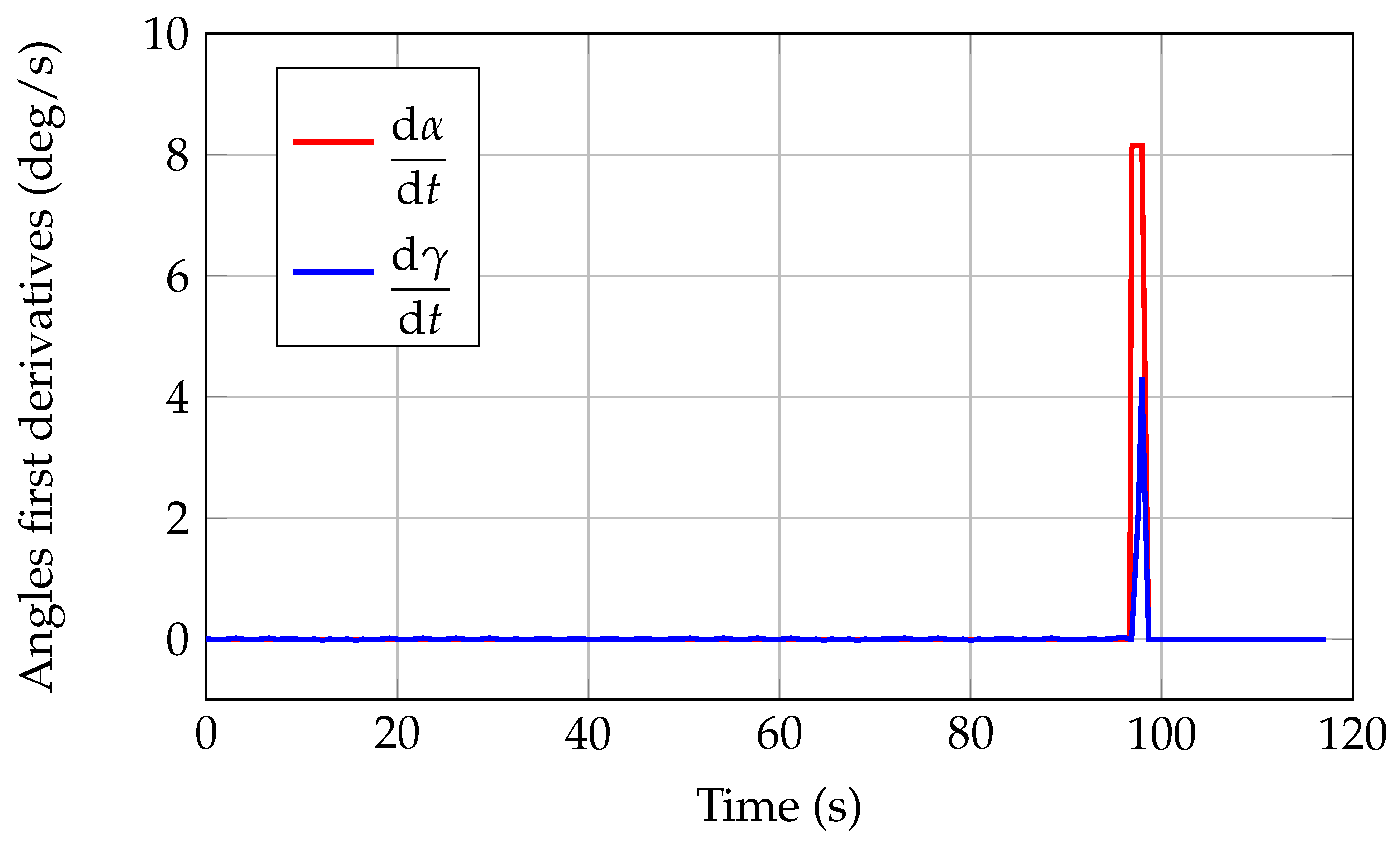
The function u ( t ) in system (9), still represents the input law of the angle of attack as a function of time and is constructed as follows:
  • At the beginning of the initial approach the angle of attack is calculated from the equilibrium lifting coefficient in landing configuration associated with the initial aircraft weight and with the prescribed approach speed of 1.23 times the stall speed at landing.
  • During both initial and final approach phases, the model implements a proportional control that senses the flight path angle γ = x 3 and regulates α to keep γ ˙ equal to zero.
  • From the height of 20 ft to touchdown a special algorithm calculates α ( t ) for the flare segment; this procedure is explained below in more detail.
  • Once the aircraft has touched the ground, a user-defined, constant value of the angle of attack is considered (this latter is set to zero degrees by default).
The flare rotation plays a very important role in the landing simulation since it must provide for a reasonable value of the vertical speed at touchdown and at the same time it has to ensure that the aircraft effectively touches the ground with a flight path angle very close to zero. The key parameter is the angle of attack time derivative, which is unknown. Thus, the following iterative process is applied to find a constant α ˙ during flare that makes the overall landing maneuver compliant with all the required conditions (see also s Figure 6 and Figure 7):
  • Two initial attempts are made assuming the impossible case of a null angle of attack time derivative and the case of α ˙ = 3 deg/s during the flare rotation. These attempts are used to make a forecast of the required pitching angular velocity to match the target value of the rate of descent. The forecast is made by using linear interpolations or extrapolations.
  • In case the simulation step should overshoot the user-defined limitation on the allowed maximum achievable lifting coefficient during landing rotation (by default set to 90% of the landing maximum lift coefficient), a warning is launched and the last calculated lift coefficient is considered.
  • In case the aircraft should touch the ground with an angle of attack bigger than the fuselage upsweep angle, a tail strike warning is launched. At the same time, if the required angle of attack time derivative should provide for an angle of attack at touchdown lower than 0 deg, a nose strike warning is launched. This feature provides for an important aircraft design check, monitoring whether the aircraft has been designed with an adequate value of the aerodynamic efficiency in landing (higher lift capabilities lead to lower angles of attack at touchdown, while poor lift capabilities provide for higher angles of attack).
  • If the aircraft reaches the required altitude and at the same time provides for a touchdown vertical speed below or equal to the threshold, the flare simulation ends, and the ground roll phase can start.
  • If flare rotation simulation fails, the JPAD performance manager switches the air distance calculation to the simpler circular arc approach proposed in [58] before then moving on to the integration of the ODE set for the final ground segment.
As for take-off simulations, JPAD provides default values of most of the simulation inputs for the landing simulation as well. However, the user has the ability to manually assign each of them. The list of inputs necessary to accomplish a landing analysis is reported in Table 3.
Starting from both take-off and landing simulations, a specific performance module has been completely dedicated to the calculation of certification take-off and landing noise trajectories. In both cases, part 36, appendix A, of the FAR [61] specifies all conditions under which aircraft noise certification tests must be conducted.

3.3. Take-Off and Landing Simulation Model for Noise Certification

The procedure for take-off noise trajectory analysis is almost the same as the AEO normal take-off, with the important difference that all simulations must be carried out considering an ISA temperature deviation of + 10   ° C . In addition to the normal take-off simulation, once the aircraft passes the obstacle at 35 ft, landing gear must be retracted. This is simulated by linearly reducing the current drag coefficient, from the trimmed drag polar in take-off configuration, of a quantity equal to the overall landing gear’s drag coefficient. The time interval assumed to perform this reduction is set by default to 12 s; however, the user can change this value in the performance analysis configuration file.
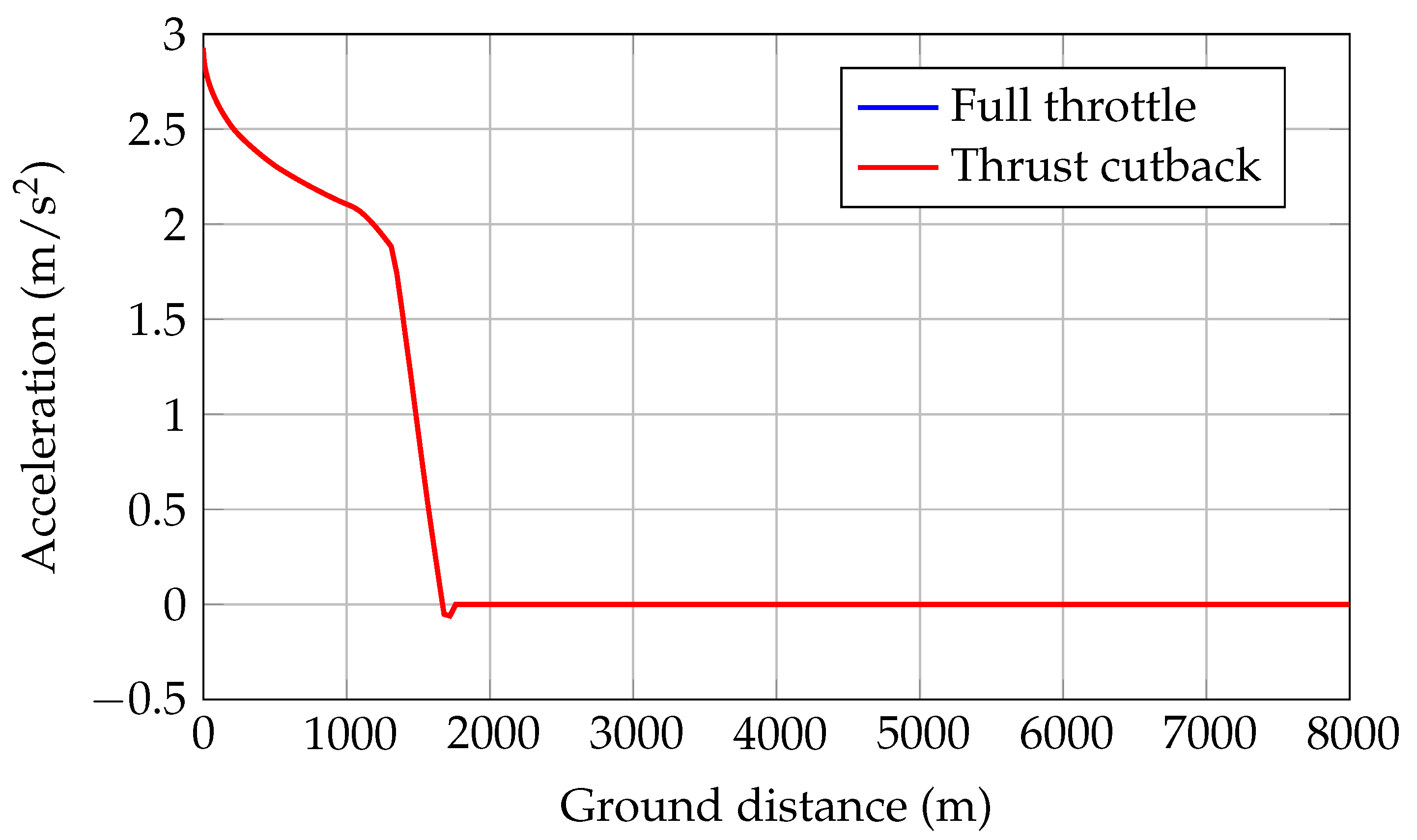
The time history of the angle of attack defined in Figure 3 is used to model the input variable u ( t ) up to the obstacle altitude. From there, the instant at which the acceleration reaches a value near to zero is monitored to estimate the aircraft speed to be maintained during the rest of the simulation. This velocity must be in the interval [ 1.13 V s , TO + 10 kts , 1.13 V s , TO + 20 kts ] . To ensure this condition in simulation, an iterative process is carried out by varying the rotation speed V rot appropriately, while making sure that in all cases the speed profile complies with all the limitations described for a normal take-off. Thus, if the calculated climb speed is less than the lower bound of the prescribed interval, the aircraft’s rotation speed is increased to allow for a higher lift-off speed. The rotation speed is reduced in the opposite case.
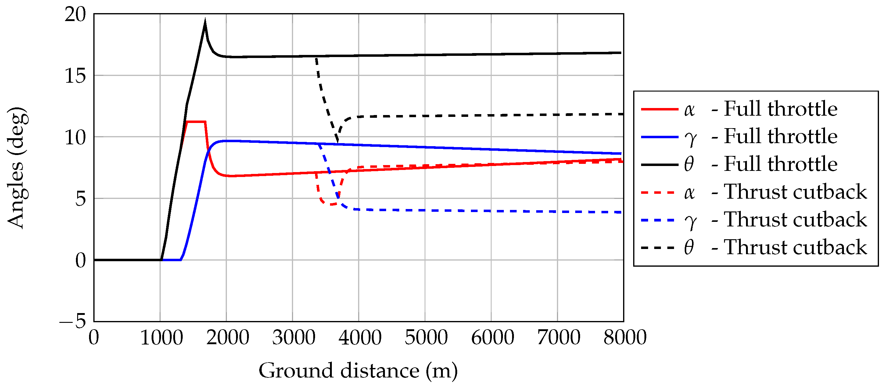
To maintain a steady climb after the obstacle, a proper law α ( t ) has to be established in order to get a constant climb speed. To ensure such behavior, the model implements a proportional control that senses the flight speed V and the rate of climb V sin γ and regulates α 
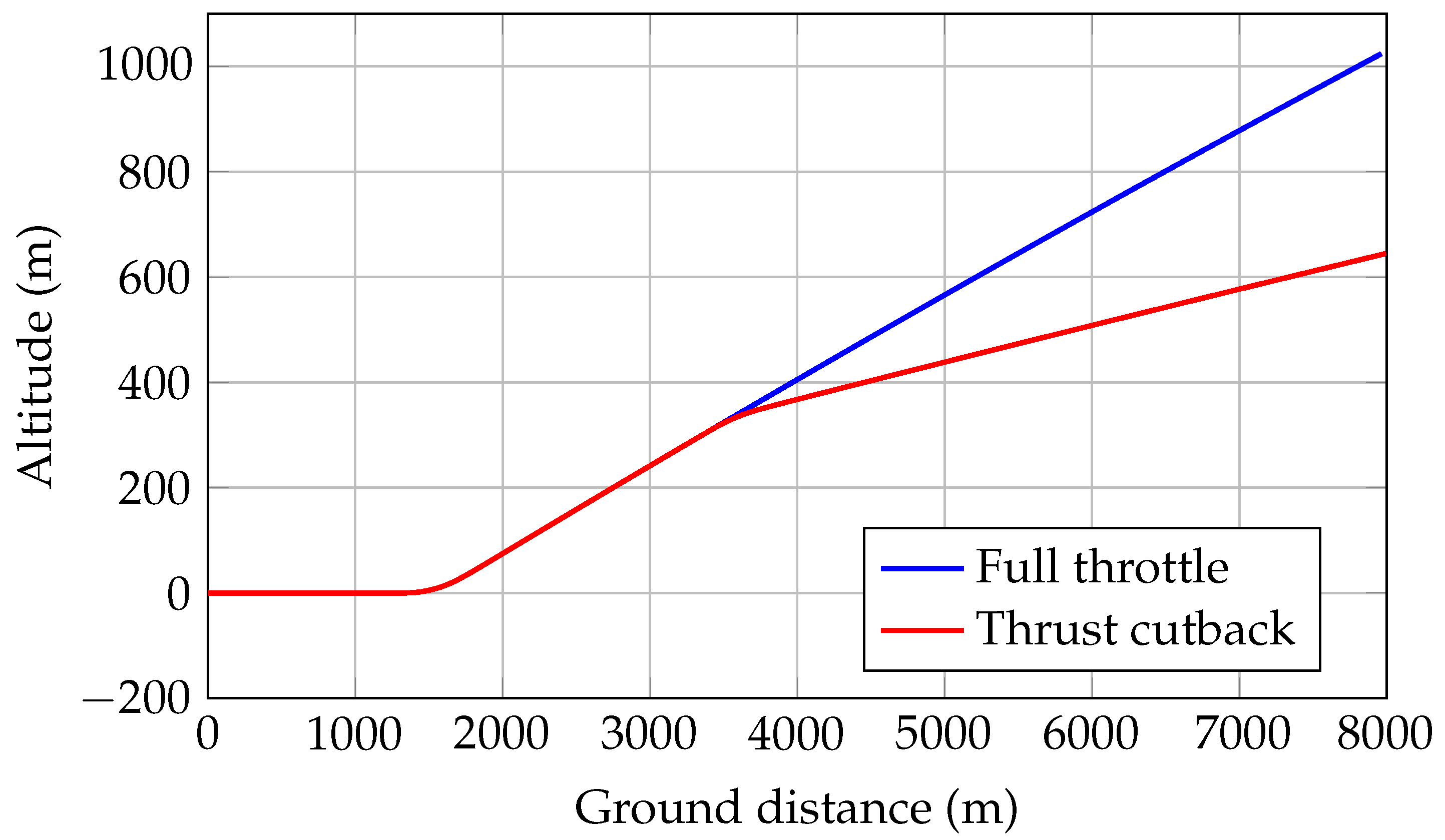
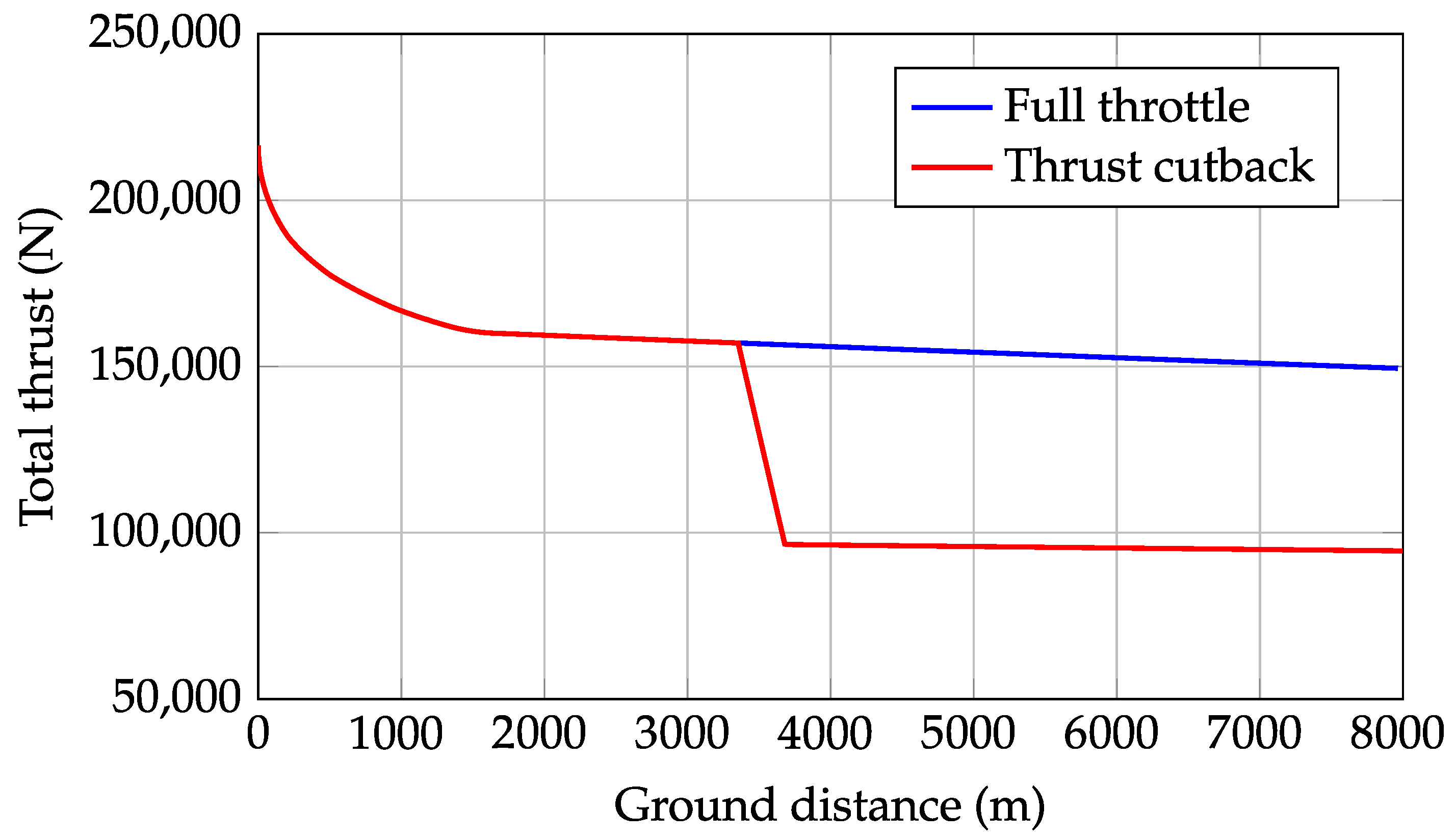
to keep their variations close to zero. Two scenarios are considered at this point: a 100% take-off thrust simulation and another one with a thrust cutback occurring at a specific altitude prescribed by regulations. The cutback altitude is selected as follows: 689 ft (210 m) for airplanes with more than three engines; 853 ft (260 m) for airplanes with three engines; and 984 ft (300 m) for airplanes with fewer than three engines. The cutback thrust setting must be selected according to the FAR [62] (Appendix B, Part 36, Section B36.7). Upon reaching the cutback altitude, the aircraft thrust is reduced, but the total amount T must not be less than the thrust required to maintain either of the following (whichever is greater): a climb gradient of 4%, and in the case of multi-engine airplanes, level flight with one engine inoperative.
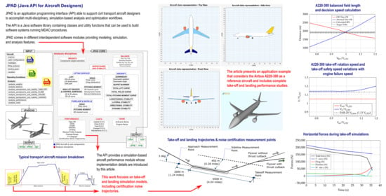
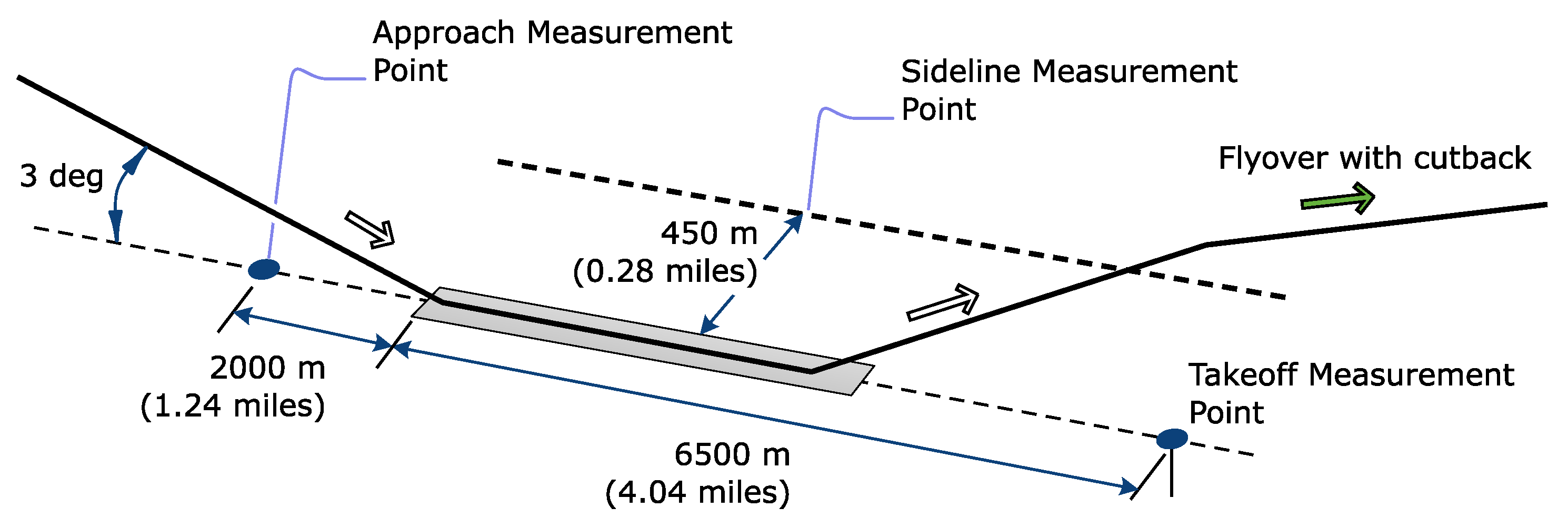
In both scenarios, 100% thrust and cutback, the simulation continues until the aircraft reaches a user-defined horizontal distance from the starting point, set by default at 8000 m. The 100% thrust case is related to the definition of a lateral noise certification point, which is that location on ground where the highest noise level is measured among all the possible measuring stations located on a line parallel to the runway center line (at a side distance of 450 m). The cutback thrust case is related to the flyover noise certification point which is set by the FAR at 6500 m from the brake-release point along the runway’s center line. Ending the simulation further than 6500 m ensures that the aircraft passes above the flyover certification point. A representation of all noise certification measurement points is provided in Figure 8, while a complete overview of the input data needed to perform both take-off noise trajectories simulation is reported in Table 4.
Landing noise trajectory simulations are practically the same as for normal landings. However, the need to only model the trajectory up to the end of the final approach allows one to completely ignore the flare and ground roll segments. According to FAR (appendix A, part 36) the approach noise certification point is defined as the location at 2300 m from the brake release (or 2000 m from the runway start) which corresponds to an aircraft altitude above the ground of 120.50 m (see Figure 8).
Both take-off and landing noise trajectories calculated using the proposed approach can be used as starting points for complete aircraft noise assessments. Thus, JPAD has been provided with an interface to an external tool named ATTILA, developed at the University of Naples Federico II, dedicated to this specific type of analysis. The noise topic lies outside the scope of this paper; however, a description of the prediction methodology implemented in this software can be found in [63], both in terms of airframe and engine noise.

4. A Take-Off and Landing Performance Simulation Example

This section presents an application of the methodologies described above and demonstrates the capabilities of JPAD concerning typical preliminary design studies. Results from the simulations of both take-off and landing phases of a regional turbofan aircraft model similar to the Airbus A220-300 will be shown. For sake of completeness, simulation details concerning the certification noise trajectories for this aircraft model will be provided as well. Those data play a very important role in the noise assessment of an aircraft model, and in fact, they represent some of the major input data that JPAD can pass to the environmental noise analysis tool ATTILA mentioned in previous section. However, thanks to the simulation-based nature of the implemented calculation methodology, output data from the JPAD certification noise trajectory analysis can be used as a starting point for any tool dedicated to the aircraft noise estimation.
The selection of the Airbus A220-300 as the reference platform was driven by two main factors: within several studies, the authors have deeply analyzed this aircraft, which represents the state-of-the-art of the current regional jet market; on the other hand, a reliable geared turbofan engine database similar to the PW1524G has been generated by the authors as a result of their involvement in recent research efforts.
The first step of this case study concerned the generation of the aircraft parametric model. Besides the main geometrical data reported in Table 5 and engine data reported in Table 6, most of the inputs needed by JPAD to define a complete aircraft model have been derived directly from the A220-330 three-view drawings through a digitization process. The cabin layout has been modeled by taking as reference the seat map presented in [64], while data concerning airfoils of lifting surfaces have been taken from [65], considering the SC(2)-0714 airfoil as wing root and kink sections and the SC(2)-0710 airfoil as tip section. In addition, a NACA 0012 has been used as root and tip airfoil for both horizontal and vertical tails.
The resulting aircraft model produced by JPAD is shown in Figure 9, where a three-view representation and a rendering of the automatically generated CAD model have been collected.
Once the aircraft model was created, the second step of this case study was related to the configuration of both take-off and landing simulations input files. It must be noted the take-off and landing presented in this paper were performed at the end of a complete JPAD multi-disciplinary analysis cycle, as shown in Figure 2. Thus, the performance module inherited all weights and trimmed aerodynamic data coming from other JPAD analysis modules. For the sake of clarity, Table 7 shows a comparison between the calculated aircraft weights and the public domain data available for the Airbus A220-300 with respect to a design mission range of 3100 nm.
Typical simulation parameters have been used for take-off and landing analyses, as well as other parameters suggested by FAR. A summary of these data is provided in Table 8.
It must be noted that the flight path angle of 4 deg reported in Table 8 was selected as the one providing for the best agreement with public data concerning the landing field length of the Airbus A220-300.
For sake of clarity, emissions data reported for both take-off and landing simulations have been obtained from dedicated lookup tables included in the JPAD engine database. Those data, as well as thrust and SFC values, have been derived by the authors in the context of past research activities and have been validated by comparison to GasTurb software [70] output data for an engine model similar to the PW1524G used for the Airbus A220-300.
In terms of take-off, Table 9 reports a summary of the JPAD simulation output, while Figure 4 illustrates the calculations of the balanced field length and of the decision speed V 1 . Furthermore, Figure 10 shows the variation of normalized rotation speed V rot / V s , TO , as well as the normalized take-off safety speed V 2 / V s , TO , with increasing engine normalized failure speed V ef / V s , TO . As can be seen, the value of the V 2 / V s , TO ratio is always above the minimum value of 1.13 prescribed by FAR.
The time histories of the main aircraft-related physical quantities during a take-off simulation are shown in Figure 11, Figure 12, Figure 13, Figure 14 and Figure 15. The assumed input rotation speed ratio of 1.05 allows one to match all rotation speed checks performed by JPAD during the take-off simulation described in the previous section of this paper. The calculated BFL of 1936 m is in line with the expected value of 1890 m available for the Airbus A220-300, with a difference of about 2.4%.
Concerning the landing analysis, input data reported in Table 8 have been used to carry out a complete simulation considering the typical case of 3 ft/s of vertical speed at touchdown. The main output data of the simulation are provided in Table 10, while Figure 16, Figure 17, Figure 18 and Figure 19 show the main physical quantities time histories. These have been reported to prove the compliance of the simulation with the specifications coming from FAR, especially the ones related to aircraft angles, speeds, and rate of descent. Moreover, the calculated landing field length of 1539 m differs from the public available A220-300 LFL value of 1509 m by less than 2%, proving the good level of accuracy reached by the proposed methodology.
Finally, some of the main results of the take-off noise trajectories simulation are provided in Figure 20, Figure 21, Figure 22 and Figure 23. Besides the two main trajectories (with and without a thrust cutback equal to 62% of the maximum take-off thrust), the provided charts show the evolutions of the aircraft’s total thrust, aircraft angles, and the overall acceleration. In particular, as seen from Figure 23, after reaching a zero acceleration for the first time, the control law implemented for the angle of attack maintained a constant speed for the rest of the simulation. This occurred in both cases of a full thrust simulation and of thrust cutback, in agreement with the classical flight test operations.
For the sake of completeness, a comparison between publicly available noise certification data for the Airbus A220-330 with results obtained by means of JPAD using the calculated noise trajectories in combination with the ATTILA tool is provided in Table 11, for the three certification points previously discussed.

5. Conclusions

Nowadays, preliminary aircraft design activities require reliable and fast calculation methods to quickly make performance assessments. Usually this task has been carried out using statistical or semi-empirical approaches which can give pretty accurate results in no time. However, those approaches may be inappropriate when dealing with innovative aircraft configurations or when a higher level of accuracy is required. Thanks to the continuous evolution of computer calculation capabilities, new and improved methodologies can now be implemented inside modern aircraft design software. An example of this can be found in the JPAD library presented in this paper.
In the framework of the development of JPAD, a detailed and flexible simulation-based analysis methodology for take-off and landing has been presented in this article. Some important simulation features not present in most of the currently available preliminary aircraft design software have received substantial attention.
An application of the proposed methodologies has been provided, considering as the reference aircraft model a state-of-the-art regional turbofan aircraft. Results, both in terms of take-off and landing simulations, are in line with public domain data related to this aircraft, proving the good level of accuracy reached by JPAD. Although far more detailed than classical semi-empirical approaches, the computational effort associated with the proposed methodologies is very limited. For the complete take-off analysis a simulation time of less than 1 s was observed; and 7.5 s was required by the landing simulation due to the touchdown vertical speed control. The benchmark was carried out on a personal computer with the following characteristics: i7-10875 octa-core CPU, 32 GB of RAM, and a 1TB Samsung EVO Plus SSD.
Thus, thanks to their increased level of accuracy and to their low computational load, the proposed methodologies can be easily used in complex multi-disciplinary analysis and optimization cycles usually required by typical preliminary aircraft design iterations.

Author Contributions

All authors contributed equally to writing this article. They teamed up to design the presented models and the associated computational framework, to analyze the data, to carry out the implementation, and finally to perform the calculation examples. All authors have read and agreed to the published version of the manuscript.

Funding

This research received no external funding.

Conflicts of Interest

The authors declare no conflict of interest.

Abbreviations

The following abbreviations are used in this manuscript:
AEOAll Engines Operative
APIApplication Programming Interface
APRAutomatic Power Reserve
ATAGAir Transport Action Group
BFLBalanced Field Length
CADComputer Aided Design
CASCalibrated Air Speed
CFDComputational Fluid Dynamics
DOCDirect Operative Cost
DOEDesign Of Experiments
EUEuropean Union
EPNLEffective Perceived Noise Level
GAGenetic Algorithm
IATAInternational Air Transport Association
ICAOInternational Civil Aviation Organization
IVPInitial Value Problem
JPADJava API for Aircraft Designers
LFLLanding Field Length
LNDLanding
LTOLanding and Take-Off
MDAOMulti-Disciplinary Design, Analysis and Optimization
MEWManufacturer’s Empty Weight
MLWMaximum Landing Weight
MTOWMaximum Take-Off Weight
MZFWMaximum Zero Fuel Weight
ODEOrdinary Differential Equation
OEIOne Engine Inoperative
OOPObject-Oriented Programming
OEWOperating Empty Weight
PSOParticle Swarm Optimization
RANSReynolds Averaged Navier–Stokes equations
RPKRevenue Passenger Kilometers
SFCSpecific Fuel Consumption
TASTrue Air Speed
TOTake-Off
TOFLTake-Off Field Length
XMLExtensible Markup Language

References

  1. Pearce, B. COVID-19 Updated Impact Assessment. Available online: https://www.iata.org/en/iata-repository/publications/economic-reports/covid-fourth-impact-assessment/ (accessed on 20 September 2020).
  2. Air Transport Bureau. Effects of Novel Coronavirus (COVID-19) on Civil Aviation: Economic Impact Analysis. Available online: https://www.icao.int/sustainability/Documents/COVID-19/ICAO_Coronavirus_Econ_Impact.pdf (accessed on 20 September 2020).
  3. Nicolosi, F.; Corcione, S.; Trifari, V.; Della Vecchia, P.; De Marco, A. Design Guidelines for High Capacity Innovative Regional Turboprop Aircraft. In Proceedings of the AIAA Scitech 2019 Forum, San Diego, CA, USA, 7–11 January 2019; American Institute of Aeronautics and Astronautics: Reston, VA, USA, 2019. [Google Scholar] [CrossRef]
  4. ATR Aircraft. Turboprop market forecast 2018–2037. 2018. Available online: http://www.atraircraft.com/turboprop-market-forecast.html (accessed on 20 September 2020).
  5. Trifari, V.; Ruocco, M.; Cusati, V.; Nicolosi, F.; De Marco, A. Multi-disciplinary analysis and optimization Java tool for aircraft design. In Proceedings of the 31st Congress of the International Council of the Aeronautical Sciences (ICAS 2018), Bangkok, Thailand, 24–26 October 2018; International Council of the Aeronautical Sciences: Bonn, Germany, 2018. [Google Scholar]
  6. TXT Group. Pacelab APD. 2019. Available online: https://www.txtgroup.com/markets/solutions/pacelab-apd/ (accessed on 20 September 2020).
  7. Stanford Aerospace Design Lab. SUAVE. 2019. Available online: http://suave.stanford.edu/ (accessed on 20 September 2020).
  8. Filippone, A. Advanced Aircraft Flight Performance; Cambridge University Press: Cambridge, UK, 2012. [Google Scholar]
  9. University of Manchester. FLIGHT. 2019. Available online: http://www.flight.mace.manchester.ac.uk/index.html (accessed on 20 September 2020).
  10. Nicolosi, F.; Paduano, G. Development of a software for aircraft preliminary design and analysis. In Proceedings of the 3rd CEAS Congress, Venice, Italy, 24–26 October 2011; Council of European Aerospace Societies: Brussels, Belgium, 2011. [Google Scholar]
  11. CFS Engineering. CEASIOM. 2019. Available online: https://www.ceasiom.com/wp/ (accessed on 20 September 2020).
  12. Zhang, M.; Rizzi, A.; Nicolosi, F.; De Marco, A. Collaborative Aircraft Design Methodology using ADAS Linked to CEASIOM. In Proceedings of the 32nd AIAA Applied Aerodynamics Conference, Atlanta, GA, USA, 16–20 June 2014; American Institute of Aeronautics and Astronautics: Reston, VA, USA, 2014. [Google Scholar] [CrossRef] [Green Version]
  13. Lissys Ltd. Piano. 2014. Available online: http://www.piano.aero/ (accessed on 20 September 2020).
  14. Optimal Aircraft Design (OAD). ADS-Aircraft Design Software. 2016. Available online: http://www.pca2000.com/en/index.php (accessed on 20 September 2020).
  15. DARCorporation. AAA-Advanced Aircraft Analysis. 2019. Available online: https://www.darcorp.com/advanced-aircraft-analysis-software/ (accessed on 20 September 2020).
  16. Raymer, D. RDS-Win Aircraft Design Software. 2019. Available online: http://www.aircraftdesign.com/rds.shtml (accessed on 20 September 2020).
  17. Martins, J.R.R.A.; Lambe, A.B. Multidisciplinary Design Optimization: A Survey of Architectures. AIAA J. 2013, 51, 2049–2075. [Google Scholar] [CrossRef] [Green Version]
  18. Kroo, I. An interactive system for aircraft design and optimization. In Proceedings of the Aerospace Design Conference, Irvine, CA, USA, 3–6 February 1992. [Google Scholar] [CrossRef]
  19. Kroo, I.; Altus, S.; Braun, R.; Gage, P.; Sobieski, I. Multidisciplinary optimization methods for aircraft preliminary design. In Proceedings of the 5th Symposium on Multidisciplinary Analysis and Optimization, Panama City Beach, FL, USA, 7–9 September 1994. [Google Scholar] [CrossRef] [Green Version]
  20. Antoine, N.E.; Kroo, I.M. Framework for Aircraft Conceptual Design and Environmental Performance Studies. AIAA J. 2005, 43, 2100–2109. [Google Scholar] [CrossRef]
  21. Allison, J.; Roth, B.; Kokkolaras, M.; Kroo, I.; Papalambros, P. Aircraft Family Design Using Decomposition-Based Methods. In Proceedings of the 11th AIAA/ISSMO Multidisciplinary Analysis and Optimization Conference, Portsmouth, VA, USA, 6–8 September 2006. [Google Scholar] [CrossRef] [Green Version]
  22. Martins, J.R.R.A.; Marriage, C. An Object-Oriented Framework for Multidisciplinary Design Optimization. In Proceedings of the 48th AIAA/ASME/ASCE/AHS/ASC Structures, Structural Dynamics, and Materials Conference, Honolulu, HI, USA, 23–26 April 2007. [Google Scholar] [CrossRef]
  23. Perez, R.E.; Jansen, P.W.; Martins, J.R. pyOpt: A Python-based object-oriented framework for nonlinear constrained optimization. Struct. Multidiscip. Optim. 2012, 45, 101–118. [Google Scholar] [CrossRef]
  24. Liem, R.P.; Kenway, G.K.W.; Martins, J.R.R.A. Multimission Aircraft Fuel-Burn Minimization via Multipoint Aerostructural Optimization. AIAA J. 2015, 53, 104–122. [Google Scholar] [CrossRef] [Green Version]
  25. Gray, J.S.; Hwang, J.T.; Martins, J.R.R.A.; Moore, K.T.; Naylor, B.A. OpenMDAO: An open-source framework for multidisciplinary design, analysis, and optimization. Struct. Multidiscip. Optim. 2015, 59, 1075–1104. [Google Scholar] [CrossRef]
  26. Gorissen, D.; Quaranta, E.; Ferraro, M.; Schumann, B.; van Schaik, J.; Gisbert, M.B.I.; Keane, A.; Scanlan, J. Value-Based Decision Environment: Vision and Application. J. Aircr. 2014, 51, 1360–1372. [Google Scholar] [CrossRef] [Green Version]
  27. Liu, H.; Tian, Y.; Zhang, C.; Yin, J.; Sun, Y. Evaluation Model of Design for Operation and Architecture of Hierarchical Virtual Simulation for Flight Vehicle Design. Chin. J. Aeronaut. 2012, 25, 216–226. [Google Scholar] [CrossRef] [Green Version]
  28. Trifari, V.; Ruocco, M.; Cusati, V.; Nicolosi, F.; De Marco, A. Java Framework for Parametric Aircraft Design—Ground Performance. Aircr. Eng. Aerosp. Technol. 2017, 89. [Google Scholar] [CrossRef] [Green Version]
  29. Nicolosi, F.; De Marco, A.; Attanasio, L.; Della Vecchia, P. Development of a Java-Based Framework for Aircraft Preliminary Design and Optimization. J. Aerosp. Inf. Syst. 2016, 13, 234–242. [Google Scholar] [CrossRef] [Green Version]
  30. Nicolosi, F.; Corcione, S.; Della Vecchia, P.; Trifari, V.; Ruocco, M. Aerodynamic design and analysis of an innovative regional turboprop configuration. In Proceedings of the 31st Congress of the International Council of the Aeronautical Sciences (ICAS 2018), Bangkok, Thailand, 24–26 October 2018; International Council of the Aeronautical Sciences: Bonn, Germany, 2018. [Google Scholar]
  31. Della Vecchia, P.; Stingo, L.; Nicolosi, F.; De Marco, A.; Daniele, E.; D’Amato, E. Application of Game Theory and Evolutionary Algorithm to the Regional Turboprop Aircraft Wing Optimization. In Proceedings of the 12th EUROGEN Conference-International Conference on Evolutionary and Deterministic Methods for Design Optimization and Control with Applications to Industrial and Societal Problems, Rhodes Island, Greece, 12–14 June 2017; ECCOMAS, European Community in Computational Methods in Applied Sciences: Paris, France, 2017. [Google Scholar]
  32. Della Vecchia, P.; Stingo, L.; Corcione, S.; Ciliberti, D.; Nicolosi, F.; De Marco, A. Game Theory and Evolutionary Algorithms Applied to MDO in the AGILE European Project. In Proceedings of the 18th AIAA/ISSMO Multidisciplinary Analysis and Optimization Conference, Denver, CO, USA, 5–9 June 2017; AIAA, American Institute of Aeronautics and Astronautics: Reston, VA, USA, 2017. [Google Scholar] [CrossRef] [Green Version]
  33. Ciliberti, D.; Della Vecchia, P.; Nicolosi, F.; De Marco, A. Aircraft Directional Stability and Vertical Tail Design: A Review of Semi-Empirical Methods. Prog. Aerosp. Sci. 2017, 95, 140–172. [Google Scholar] [CrossRef]
  34. De Marco, A.; Di Stasio, M.; Della Vecchia, P.; Trifari, V.; Nicolosi, F. Automatic modeling of aircraft external geometries for preliminary design workflows. Aerosp. Sci. Technol. 2020, 98. [Google Scholar] [CrossRef]
  35. Nicolosi, F.; Della Vecchia, P.; Trifari, V.; Di Stasio, M.; Marulo, F.; De Marco, A.; Marciello, V.; Cusati, V. Noise, Emissions and Costs trade factors for regional jet platforms using a new software for aircraft preliminary design. In Proceedings of the Aviation Technology, Integration, and Operations Conference, Lisbon, Portugal, 29–30 October 2020. [Google Scholar] [CrossRef]
  36. Coiro, D.; Nicolosi, F. Design of Low-Speed Aircraft by Numerical and Experimental Techniques Developed at DPA. Aircr. Des. J. 2001, 4, 1–18. [Google Scholar] [CrossRef]
  37. Pascale, L.; Nicolosi, F. Design and aerodynamic analysis of a light twin-engine propeller aircraft. In Proceedings of the 26th Congress of International Council of the Aeronautical Sciences, ICAS 2008, Bangkok, Thailand, 24–26 October 2018; International Council of the Aeronautical Sciences: Bonn, Germany, 2018. [Google Scholar]
  38. Nicolosi, F.; Ciliberti, D.; Della Vecchia, P.; Corcione, S. Wind tunnel testing of a generic regional turboprop aircraft modular model and development of improved design guidelines. In Proceedings of the AIAA Aviation and Aeronautics Forum and Exposition; American Institute of Aeronautics and Astronautics, Reston, VA, USA; 2018. [Google Scholar] [CrossRef] [Green Version]
  39. Della Vecchia, P.; Nicolosi, F. Aerodynamic guidelines in the design and optimization of new regional turboprop aircraft. Aerosp. Sci. Technol. (AESCTE) 2014, 38, 88–104. [Google Scholar] [CrossRef]
  40. Coiro, D.; Nicolosi, F.; Grasso, F. Design and Testing of Multi-Element Airfoil for Short-Takeoff-and-Landing Ultralight Aircraft. J. Aircr. 2009, 46, 1795–1807. [Google Scholar] [CrossRef]
  41. Della Vecchia, P.; Corcione, S.; Pecora, R.; Nicolosi, F.; Dimino, I.; Concilio, A. Design and integration sensitivity of a morphing trailing edge on a reference airfoil: The effect on high-altitude long-endurance aircraft performance. J. Intell. Mater. Syst. Struct. 2017, 28, 2933–2946. [Google Scholar] [CrossRef] [Green Version]
  42. Nicolosi, F.; Della Vecchia, P.; Ciliberti, D. Aerodynamic interference issues in aircraft directional control. J. Aerosp. Eng. 2015, 28. [Google Scholar] [CrossRef] [Green Version]
  43. Nicolosi, F.; Della Vecchia, P.; Ciliberti, D.; Cusati, V. Development of new preliminary design methodologies for regional turboprop aircraft by means of CFD analyses. In Proceedings of the 29th Congress of the International Council of the Aeronautical Sciences (ICAS 2014), Chamonix, France, 20–24 April 2014; International Council of the Aeronautical Sciences: Bonn, Germany, 2014. [Google Scholar] [CrossRef]
  44. Nicolosi, F.; Della Vecchia, P.; Corcione, S. Design and aerodynamic analysis of a twin-engine commuter aircraft. Aerosp. Sci. Technol. 2015, 40, 1–16. [Google Scholar] [CrossRef]
  45. Nicolosi, F.; Corcione, S.; Della Vecchia, P. Commuter aircraft aerodynamic characteristics through wind tunnel tests. Aircr. Eng. Aerosp. Technol. 2016, 88, 523–534. [Google Scholar] [CrossRef] [Green Version]
  46. Nicolosi, F.; De Marco, A.; Della Vecchia, P.; Sabetta, V. Roll performance assessment of a light aircraft: Flight simulations and flight tests. Aerosp. Sci. Technol. 2018, 76, 471–483. [Google Scholar] [CrossRef]
  47. Nicolosi, F.; Della Vecchia, P.; Ciliberti, D.; Cusati, V. Fuselage Aerodynamic Prediction Methods. Aerosp. Sci. Technol. (Elsevier) AESCTE 2016, 55, 322–343. [Google Scholar] [CrossRef]
  48. Schmidt, D.K. Modern Flight Dynamics; McGraw-Hill: New York, NY, USA, 2011. [Google Scholar]
  49. Hurt, H.H. Aerodynamics for Naval Aviators; FAA Handbooks Series; Federal Aviation Administration (FAA)/Aviation Supplies & Academics: Washington, DC, USA, 1992. [Google Scholar]
  50. Sforza, P. Commercial Airplane Design Principles; Elsevier: Amsterdam, The Netherlands, 2014. [Google Scholar]
  51. United States, Federal Aviation Administration. Federal Aviation Regulations. Sec. 25.107—Takeoff speeds, e, 1, ii. Available online: https://www.law.cornell.edu/cfr/text/14/25.107 (accessed on 20 September 2020).
  52. Della Vecchia, P.; Nicolosi, F.; Ciliberti, D. Aircraft directional stability prediction method by CFD. In Proceedings of the 33rd AIAA Applied Aerodynamics Conference, Dallas, TX, USA, 22–26 June 2015. [Google Scholar] [CrossRef] [Green Version]
  53. Torenbeek, E. Synthesis of Subsonic Airplane Design: An Introduction to the Preliminary Design of Subsonic General Aviation and Transport Aircraft, with Emphasis on Layout, Aerodynamic Design, Propulsion and Performance; Springer: Dordrecht, The Netherlands, 1982. [Google Scholar] [CrossRef]
  54. Fink, R. USAF Stability and Control DATCOM. Technical Report AFWAL-TR-83-3048, Wright-Patterson Air Force Base; McDonnell Douglas Corporation: Wright-Patterson AFB, OH, USA, 1978. [Google Scholar]
  55. Roskam, J. Airplane Design; DARCorporation: Lawrence, Kansas, 2000. [Google Scholar]
  56. United States, Federal Aviation Administration. Federal Aviation Regulations. Sec. 25.125—Landing, b, 2, i, A. Available online: https://www.law.cornell.edu/cfr/text/14/25.125 (accessed on 20 September 2020).
  57. Pinsker, W.J.G. The Landing Flare of Large Transport Aircraft; Technical Report Reports and Memoranda No. 3602; Aerodynamics Dept., R.A.E.: Bedford, UK, 1967; Available online: http://naca.central.cranfield.ac.uk/reports/arc/rm/3602.pdf (accessed on 20 September 2020).
  58. Young, T.M. Performance of the Jet Transport Airplane: Analysis Methods, Flight Operations, and Regulations; Aerospace Series; Wiley: Hoboken, NJ, USA, 2017. [Google Scholar]
  59. United States, Federal Aviation Administration. Federal Aviation Regulations. Sec. 25.473—Landing load conditions and assumptions, a, 2. Available online: https://www.law.cornell.edu/cfr/text/14/25.473 (accessed on 20 September 2020).
  60. Sadraey, M. Spoiler Design. Technical Report, Daniel Webster College. 2020. Available online: https://docplayer.net/25341921-Spoiler-design-mohamad-sadraey-daniel-webster-college.html (accessed on 20 September 2020).
  61. United States, Federal Aviation Administration. Federal Aviation Regulations. Appendix A to Part 36—Aircraft Noise Measurement and Evaluation Under 36.101, Appendix A, A36.2.2.2. Available online: https://www.law.cornell.edu/cfr/text/14/appendix-A_to_part_36 (accessed on 20 September 2020).
  62. United States, Federal Aviation Administration. Federal Aviation Regulations. Appendix B to Part 36—Noise Levels for Transport Category and Jet Airplanes Under 36.103, Appendix B, b36.7. Available online: https://www.law.cornell.edu/cfr/text/14/appendix-B_to_part_36 (accessed on 20 September 2020).
  63. Casale, C.; Polito, T.; Trifari, V.; Di Stasio, M.; Della Vecchia, P.; Nicolosi, F.; Marulo, F. Implementation of a Noise Prediction Software for Civil Aircraft Applications. In Proceedings of the 25th International Congress of the Italian Association of Aeronautics and Astronautics (AIDAA), Rome, Italy, 9–12 September 2019. [Google Scholar]
  64. Airport planning publication. Technical Report BD500-3AB48-32000-00 Issue 13; Airbus Canada Limited Partnership: Mirabel, QC, Canada, 2019. [Google Scholar]
  65. Schiktanz, D.; Scholz, D. Survey of Experimental Data of Selected Supercritical Airfoils. Technical Report Airport2030_TN_Supercritical_Airfoils, Aero—Aircraft Design and Systems Group Department of Automotive and Aeronautical Engineering, Hamburg University of Applied Sciences. 2011. Available online: https://www.fzt.haw-hamburg.de/pers/Scholz/Airport2030/Airport2030_TN_Supercritical_Airfoils_11-12-21.pdf (accessed on 20 September 2020).
  66. Airbus Canada Limited Partnership. A220-300 Purpose Built for Efficiency. 2019. Available online: https://www.airbus.com/aircraft/passenger-aircraft/a220-family/a220-300.html (accessed on 20 September 2020).
  67. Airbus Canada Limited Partnership. Airbus Family Figures—Farnborough 2018 Edition. 2018. Available online: https://www.airbus.com/content/dam/corporate-topics/publications/backgrounders/Airbus-Family-Figures-booklet.pdf (accessed on 20 September 2020).
  68. Type-Certificate Data Sheet for PW1500G Series Engines. Technical Report EASA.IM.E.090, European Aviation Safety Agency (EASA), Issue 7. 2019. Available online: https://www.easa.europa.eu/document-library/type-certificates/engine-cs-e/easaime090 (accessed on 20 September 2020).
  69. Pratt & Whitney. PurePower PW1500G Engine. 2018. Available online: https://newsroom.pw.utc.com/download/PW1500G.S16310.K.05.17.pdf (accessed on 20 September 2020).
  70. Kurzke, J. GasTurb. 2019. Available online: http://www.gasturb.de/index.html (accessed on 20 September 2020).
Figure 1. JPAD core architecture.
Aerospace 07 00155 g001
Figure 2. Complete JPAD analysis cycle.
Aerospace 07 00155 g002
Figure 3. Qualitative representation of the angle of attack input law.
Aerospace 07 00155 g003
Figure 4. A220-300 balanced field length and decision speed calculation—JPAD.
Aerospace 07 00155 g004
Figure 5. Qualitative representation of a two-engine aircraft with one engine inoperative and with a fully deflected rudder to ensure a constant heading.
Aerospace 07 00155 g005
Figure 6. A220-300 aircraft angles during the landing simulation—JPAD.
Aerospace 07 00155 g006
Figure 7. A220-300 aircraft angular velocities during the landing simulation—JPAD.
Aerospace 07 00155 g007
Figure 8. Certification noise measurement points.
Aerospace 07 00155 g008
Figure 9. A220-300 3-view and CAD model representation made by JPAD. (a) Top view; (b) side view;(c) front view; (d) CAD model.
Aerospace 07 00155 g009
Figure 10. A220-300 take-off rotation speed and take-off safety speed variations with engine failure speed—JPAD.
Aerospace 07 00155 g010
Figure 11. A220-300 aircraft angles during the take-off simulation—JPAD.
Aerospace 07 00155 g011
Figure 12. A220-300 aircraft angular velocities during the take-off simulation—JPAD.
Aerospace 07 00155 g012
Figure 13. A220-300 calibrated air speed (CAS) and true air speed (TAS) during the take-off simulation—JPAD.
Aerospace 07 00155 g013
Figure 14. A220-300 horizontal forces during the take-off simulation—JPAD.
Aerospace 07 00155 g014
Figure 15. A220-300 vertical forces during the take-off simulation—JPAD.
Aerospace 07 00155 g015
Figure 16. A220-300 CAS and TAS during the landing simulation—JPAD.
Aerospace 07 00155 g016
Figure 17. A220-300 rate of descent during the landing simulation—JPAD.
Aerospace 07 00155 g017
Figure 18. A220-300 aircraft horizontal forces during the landing simulation—JPAD.
Aerospace 07 00155 g018
Figure 19. A220-300 aircraft vertical forces during the landing simulation—JPAD.
Aerospace 07 00155 g019
Figure 20. A220-300 calculated take-off noise trajectories with and without thrust cutback-JPAD.
Aerospace 07 00155 g020
Figure 21. A220-300 take-off thrust evolution during the certification of noise trajectories simulation—JPAD.
Aerospace 07 00155 g021
Figure 22. A220-300 aircraft angles evolution during the certification of noise trajectories simulation—JPAD.
Aerospace 07 00155 g022
Figure 23. A220-300 aircraft acceleration during the certification of noise trajectories simulation—JPAD.
Aerospace 07 00155 g023
Table 1. Summary of take-off simulation input parameters.
Input VariablesDescription
V w Wind speed along runway (positive in case of tailwind)
μ Wheel rolling friction coefficient (constant value or function of speed)
μ b Wheel braking friction coefficient (constant value or function of speed)
Δ t hold Time interval in which the pilot must hold the bar
α g Aircraft angle of attack on the ground
h obstacle Obstacle height
k rot Percentage of the stall speed which defines the rotation speed
α ˙ 0 Initial value of the angle of attack time derivative
k C L max Safety margin with respect to the max lifting coefficient
k D , OEI Drag increment due to failed engine
k α Slope of the angle of attack time derivative in Equation (4)
Table 2. Landing simulation touchdown types.
Touchdown TypeTarget Rate of Descent
Typical3 ft/s
Perceived hard4 ft/s
Certification hard with reduced descent speed6 ft/s
Certification hard with maximum descent speed10 ft/s
Table 3. Summary of landing simulation input parameters.
Input VariablesDescription
TypeTouchdown type, defining the target rate of descent (see Table 2)
V w Wind speed along runway
μ Wheel rolling friction coefficient (constant value or function of speed)
μ b Wheel braking friction coefficient (constant value or function of speed)
k LND , weight Percentage of the max take-off weight to be used for the initial approach phase
h LND , start Initial landing altitude (by default set to 1500 ft)
h obstacle Obstacle height
γ approach Flight path angle (by default set at 3 deg )
k C L , max Safety margin with respect to the max lifting coefficient
k approach Percentage of the stall speed defining the approach speed
k flare Percentage of the stall speed defining the flare speed (circular arc approach)
k touchdown Percentage of the stall speed defining the touchdown speed (circular arc approach)
Table 4. Summary of parameters used in the simulation—take-off noise trajectories.
Input VariablesDescription
X end Ground distance at which the simulation ends.
h cutback The thrust cutback altitude.
Δ t retraction Landing gear’s retraction time interval.
Δ t cutback Time interval to pass from 100% to the cutback thrust setting.
Table 5. A220-300 main geometrical data and interior arrangements [64,66,67].
Overall length38.71 m
Overall height11.5 m
Wingspan35.1 m
Wing area112.3 m2
Fuselage diameter3.7 m
Cockpit crew2 pilots
Cabin crew3 (minimum)
Passengers130 (2-class)–160 (full economy)
Seat configuration2–3 (full economy)
Seat pitch81.3 cm (full economy)
Seat width47–48 cm (full economy)
Cargo volume31.6 m3
Cabin width3.28 m
Cabin height2.13 m
Table 6. A220-300’s main engine data [68,69].
PW1521GPW1524G
Stages1-GearBox-3-8-2-31-GearBox-3-8-2-3
BPR12:112:1
Overall length3.184 m3.184 m
Diameter, fan tip185.42 cm185.42 cm
Dry mass2177 kg2177 kg
SL Static Thrust, Take-off21,970 lbf24,400 lbf
SL Static Thrust, Max Continuous20,760 lbf23,050 lbf
SL Static Thrust, Take-off Flat RatingISA+30  C ISA+30  C
SL Static Thrust, Max Continuous Flat RatingISA+25  C ISA+25  C
Max Permissible ITT, Take-off1054  C 1054  C
Max Permissible ITT, Max Continuous1006  C 1006  C
Max Permissible Low Pressure Spool Speed10,600 rpm10,600 rpm
Max Permissible High Pressure Spool Speed24,470 rpm24,470 rpm
Min Low-Pressure Spool Speed, Flight Idle1991 rpm1991 rpm
Min Low-Pressure Spool Speed, Ground Idle1574 rpm1574 rpm
Min High-Pressure Spool Speed, Flight Idle13,264 rpm13,264 rpm
Min High-Pressure Spool Speed, Ground Idle13,264 rpm13,264 rpm
Table 7. Main output data concerning the JPAD weight analysis of the A220-300 parametric model, compared with publicly available data.
Output DataJPADA220-330Difference (%)
MTOW68,272 kg67,585 kg 1.01 %
MLW58,036 kg58,740 kg 1.19 %
Max fuel mass17,739 kg17,726 kg 1.00 %
Design mission fuel mass16,833 kg
MZFW55,694 kg55,792 kg 0.17 %
Max payload18,711 kg18,711 kg0%
Design payload14,462 kg
OEW36,983 kg37,081 kg 0.39 %
Trapped fuel and oil mass341 kg
Crew mass517 kg
Operating items mass2096 kg
MEW30,705 kg
Structural mass19,841 kg
Table 8. Input parameters used for take-off and landing simulations.
Take-off
V w 0 m/s
μ 0.025
μ b 0.4
Δ t hold 0.5 s
α g 0 deg
h obstacle 35 ft
k rot 1.05
α ˙ 0 3 deg/s
k C L , max 0.8
k Drag , OEI 0.0050
k α 0.04
Landing
TypeTypical
V w 0 m/s
μ 0.025
μ b 0.4
k LND , weight 0.85
h LND , start 1500 ft
h obstacle 50 ft
γ approach 4 deg
k C L , max 0.9
k approach 1.23
k flare 1.19
k touchdown 1.15
Table 9. Main output data concerning the JPAD take-off simulation of the A220-300.
OutputValue
Ground roll distance1034 m
Rotation distance358 m
Airborne distance194 m
AEO take-off distance1586 m
FAR-25 take-off distance (take-off distance times 1.15)1824 m
BFL1936 m
V MC 54.69 m/s
V s , TO 67.01 m/s
V 1 66.61 m/s
V rot 70.36 m/s
V LO 79.26 m/s
V 2 82.71 m/s
V MC / V s , TO 0.82
V 1 / V s , TO 0.99
V rot / V s , TO 1.05
V LO / V s , TO 1.18
V 2 / V s , TO 1.23
Take-off duration35 s
Fuel used for take-off54.29 kg
Take-off NOx emissions1.27 kg
Take-off CO2 emissions184.39 kg
Take-off H2O emissions67.87 kg
Table 10. Main output data concerning the JPAD landing analysis of the A220-300.
OutputValue
Airborne distance133 m
Flare rotation distance84 m
Ground roll distance706 m
Landing distance923 m
FAR-25 LFL1539 m
Total landing distance (from 1500 ft)7313 m
V s , LND 54.92 m/s
V approach 67.45 m/s
V flare 66.72 m/s
V td 65.79 m/s
V approach / V s , LND 1.23
V flare / V s , LND 1.21
V td / V s , LND 1.20
Vertical speed at touchdown 0.91 m/s ( 3 ft/s)
Total landing duration (from 1500 ft)117 s
Landing duration23 s
Total Fuel used (from 1500 ft)40.61 kg
Total NOx emissions1.59 kg
Total CO2 emissions128.39 kg
Total H2O emissions50.76 kg
Table 11. Comparison between publicly available equivalent perceived noise level data certified for A220-330 and JPAD output using the ATTILA tool [63].
JPAD-ATTILAA220-330 Certification Data
Approach EPNL 93.1 dB 92.4 dB
Flyover EPNL 81.1 dB 80.5 dB
Lateral EPNL 88.1 dB 87.3 dB
Publisher’s Note: MDPI stays neutral with regard to jurisdictional claims in published maps and institutional affiliations.

