Article

Dot Product Equality Constrained Attitude Determination from Two Vector Observations: Theory and Astronautical Applications

1
Department of Electronic and Computer Engineering, Hong Kong University of Science and Technology, Hong Kong, China
2
Department of Aerospace Science and Technology, Space Engineering University, Beijing 101416, China
*
Author to whom correspondence should be addressed.
Aerospace 2019, 6(9), 102; https://doi.org/10.3390/aerospace6090102
Submission received: 4 July 2019 / Revised: 6 September 2019 / Accepted: 9 September 2019 / Published: 12 September 2019
(This article belongs to the Special Issue Spacecraft Attitude Determination and Control)

Abstract

:
In this paper, the attitude determination problem from two vector observations is revisited, incorporating the redundant equality constraint obtained by the dot product of vector observations. Analytical solutions to this constrained attitude determination problem are derived. It is found out that the studied two-vector attitude determination problem by Davenport q-method under the dot product constraint has deterministic maximum eigenvalue, which leads to its advantage in error/perturbation analysis and covariance determination. The proposed dot product constrained two-vector attitude solution is applied then to solve several engineering problems. Detailed simulations on spacecrafts attitude determination indicate the efficiency of the proposed theory.

1. Introduction

Attitude determination from vector observations is usually employed in astronautical applications for state estimation and control of spacecrafts [1,2,3]. Commonly, the vector observations are acquired from vector-measurement sensors e.g., Sun sensor, Nadir sensor, magnetometer, star tracker, etc. [4,5,6]. The usage of direct attitude determination from such sensors has the advantage of compensating for biases in rate gyroscopes to cancel the long-endurance drifts inside inertial navigation results [7,8].
In the past several decades, many algorithms for optimal attitude determination have been developed [9,10]. Apart from some intuitive geometric approaches, most of the others are based on the Wahba’s problem posed in 1965, giving optimal attitude matrix estimates with normalized vector measurements along with their statistical weights [11]. There have been a lot of Wahba’s solvers developed in the past 30 years, including celebrated ones such as the QUaternion ESTimator (QUEST [12]), singular value decomposition (SVD [13]) and Euler-q [14], and recent ones such as the vector-inertia-based method by Patera [15], the Riemannian-manifold-based on by Yang [16], the optimal linear estimator of quaternion (OLEQ [17]), etc. These solver are all general ones facing the multivector cases. Actually, when there are few pairs of vector observations, the Wahba’s optimization can also be solved via numerical algorithms like gradient-descent algorithm (GDA [18]), Gauss–Newton algorithm (GNA [19]), Levenberg–Marquardt algorithm (LMA [20]), etc. Such optimization-based solvers are popular in mechatronic navigation tasks with accelerometers and magnetometers only [21].
It was found that with two vector observation pairs, we can compute the full attitude results using the methods such as TRIAD [22]. For instance, with a sun sensor and a magnetometer, the full attitude angles along with the orbit can already be determined accurately [23,24]. Based on the two-vector case, Markley has developed two approaches [25,26]. For the very first one, the attitude quaternion is employed for parameterizing the orientation transformation; and, in the second one, the optimal attitude matrix of such problem has been successfully found out. Markley’s methods are proven to be efficient in engineering practice. These two optimized approaches are all based on conventional Wahba’s framework and can not improve the essential accuracy. However, for some two-vector based attitude determination system, e.g., accelerometer–magnetometer-based one, the magnetometer’s reference vector for true-north-finding is determined by the absolute position of the object in Earth coordination system [27]. Commonly, when there is no magnetic distortion, the attitude results will be quite reliable. When adding some magnetic interferences, all Euler angles using a true-north reference vector will all be disturbed, thus generating large attitude biases. However, the accelerometer can independently determine the roll and pitch angles, which indicates that the disturbances from magnetic sensing can be separated. In the work by the authors of [28], this is achieved by introducing an equality constraint formed by vector dot product from rigid-body motion; whereas, the two-vector attitude determination system is far beyond the single accelerometer–magnetometer one, it is believed that there might be some more generalized theory inside such two-vector system with dot product equality constraint, as some system dynamics will be interesting by incorporating external equality constraints, e.g., the works by the authors of [29,30,31].
Guided by the aforementioned problem, in this paper, we present a novel attitude determination algorithm from two vector observations. The framework is still within the Wahba’s optimization, but is penalized by adding a dot product equality constraint derived from vector relations. We also show that under the proposed conditions of dot product constraint, the loss function of Wahba’s problem can be reduced to 0, i.e., the sensors can extract self information to for possible maximum separation of different sensor effects and angle observabilities. The proposed two-vector approach can be an alternative for spacecraft attitude determination backup that subjects to the minimum equipment list (MEL).
The remainder of the paper is organized as follows. Section 2 contains problem backgrounds. Section 3 includes our main results on the studied problem. Section 4 consists an astronautical application and some related experimental results. In Section 5, we draw the concluding remarks.

2. Problem Fomulation

Given two normalized vector observation pairs in the body frame b and reference frame r, one can relate them by
b 1 = C r 1 b 2 = C r 2
where C in the special orthogonal group S O ( 3 ) : = { C | C T C = I , det ( C ) = 1 } is the direction cosine matrix (DCM); the sensor measurements are given by
b 1 = b x , 1 , b y , 1 , b z , 1 T r 1 = r x , 1 , r y , 1 , r z , 1 T , b 2 = b x , 2 , b y , 2 , b z , 2 T r 2 = r x , 2 , r y , 2 , r z , 2 T
provided that
b x , 1 2 + b y , 1 2 + b z , 1 2 = 1 r x , 1 2 + r y , 1 2 + r z , 1 2 = 1 b x , 2 2 + b y , 2 2 + b z , 2 2 = 1 r x , 2 2 + r y , 2 2 + r z , 2 2 = 1
In astronautical missions, the spacecraft is always equipped with a Sun sensor, magnetometer, horizon sensor, etc. for attitude determination (see Figure 1). Wahba’s problem aims to find out the optimal DCM of Equation (1) by the following least-square optimization.
arg min C S O ( 3 ) w b 1 C r 1 2 + ( 1 w ) b 2 C r 2 2
where w is the weight belonging to the first vector observation pair. This optimization can be reduced to finding the optimal eigenvector of the following matrix K [32,33],
K = B + B T t r ( B ) I z z T t r ( B )
such that
Kq = λ max q
where λ max is the largest eigenvalue of K while other parameters are given by
B = w b 1 r 1 T + ( 1 w ) b 2 r 2 T z = w b 1 × r 1 + ( 1 w ) b 2 × r 2
The characteristic polynomial of K can be computed by
det ( K λ I ) = 0
In fact, many closed-form formulations of this polynomial have been developed. For instance, in ESOQ2, it has been given that [34,35]
λ 4 + τ 1 λ 2 + τ 2 λ + τ 3 = 0
where
τ 1 = 2 t r 2 ( B ) + t r a d j ( B + B T ) z T z τ 2 = t r a d j ( K ) τ 3 = det ( K )
where a d j denotes the adjoint matrix. In the following sections, we derive the analytical solution to λ max while generating some internal perspectives on the relationship between body and reference vectors.

3. Proposed Theory

3.1. Dot Product-Equality Constraint

Theorem 1.
Defining
H x 1 H x 2 H x 3 H y 1 H y 2 H y 3 H z 1 H z 2 H z 3 = B T
the following matrix [36],
W 1 , 1 = H x 1 + H y 2 + H z 3 W 1 , 2 = H y 3 + H z 2 W 1 , 3 = H z 1 + H x 3 W 1 , 4 = H x 2 + H y 1 W 2 , 1 = H y 3 + H z 2 W 2 , 2 = H x 1 H y 2 H z 3 W 2 , 3 = H x 2 + H y 1 W 2 , 4 = H x 3 + H z 1 W 3 , 1 = H z 1 + H x 3 W 3 , 2 = H x 2 + H y 1 W 3 , 3 = H y 2 H x 1 H z 3 W 3 , 4 = H y 3 + H z 2 W 4 , 1 = H x 2 + H y 1 W 4 , 2 = H x 3 + H z 1 W 4 , 3 = H y 3 + H z 2 W 4 , 4 = H z 3 H y 2 H x 1
where W i , j denotes the matrix entry of W with row and column indices of i and j respectively, has the similar structure with K and owns the same eigenvalues and associated eigenvectors.
Proof. 
We can directly obtain
B + B T t r ( B ) I = H x 1 H y 2 H z 3 H x 2 + H y 1 H x 3 + H z 1 H x 2 + H y 1 H y 2 H x 1 H z 3 H y 3 + H z 2 H x 3 + H z 1 H y 3 + H z 2 H z 3 H y 2 H x 1 t r ( B ) = H x 1 + H y 2 + H z 3 z = B 2 , 3 B 3 , 2 , B 3 , 1 B 1 , 3 , B 1 , 2 B 2 , 1 T = H y 3 + H z 2 , H z 1 + H x 3 , H x 2 + H y 1 T
Comparing the above results with Equation (12), we have
W = t r ( B ) z T z B + B T t r ( B ) I
It is evident that W and K has the similar structure. This completes the proof. □
Lemma 1.
τ 2 = 0 holds for arbitrary two pairs of vector observations.
Proof. 
The diagonal elements of K matrix can be given by
K 1 , 1 = b z , 2 r z , 2 + b y , 2 r y , 2 b x , 2 r x , 2 ( w 1 ) + b x , 1 r x , 1 b y , 1 r y , 1 b z , 1 r z , 1 w K 2 , 2 = b z , 2 r z , 2 b y , 2 r y , 2 + b x , 2 r x , 2 ( w 1 ) + b x , 1 r x , 1 + b y , 1 r y , 1 b z , 1 r z , 1 w K 3 , 3 = b z , 2 r z , 2 + b y , 2 r y , 2 + b x , 2 r x , 2 ( w 1 ) + b x , 1 r x , 1 b y , 1 r y , 1 + b z , 1 r z , 1 w K 4 , 4 = b z , 2 r z , 2 b y , 2 r y , 2 b x , 2 r x , 2 ( w 1 ) + b x , 1 r x , 1 + b y , 1 r y , 1 + b z , 1 r z , 1 w
Therefore, it is obvious that the sum of the eigenvalues to K equals to K 1 , 1 + K 2 , 2 + K 3 , 3 + K 4 , 4 = 0 . This is why the coefficient of λ 3 is zero. Note that τ 2 is de facto in the form of [36]
τ 2 = 8 H x 3 H y 2 H z 1 H x 2 H y 3 H z 1 H x 3 H y 1 H z 2 + H x 1 H y 3 H z 2 + H x 2 H y 1 H z 3 H x 1 H y 2 H z 3
Actually, the right part can be represented by
τ 2 = 8 det ( B )
In view of B for the two-vector case, we can see that it takes the following form
B = w b 1 r 1 T + ( 1 w ) b 2 r 2 T r a n k ( B ) r a n k w b 1 r 1 T + r a n k ( 1 w ) b 2 r 2 T = 2
indicating that B is rank-deficient. Therefore, we arrive at
τ 2 = 8 det ( B ) = 0
which completes the proof. □
With Lemma 1, we can see that the characteristic polynomial is essentially a quadratic equation of λ 2 . Then the eigenvalues can be solved immediately via
λ = ± τ 1 ± τ 1 2 4 τ 3 2
The maximum eigenvalue should be
λ max = τ 1 + τ 1 2 4 τ 3 2
because [36]
τ 1 = 2 H x 1 2 + H x 2 2 + H x 3 2 + H y 1 2 + H y 2 2 + H y 3 2 + H z 1 2 + H z 2 2 + H z 3 2 < 0
As the q-method is derived from the Lagrange multiplier, with increasing maximum eigenvalue, the loss function becomes even smaller. The maximum eigenvalue has an upper bound, as proven by Shuster that [12]
λ max i = 1 n w i = 1
where w i is the weight of the i-th vector observation pair. Regarding λ max as a function of the vector observations, we can seek its largest point. This is equivalent to figuring out the solution to the following system,
2 λ max 2 b x , 1 = 0 2 λ max 2 b y , 1 = 0 2 λ max 2 b z , 1 = 0 , 2 λ max 2 b x , 2 = 0 2 λ max 2 b y , 2 = 0 2 λ max 2 b z , 2 = 0 , 2 λ max 2 r x , 1 = 0 2 λ max 2 r y , 1 = 0 2 λ max 2 r z , 1 = 0 , 2 λ max 2 r x , 2 = 0 2 λ max 2 r y , 2 = 0 2 λ max 2 r z , 2 = 0
which is rather difficult in detail. Let us write out the algebraic form of τ 1 and τ 3 :
τ 1 = 2 + 4 w 4 w 2 + 4 w ( w 1 ) b x , 1 b x , 2 + b y , 1 b y , 2 + b z , 1 b z , 2 r x , 1 r x , 2 + r y , 1 r y , 2 + r z , 1 r z , 2
τ 3 = 1 4 w + 12 w 2 16 w 3 + 8 w 4 4 w ( w 1 ) b x , 1 b x , 2 + b y , 1 b y , 2 + b z , 1 b z , 2 r x , 1 r x , 2 + r y , 1 r y , 2 + r z , 1 r z , 2 + 8 w 2 ( w 1 ) b x , 1 b x , 2 + b y , 1 b y , 2 + b z , 1 b z , 2 r x , 1 r x , 2 + r y , 1 r y , 2 + r z , 1 r z , 2 8 w 3 ( w 1 ) b x , 1 b x , 2 + b y , 1 b y , 2 + b z , 1 b z , 2 r x , 1 r x , 2 + r y , 1 r y , 2 + r z , 1 r z , 2 4 w 2 ( w 1 ) 2 b y , 1 2 2 b x , 1 b x , 2 b y , 1 b y , 2 + b y , 2 2 2 b y , 1 2 b y , 2 2 + b z , 1 2 b y , 2 2 b z , 1 2 2 b x , 1 b x , 2 b z , 1 b z , 2 2 b y , 1 b y , 2 b z , 1 b z , 2 + b z , 2 2 b y , 1 2 b z , 2 2 2 b z , 1 2 b z , 2 2 + r y , 1 2 2 r x , 1 r x , 2 r y , 1 r y , 2 + r y , 2 2 2 r y , 1 2 r y , 2 2 + r z , 1 2 r y , 2 2 r z , 1 2 2 r x , 1 r x , 2 r z , 1 r z , 2 2 r y , 1 r y , 2 r z , 1 r z , 2 + r z , 2 2 r y , 1 2 r z , 2 2 2 r z , 1 2 r z , 2 2
Note that we have the following simplification.
b y , 1 2 + b z , 1 2 + b y , 2 2 + b z , 2 2 b y , 1 2 b y , 2 2 b y , 2 2 b z , 1 2 b y , 1 2 b z , 2 2 b z , 1 2 b z , 2 2 = b y , 1 2 + b z , 1 2 + b y , 2 2 + b z , 2 2 b y , 1 2 + b z , 1 2 b y , 2 2 + b z , 2 2 = 2 b x , 1 2 b x , 2 2 1 b x , 1 2 1 b x , 2 2 = 2 b x , 1 2 b x , 2 2 1 b x , 1 2 b x , 2 2 + b x , 1 2 + b x , 2 2 = 1 b x , 1 2 b x , 2 2
With
p = b 1 · b 2 = b x , 1 b x , 2 + b y , 1 b y , 2 + b z , 1 b z , 2 q = r 1 · r 2 = r x , 1 r x , 2 + r y , 1 r y , 2 + r z , 1 r z , 2
τ 1 and τ 3 are simplified to
τ 1 = 2 + 4 w 4 w 2 + 4 w ( w 1 ) p q τ 3 = 1 4 w + 12 w 2 16 w 3 + 8 w 4 4 w 1 2 w + 2 w 2 ( w 1 ) p q 4 w 2 ( w 1 ) 2 2 p 2 q 2
Therefore, it is shown that the eigenvalue is actually the function of p and q, with parameters ranging from
p = b 1 · b 2 1 , 1 q = r 1 · r 2 1 , 1 w 0 , 1
The figures of the maximum eigenvalue Equation (21) with w = 0.5 are depicted as follows in Figure 2.
With different w, the maximum eigenvalues are drawn in Figure 3.
From the above figures, we see that the maximum eigenvalue is a convex function with respect to p and q no matter how w changes. Based on this point, the global optimum-seeking procedure is then reduced to solve the following system.
2 λ max 2 p = 0 2 λ max 2 q = 0
The partial differentiation can be computed by
2 λ max 2 r = τ 1 r + 1 2 τ 1 2 4 τ 3 2 τ 1 τ 1 r 4 τ 3 r
where r is the differentiation independent variables:
r = p , q
By which the specific derivatives are obtained by
τ 1 p = 4 w ( w 1 ) q τ 1 q = 4 w ( w 1 ) p , τ 3 p = 4 w 1 2 w + 2 w 2 ( w 1 ) q + 8 w 2 ( w 1 ) 2 p τ 3 q = 4 w 1 2 w + 2 w 2 ( w 1 ) p + 8 w 2 ( w 1 ) 2 q
Inserting these equalities into Equation (30) and invoking
2 λ max 2 r = 0 τ 1 r = 1 τ 1 2 4 τ 3 τ 1 τ 1 r 2 τ 3 r τ 1 2 4 τ 3 2 τ 1 2 τ 1 r = τ 3 r
we obtain
p = q
at which, we also have
τ 1 2 4 τ 3 = 4 w 4 w 2 + 4 w ( w 1 ) p q
leading to
λ max = 1
Reconsidering the forms of p and q, we find out
p = q b 1 · b 2 = r 1 · r 2
which can actually be derived from another aspect by
b 1 · b 2 = b 1 T b 2 = r 1 T C T C r 2 = r 1 T r 2 = r 1 · r 2
This finding reflects that the equality constraint Equation (38) can achieve least value of Wahba’s loss function, such that [32]
L ( C ) = w b 1 C r 1 2 + ( 1 w ) b 2 C r 2 2 = 1 t r ( C B T ) = 1 q T Kq = 1 q T λ max q = 0
The occurrence of λ max = 1 has in fact been shown by Markley [26]. However, we need to note that the attitude matrix employed for attitude representation in the work by the authors of [26] is not as flexible as the quaternion used in this paper, as a quaternion only requires normalization rather than orthonormalization for an attitude matrix [37].

3.2. Quaternion Solution

As the loss function is zero, we can regard the optimization as a properly solved one. That is, at this time, the information from each sensor has been maximumly extracted to reduce the loss function value; and, geometrically, every sensor has fully contributed to all those angles that they can observe. This means the optimal quaternion is finally computed via
K I q = 0
generating the following row-echelon form
K I 1 α / N 1 β / N 1 γ / N 0
The symbolic solutions to this function can be obtained by
N = 1 b y , 1 r y , 1 b y , 2 r y , 2 + b z , 1 r z , 1 + b z , 2 r z , 2 + b x , 1 r y , 1 b x , 1 r x , 1 r y , 2 2 + q 2 r x , 2 r y , 1 b y , 2 r x , 1 b x , 2 r y , 1 + b x , 2 b y , 1 b x , 1 b y , 2 + r y , 2 r y , 1 b x , 1 r y , 2 + b x , 1 r x , 2 + b y , 2 r y , 1 + b y , 1 r y , 2 + r x , 1 r y , 2 b y , 1 r x , 2 + b x , 2 r y , 1 b x , 2 b y , 1 + b x , 1 b y , 2 + r x , 2 r z , 1 b z , 2 r x , 1 b x , 2 r z , 1 b x , 2 b z , 1 + b x , 1 b z , 2 + r x , 1 r z , 2 b z , 1 r x , 2 b x , 1 r z , 2 + b x , 2 b z , 1 b x , 1 b z , 2 + r z , 1 r z , 2 b x , 2 r x , 1 + b x , 1 r x , 2 b z , 2 r z , 1 b z , 1 r z , 2 + r y , 1 r z , 2 b z , 1 r y , 2 + b y , 2 r z , 1 + b y , 2 b z , 1 b y , 1 b z , 2 + r y , 2 r z , 1 b z , 2 r y , 1 + b y , 1 r z , 2 b y , 2 b z , 1 + b y , 1 b z , 2
α = b z , 2 r x , 1 r x , 2 r y , 1 + b x , 2 b y , 1 r x , 2 r z , 1 b y , 2 r x , 1 r x , 2 r z , 1 b x , 2 b y , 1 r x , 1 r z , 2 b y , 1 r x , 1 r x , 2 r z , 2 + b x , 1 b z , 2 r x , 2 r y , 1 b z , 2 r x , 1 r y , 2 b y , 2 r x , 2 r z , 1 + b y , 2 r x , 1 r z , 2 + b z , 1 r y , 2 b x , 2 r x , 1 + r x , 2 r x , 1 + r z , 1 r z , 2 + r y , 1 b x , 2 r x , 2 + r y , 2 2 1 + b z , 2 r y , 2 r y , 1 2 b y , 2 r y , 2 r y , 1 r z , 1 b y , 1 r y , 2 r y , 1 r z , 2 + b z , 2 r y , 1 r z , 1 r z , 2 b y , 1 r z , 1 r z , 2 2 b z , 2 r y , 2 + b y , 1 r z , 1 b y , 2 r z , 1 2 r z , 2 + b y , 2 r z , 2
β = b z , 2 r x , 2 r y , 1 2 b z , 2 r x , 1 r y , 2 r y , 1 b z , 1 r x , 2 r y , 2 r y , 1 + b x , 2 r y , 2 r y , 1 r z , 1 + b x , 1 r y , 2 r y , 1 r z , 2 + b z , 1 r x , 1 r y , 2 2 + b y , 2 b z , 1 r x , 2 r y , 1 + b x , 1 r y , 1 r z , 2 + b z , 1 r x , 1 r y , 2 b x , 1 r y , 2 r z , 1 + b y , 1 b z , 2 r x , 2 r y , 1 b x , 2 r y , 1 r z , 2 b z , 2 r x , 1 r y , 2 + b x , 2 r y , 2 r z , 1 + b z , 2 r x , 2 r z , 1 2 + b z , 1 r x , 1 r z , 2 2 + b x , 1 r z , 1 r z , 2 2 b x , 1 r z , 1 + b x , 2 r x , 1 r x , 2 r z , 1 + b x , 2 r z , 1 2 r z , 2 b x , 2 r z , 2 + b x , 1 r x , 1 r x , 2 r z , 2 b z , 2 r x , 1 r z , 1 r z , 2 b z , 1 r x , 2 r z , 1 r z , 2
γ = b y , 2 r x , 2 r z , 1 2 + b y , 1 r x , 1 r z , 2 2 + b y , 2 b z , 1 r x , 2 r z , 1 b y , 1 b z , 2 r x , 2 r z , 1 b y , 2 b z , 1 r x , 1 r z , 2 + b y , 1 b z , 2 r x , 1 r z , 2 b y , 2 r x , 1 r z , 1 r z , 2 b y , 1 r x , 2 r z , 1 r z , 2 + b x , 2 r y , 1 r z , 2 b z , 1 + r z , 1 + r y , 2 b z , 1 r z , 1 + r y , 1 2 1 + r x , 1 r x , 2 r y , 1 + b x , 1 r y , 2 r z , 1 b z , 2 + r z , 1 r z , 2 + r x , 1 r x , 2 + r y , 1 b z , 2 r z , 2 + r y , 2 2 1 + b y , 2 r x , 2 r y , 1 2 b y , 2 r x , 1 r y , 2 r y , 1 b y , 1 r x , 2 r y , 2 r y , 1 + b y , 1 r x , 1 r y , 2 2
The final quaternion solution is obtained by
q = 1 α 2 + β 2 + γ 2 + N 2 α , β , γ , N T
We can see that the obtained quaternion is weight-free. A well-known two-vector quaternion solution is given by Markley [25], such that
q = 1 2 γ γ + α 1 + b 3 · r 3 γ + α b 3 × r 3 + β b 3 + r 3 γ + α 1 + b 3 · r 3 1 2 γ γ α 1 + b 3 · r 3 β b 3 × r 3 + γ α b 3 + r 3 β 1 + b 3 · r 3 f o r α 0 f o r α 0
where
b 3 = b 1 × b 2 b 1 × b 2 , r 3 = r 1 × r 2 r 1 × r 2 α = 1 + b 3 · r 3 w b 1 · r 1 + ( 1 w ) b 2 · r 2 + b 3 × r 3 · w b 1 × r 1 + ( 1 w ) b 2 × r 2 β = b 3 + r 3 · w b 1 × r 1 + ( 1 w ) b 2 × r 2 γ = α 2 + β 2
Markley’s solution has the same accuracy as QUEST. However, if we put the proposed equality p = q into this solution, it is difficult to draw the conclusion that the quaternion is independent of w. The is because Markley’s solution relies on the normalized cross products b 3 and r 3 . It is the nonlinearity of the normalization that makes the further simplification harder. The above results can also be computed by introducing the Lagrange multiplier [38] and in combination with the GDA [18]; as, in such an optimization, there will be two constraints: (1) quaternion unity and (2) dot product equality, and because the solving process will belong to the type of interior-point solvers for nonlinear programming [39], deriving the closed-form solution for such a problem seems much harder than the presented approach.

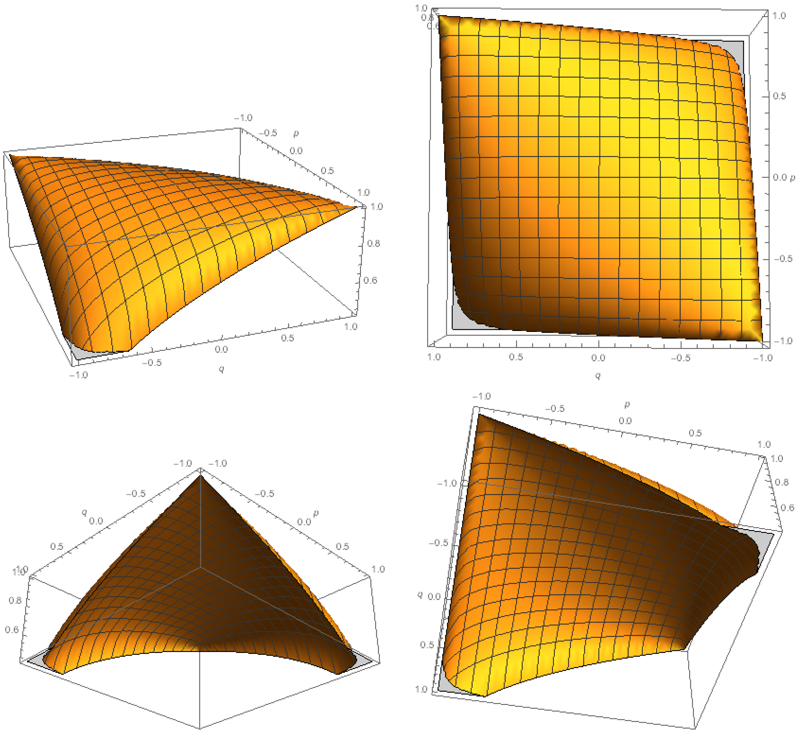
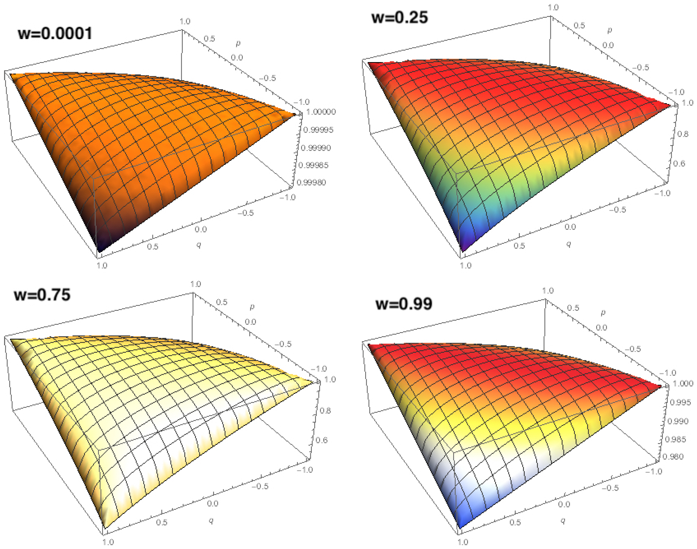
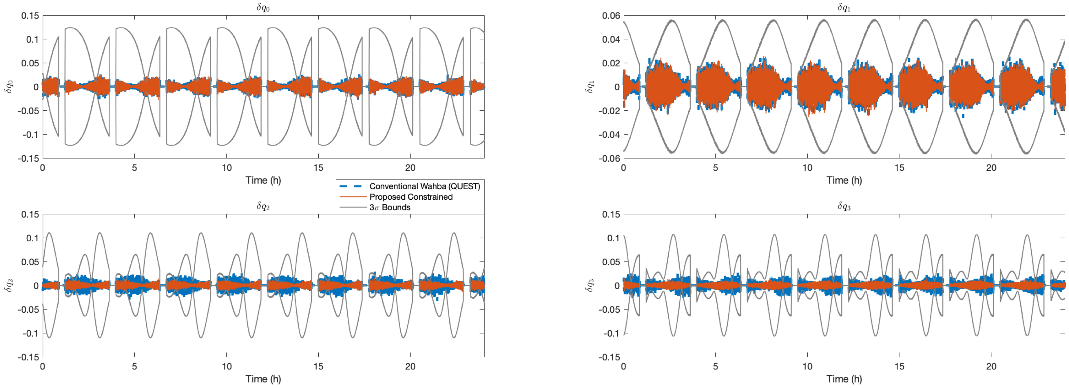
3.3. Error and Covariance Anlysis

Equation (1) is an ideal model for two-vector attitude determination without noises. The noise-corrupted model is expressed as follows
b 1 + e 1 = C ( r 1 + ε 1 ) b 2 + e 2 = C ( r 2 + ε 2 )
where e 1 , e 2 , ε 1 , and ε 2 are independent white Gaussian noise items with covariances of Σ b 1 , Σ b 2 , Σ r 1 , and Σ r 2 , respectively. Assume that for the true value K we have a corresponding true quaternion q with eigenvalue 1, such that
Kq = q
With noise perturbation, K is interfered with by δ K , also generating an eigenvector perturbation δ q , say
K + δ K q + δ q = q + δ q
Expanding it yields
Kq + δ Kq + K δ q + δ K δ q = q + δ q δ Kq + K δ q + δ K δ q = δ q δ Kq = ( K + δ K I ) δ q
As we also have det ( K + δ K I ) = 0 , the quaternion perturbation is derived by
( K + δ K I ) δ Kq = δ q
which produces the following quaternion difference [40],
δ q = I K δ K q
with
δ K = δ κ δ z T δ z δ B + δ B T δ κ I δ B = w b 1 ε 1 T + e 1 r 1 T + 1 w b 2 ε 2 T + e 2 r 2 T δ z = w b 1 × ε 1 + e 1 × r 1 + 1 w b 2 × ε 2 + e 2 × r 2 δ κ = w ε 1 T b 1 + r 1 T e 1 + 1 w ε 2 T b 2 + r 2 T e 2
The above error analysis is the standard approach for the Wahba’s solution using Davenport q-method. This error-analysis approach is presented to cope with the restriction of the unknown eigenvalues associated with the Davenport q-method. However, such results are also related to the selection of the weight w. Apparently, seen from Solution Equation (43), one may easily see that the obtained quaternion is free of w. This type of quaternion owns closed forms without high-order or highly nonlinear terms. Therefore for the proposed method, the error analysis can be performed easily using
δ q = 1 α 2 + β 2 + γ 2 + N 2 δ α , δ β , δ γ , δ N T + δ 1 α 2 + β 2 + γ 2 + N 2 α , β , γ , N T
with
δ 1 α 2 + β 2 + γ 2 + N 2 = α 2 + β 2 + γ 2 + N 2 3 2 α δ α + β δ β + γ δ γ + N δ N
and δ α , δ β , δ γ , and δ N can be computed directly from Equation (43).
Then, the covariance of the derived quaternion using first-order approximation is also straightforward, given by
Σ q = J Σ b 1 Σ b 2 Σ r 1 Σ r 2 J T
where the Jacobian J is
J = q b 1 T , b 2 T , r 1 T , r 2 T T

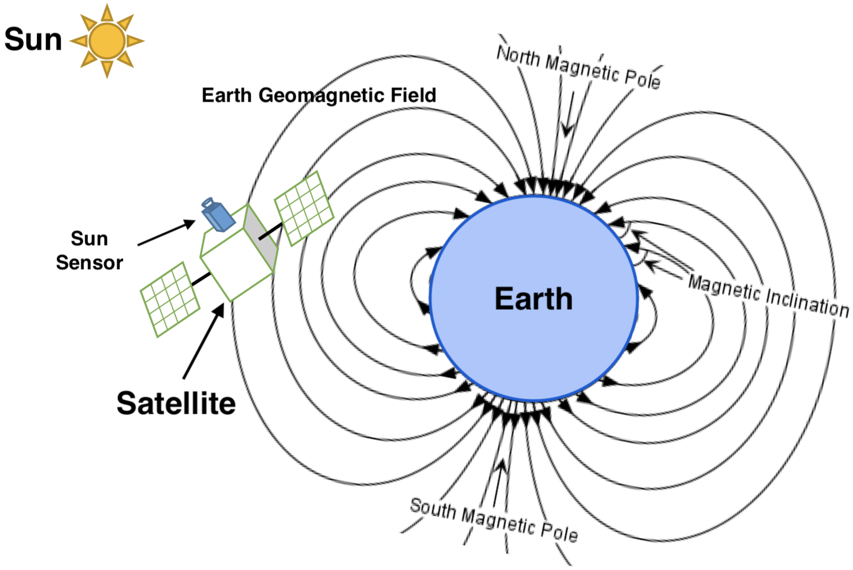
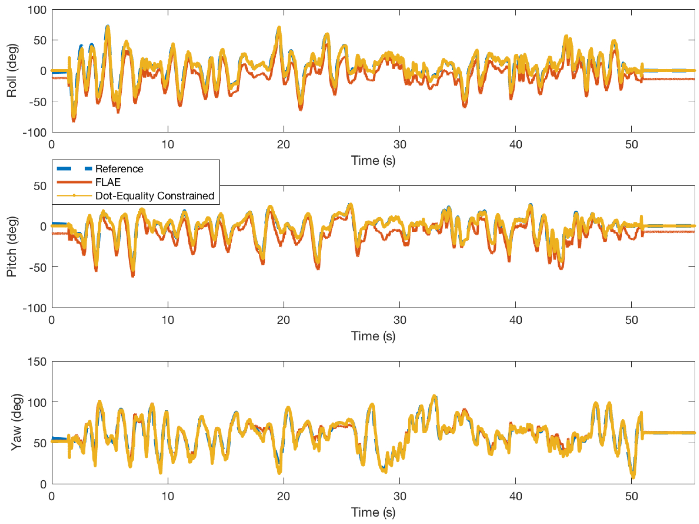
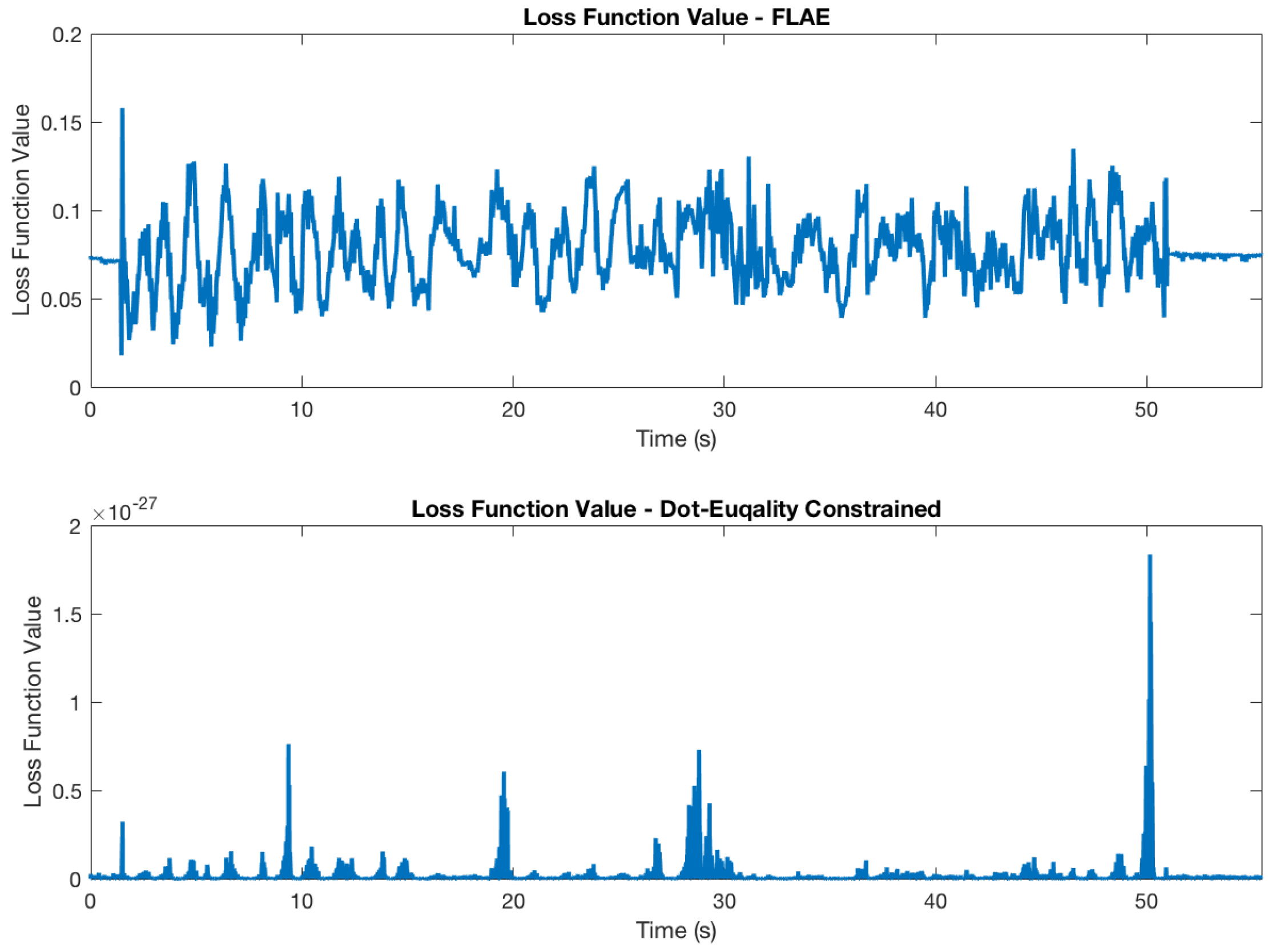
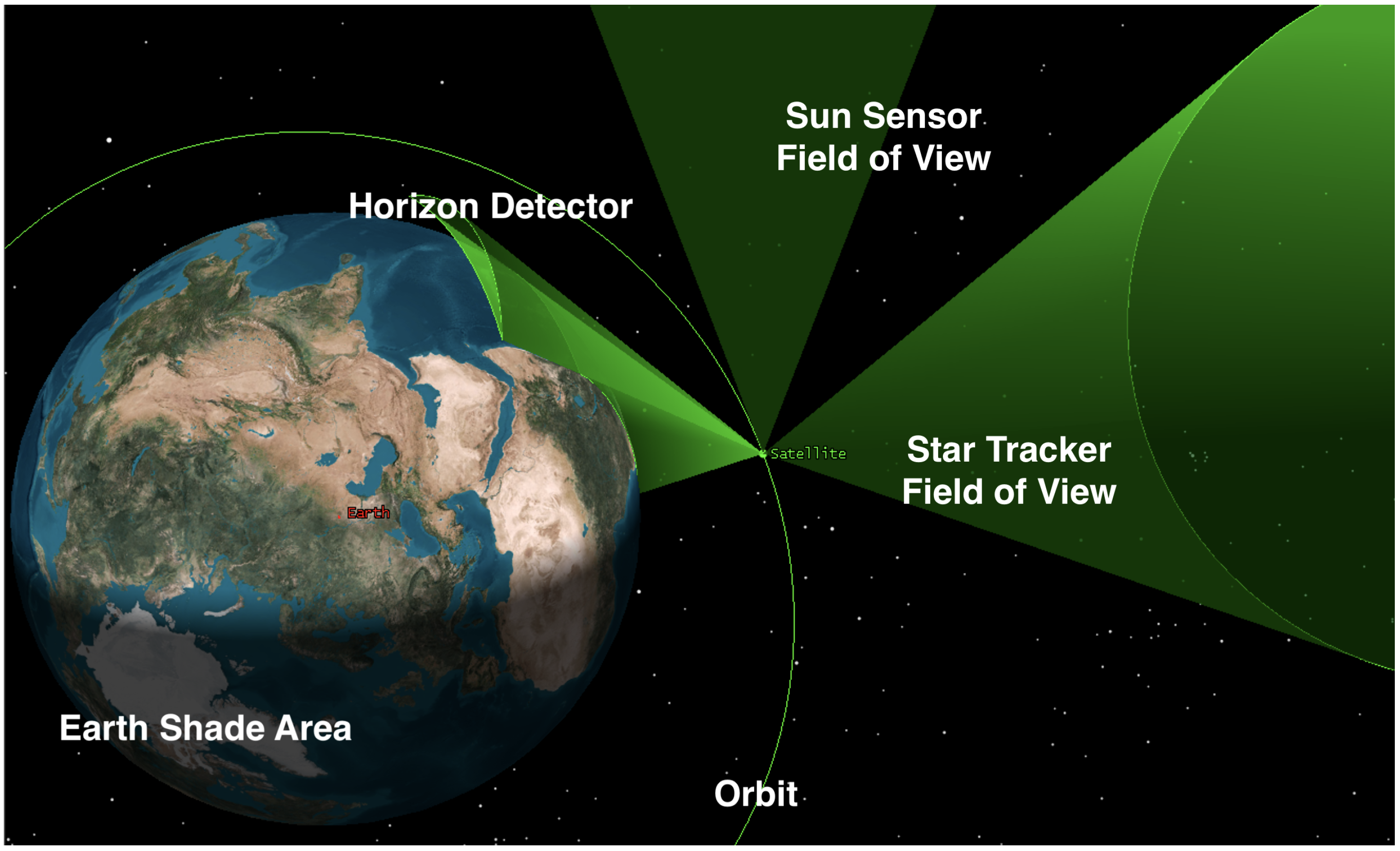
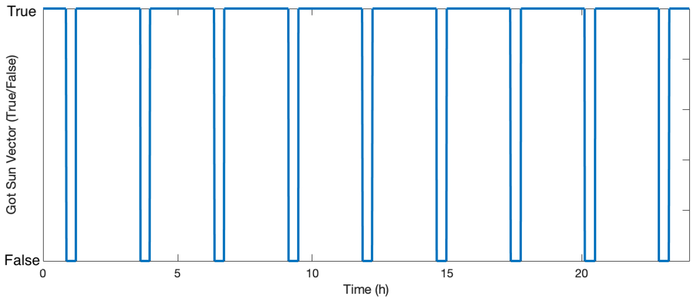
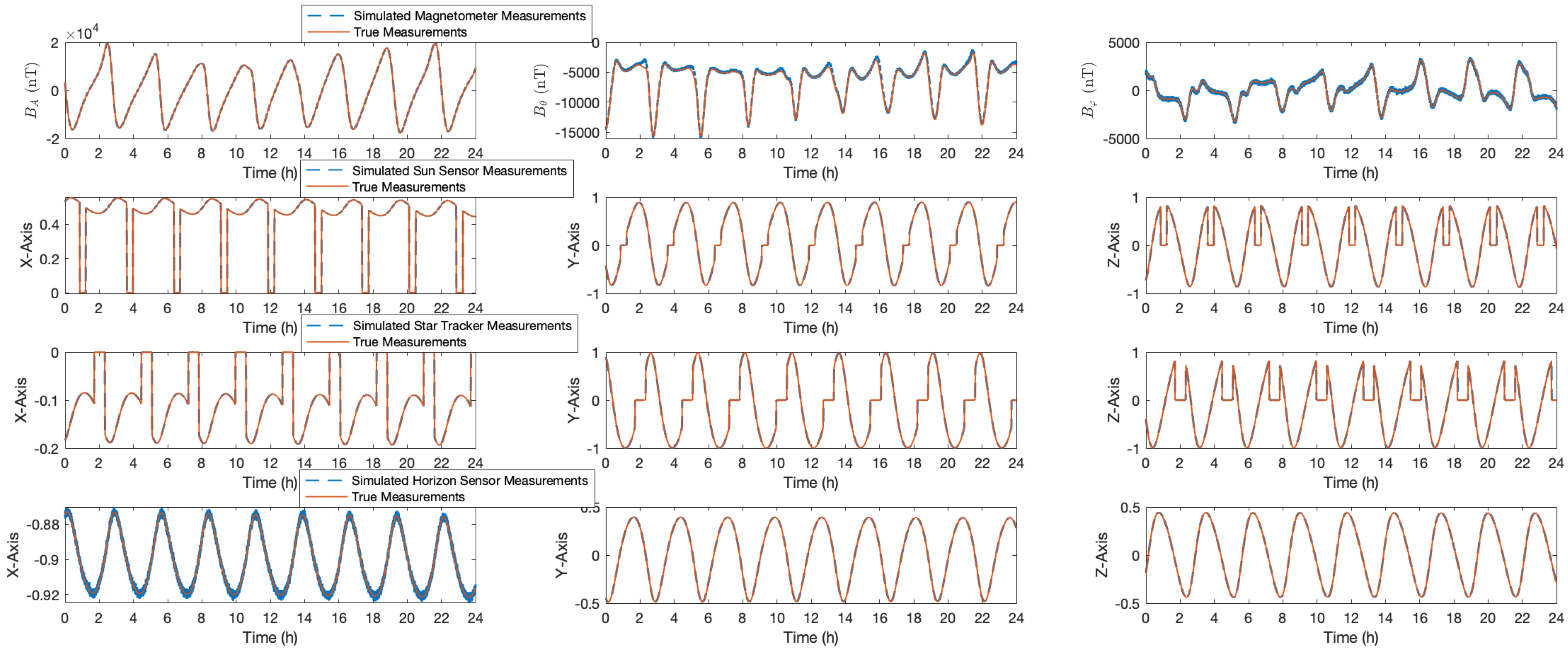
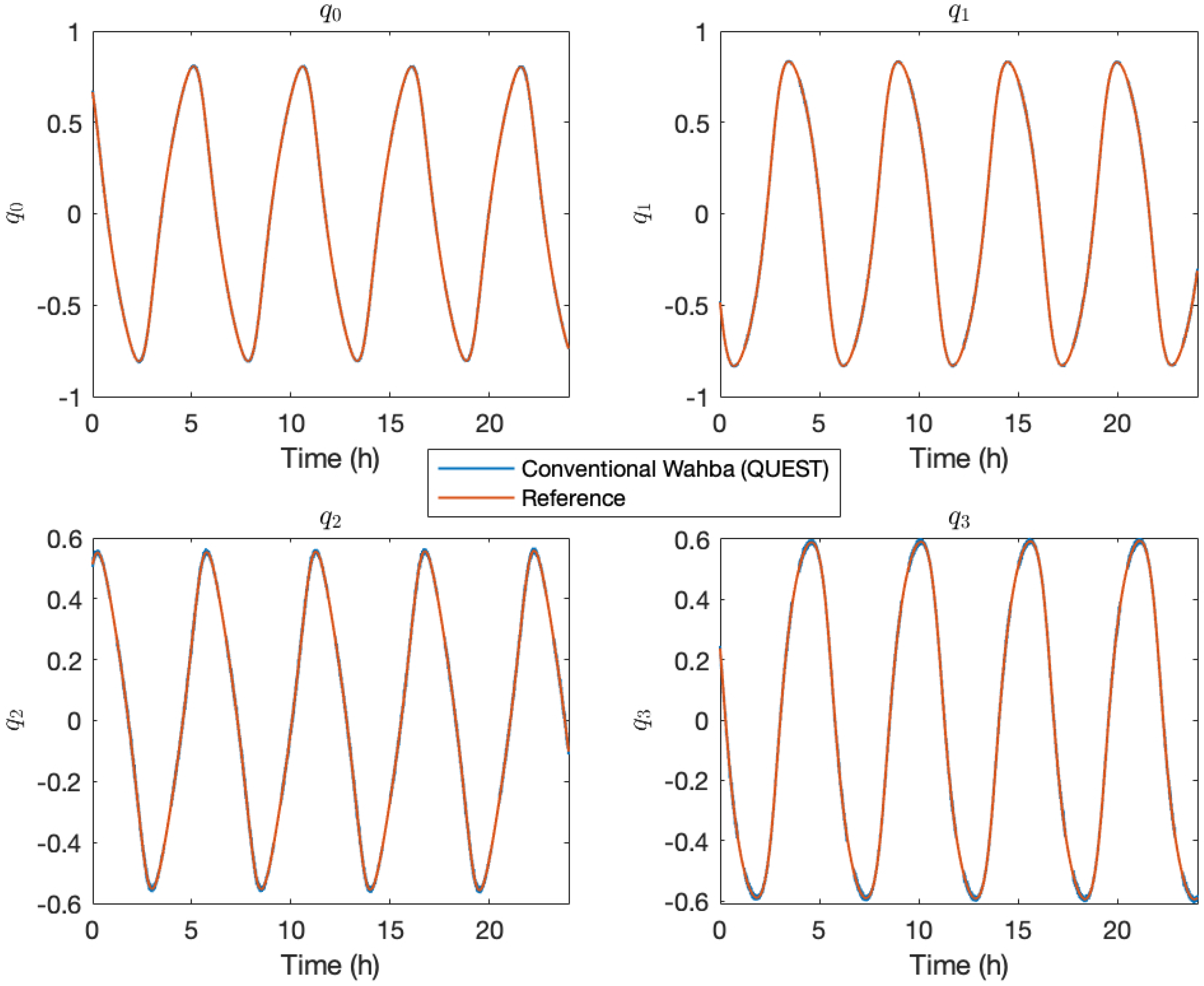
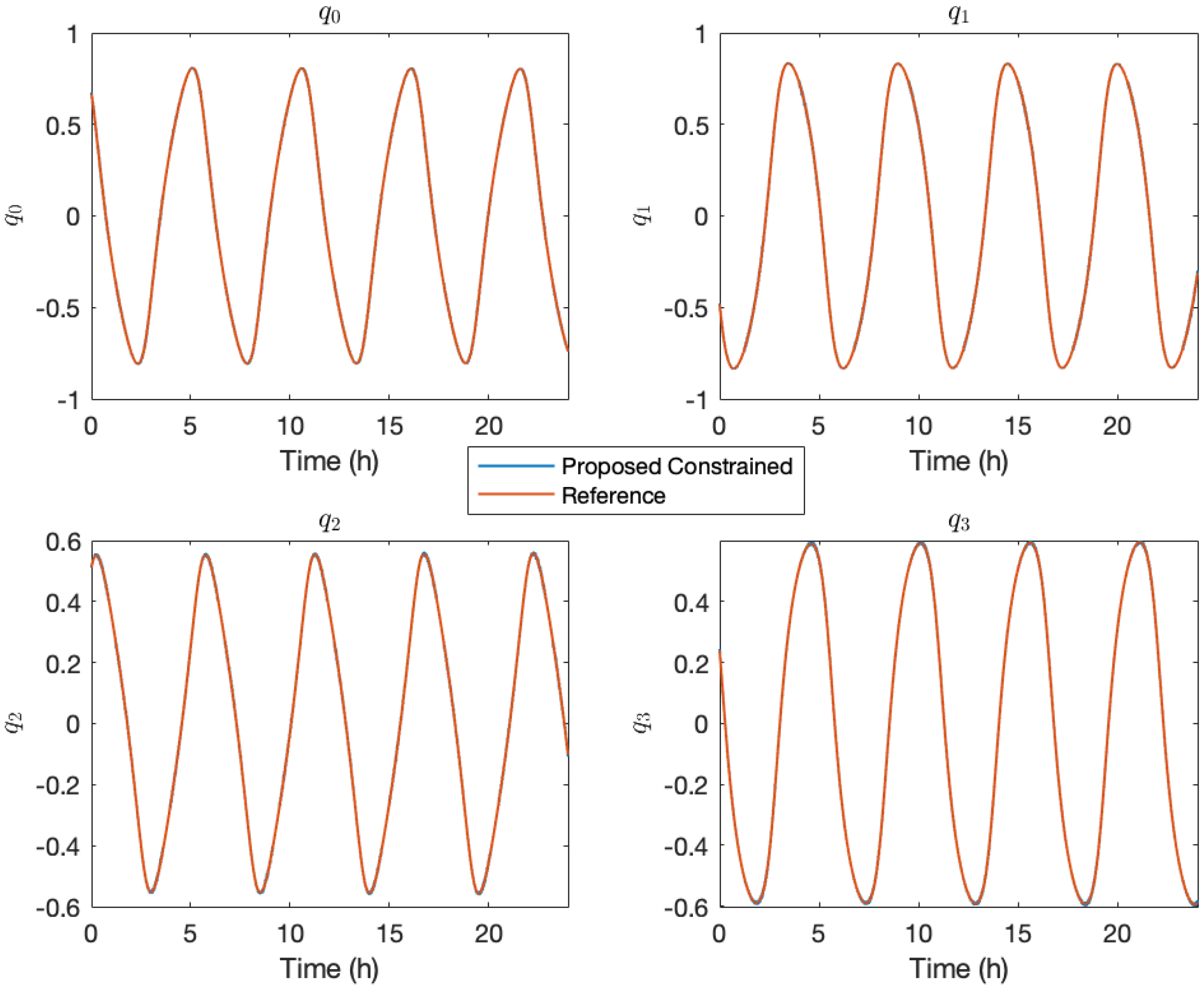
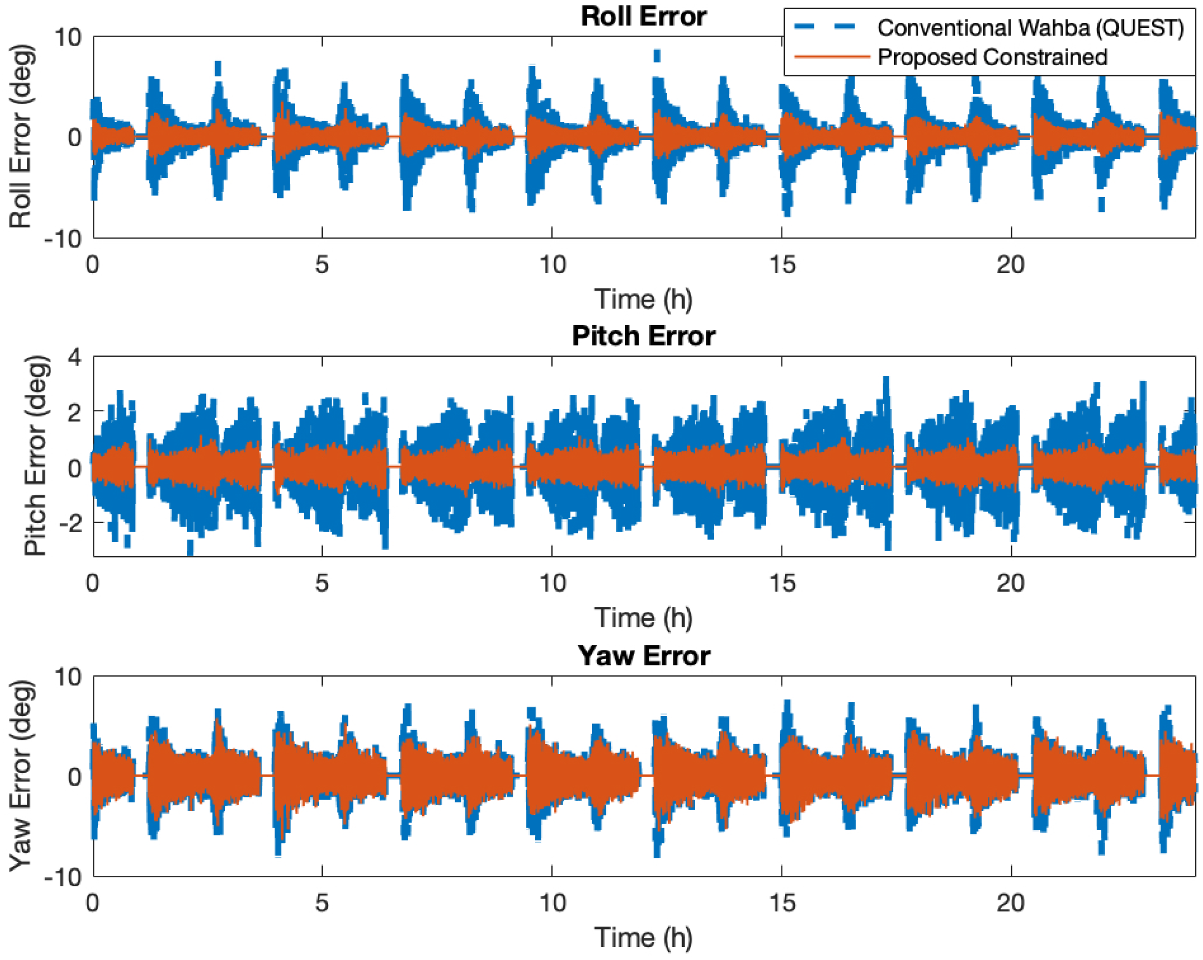
4. Applications: Attitude Determination from Horizon Sensor and Another Generalized Sensor

The derived theory can be applied to those problems in which some of the reference vectors are hard to be determined. In this section, we choose the system configuration with a horizon sensor and another generalized sensor for two-vector attitude determination. The horizon sensor can be either an infrared Nadir detector [41] or a camera-based horizon finder [42]. It estimates the horizontal Euler angles of the mounting object by tracking Nadir or analyzes the geometry of the camera-captured horizon. Also, we need to note that in near-ground static applications, accelerometers can be used for reconstruction of roll and pitch information and can also be treated as a kind of horizon sensor.
There are many other types of sensors for a horizon sensor to accompany. For instance, the attitude determination by means of accelerometer and magnetometer can be used for pedestrian navigation. The infrared Nadir detector together with Sun sensor or magnetometer can also provide accurate enough attitude determination results. Take the accelerometer–magnetometer case for example, the magnetic reference vector is usually time-varying with the position of the rigid body. This is because the Earth geomagnetic field can be described by the following potential [43].
U = A n = 1 k m = 1 n R e A n + 1 P n m ( cos θ ) ( g n m cos m φ + h n m sin m φ )
where A denotes the distance of the object to the Earth center; R e is the Earth radius; θ and φ are co-latitude and longitude, respectively; P n m is the associated Legendre function of degree m and order n; and g n m and h n m are Gaussian coefficients from global satellite geomagnetic measurements and are released in annual IGRF models. Then, the magnetic vector in the geodetic frame is the function of A , θ , and φ . The most common way to obtain such reference information is by looking up the table or directly computing the vector by spheric harmonic functions. However, when there is no source of position measurements (such as low-cost indoor smart wearables), it is very hard to obtain such information. A compromising way is to use the magnetic north rather than the true north provided by IGRF. Assuming that the accelerometer and magnetometer have their normalized vector measurements pairs as follows,
A b = a x , a y , a z T A r = 0 , 0 , 1 T , M b = m x , m y , m z T M r = m N , 0 , m D T
we can directly construct the magnetic reference vector by
A b · M b = A r · M r m D = a x m x + a y m y + a z m z
whereas another component can be determined by
m N = cos κ = 1 m D 2
where κ is the local dip angle [44]. From the derived results shown in last section, the quaternion calculated now only obtains roll, pitch from accelerometer, and yaw from magnetometer, respectively. The magnetometer does not influence the estimation of other two angles and neither does the accelerometer [28].
A record of accelerometer/magnetometer data along with reference angles are logged from the 3DM-GX3-25 attitude and heading reference system (AHRS). This AHRS module is attached to the data collection computer via the serial port with baudrate of 921600. The sampling frequency is set to 500 Hz. The motion has been generated using a human-operated inertial stabilized gimbal so that the motion in all axes will be produced. The motivation of using the accelerometer and magnetometer as an experimental object is that we would like to theoretically explain why attitude estimation can be conducted in a reference-free manner as presented in previous literatures [21,28,45,46,47]. Using MATLAB r2016b, we evaluate the attitude determination results in Figure 4. The related loss functions are plotted in Figure 5. The results in Figure 5 magnify the nonintuitive errors presented in Figure 4.
In this experiment, the weights between accelerometer and magnetometer are both 0.5 . The local magnetic reference vector of FLAE is set to M r = ( 0.9800 , 0 , 0.1989 ) T in the Northern Hemisphere. It is noticed from the figure that the roll and pitch angle determination has more observable differences than that of the proposed method between the true angles. This is because the roll and pitch angles used herein are not fully determined by the accelerometer but influenced by magnetometer as well. For the conventional Wahba’s problem, the two sensors both contribute to the observabilities of three Euler angles roll, pitch, and yaw. However, using the proposed method, we can separate these observabilities. Apart from the errors in the local magnetic reference vector during movement, the AHRS has been somewhat distorted by outer unknown electromagnetic disturbances. In such occasion, the non-yaw angles would contain evident differences with the reference values. If the proposed method behaves, the angles fit those from the reference instrument very well. The internal reason has been introduced before i.e., the roll and pitch angles are fully measured from the accelerometer while the yaw is only determined by the magnetometer. The loss function results also reflect this point. Coinciding with previous findings, the loss function values from the proposed method vary at the basic scale of 1 × 10 27 which is tiny enough to be considered as zero.
While for the more general case in which there are one horizon sensor and another sensor, using the results in Equation (43), we can give the analytical solution to such attitude determination problem by
q = 1 q ˜ 0 2 + q ˜ 1 2 + q ˜ 2 2 + q ˜ 3 2 q ˜ 0 , q ˜ 1 , q ˜ 2 , q ˜ 3 T q ˜ 0 = f x g y h x g x h y + f y g z f z h z + f z 2 1 h y q ˜ 1 = f x g x h z g z h x + f y g z h y g y h z f x g x + f y g y + f z f x h x f y h y + f z 2 1 1 h z q ˜ 2 = f y h x g z f z g x h z 1 + f x h y g z f z g y h z 1 q ˜ 3 = h x f y g y + f z 2 1 f y g x h y + f x f z h z g z
where
h b = ( h x , h y , h z ) T h r = ( 0 , 0 , 1 ) T g b = ( g x , g y , g z ) T g r = ( f x , f y , f z ) T
and h b and h r are vector observation pair for the horizon sensor in b and r frames, respectively, whereas g b and g r represent the same meaning for another generalized sensor.
Now, we simulate a mission for a satellite. Four sensors, including a star tracker, a horizon sensor, a Sun sensor, and a magnetometer, are employed (see Figure 6). Only the horizon sensor and Sun sensor are employed to compute the attitude in this section; the other sensors are used for generating high-resolution attitude reference information. All of the sensors presented in this simulation study are transformed into the J2000 Earth-Centered Interval (ECI) frame for attitude computation. The Sun vector can be computed straightforward according to historical astronomy ephemeris [48]. Given the Julian time T JD [49]:
T JD = 367 year 7 year + month + 9 12 4 + 275 month 9 + day + 1721013.5 + hour 24 + minute 1440 + second 86400
where is the downward floor operator, thus the normalized Sun vector g r can be determined by
U T 1 = T JD 2451545 36525 M s u n = 357.5277233 + 35999.05034 U T 1 γ e c l i p t i c = 280.4606184 + 36000.77005361 U T 1 + 1.914666471 sin π M s u n 180 + 0.918994643 sin 2 π M s u n 180 e s u n = 23.439291 0.0130042 U T 1 s x = cos ( π γ e c l i p t i c 180 ) s y = cos ( π e s u n 180 ) sin ( π γ e c l i p t i c 180 ) s z = sin ( π e s u n 180 ) sin ( π γ e c l i p t i c 180 ) g r = 1 s x 2 + s y 2 + s x 2 ( s x , s y , s z ) T
where M s u n denotes the Sun mean anomaly, γ e c l i p t i c is the ecliptic longitude of the Sun, and e s u n stands for the eccentricity of the Sun orbit.
The satellite motion is simulated by creating an orbit around the Earth with eccentricity of 0.15 and semimajor axis of 9966.14 km . The satellite attitude is generated with Nadir alignment subject to orbit normal constraint of 3 deg . The spacecraft attitude has been simulated through the following equation of angular momentum,
I ω ˙ + h ˙ + ω × ( I ω + h ) = u
where I denotes the inertia of spacecraft, ω is the angular rate, and h stands for the angular momentum driven by the control input u . The attitude model has been constructed via the 4-th Runge–Kutta method, and the control method used herein is a Propotional-Derivative (PD)-type control algorithm. The star tracker in this simulation points exactly to the Hipparcos 2 24608 star. The outer geomagnetic environment has the perturbation based on the Olson-Pfitzer field. The IGRF model for the magnetometer measurement in the local geodetic frame is expressed as follows.
B A , B θ , B φ T = U B A = n = 1 k R e A n + 2 ( n + 1 ) m = 0 n g n m cos m φ + h n m sin m φ P n m ( cos θ ) B θ = n = 1 k R e A n + 2 m = 0 n g n m cos m φ + h n m sin m φ P n m ( cos θ ) θ B φ = 1 sin θ n = 1 k R e A n + 2 m = 0 n m g n m sin m φ + h n m cos m φ P n m ( cos θ )
The Sun sensor not always work, as there may be an area of shade due to the Earth’s positioning during flight that prohibits Sun detection. The simulation is run for 1 single day from 1 March 2019 04:00:00.000 to 2 March 2019 04:00:00.000. The available solar luminance is indicated in Figure 7. The Sun sensor has accuracy of 20 arcsec and for horizon sensor that would be 1.5 arcmin . The sensor noises are simulated to be additive and subject to the Gaussian distribution. When the spacecraft is in the Earth shade area, we do not compute the attitude since only one vector observation pair does not have enough observability for three-axis attitude determination.
The raw measurements of the four attitude sensors are presented in Figure 8 where the measured values of Sun sensor, star tracker, and the horizon sensor are presented in the normalized form.
Using the representative QUEST solver for conventional Wahba’s problem, we show the comparison with the proposed method. Figure 9 and Figure 10 show the results from QUEST and the proposed algorithm, respectively.
The results show that both methods are efficient for attitude determination. However, since the proposed method separates the effects of the horizon sensor and Sun sensor, the attitude error covariance has a smaller scale than QUEST. The quaternion error responses of QUEST and the proposed algorithm are shown in Figure 11. In Figure 11, the 3 σ bounds are also presented using the square roots of the diagonal elements of the computed quaternion error covariances. Corresponding Euler angle errors are shown in Figure 12. The QUEST has the root-mean-squared error (RMSE) attitude accuracy of 5.12 deg on roll, 2.34 deg on pitch, and 4.06 deg on yaw. The proposed method has advantages on roll and pitch and has RMSE attitude accuracy of 2.93 deg on roll, 1.01 deg on pitch, and 3.82 deg on yaw. The proposed method can make the attitude propagation from sensors independently and thus when emergency occurs the engineers may be also easier to separate the faults and will find out the sensor failures much faster; that is, if the horizon sensor has exceptions, only roll and pitch will be affected, whereas the Sun sensor encounters faults only if yaw can be influenced.

5. Conclusions

In this paper, we revisit the problem of two-vector attitude determination, which is based on the theory of Markley [25]. A novel dot product equality constraint is proposed to further support the conventional optimization. The quaternion solutions and covariance analysis are also obtained for implementation on chips. By virtue of the equality constraint, the derived quaternion result can separate sensor effects for independent attitude angle observabilities. The derived quaternion solution is not as neat as that provided in the work by the authors of [26], but it provides another perspective without matrix orthonormalization. An application on the attitude determination from the horizon sensor and another generalized sensor illustrates that the proposed method is effective and accurate. It has also been tested smaller covariance scales in the presented simulation study for spacecraft attitude determination. Future works should be devoted to invoke more vector observation pairs for generalized attitude determination tasks. Also, according to the independent angle separation functionality of the proposed work, it may be used for flexible sensor calibration in further studies.

Author Contributions

J.W. proposed the main theory; S.S. conducted experimental validations.

Funding

This research was supported by National Natural Science Foundation of China under the grant of No. 61803383.

Acknowledgments

The authors would like to thank H. E. Soken from the TUBITAK Space Technologies Research Institute, Turkey, for invitation of submission to this special issue. We also would like to thank F. L. Markley, from NASA Goddard Space Flight Center, for his constructive suggestions to the revision of this paper.

Conflicts of Interest

The authors declare no conflicts of interest.

References

  1. Gui, H.; Jin, L.; Xu, S. Attitude maneuver control of a two-wheeled spacecraft with bounded wheel speeds. Acta Astronaut. 2013, 88, 98–107. [Google Scholar] [CrossRef]
  2. Mortari, D.; Singla, P. Optimal cones intersection technique. Acta Astronaut. 2006, 59, 474–482. [Google Scholar] [CrossRef]
  3. de Ruiter, A.H.J.; Tran, L.; Kumar, B.S.; Muntyanov, A. Sun Vector–Based Attitude Determination of Passively Magnetically Stabilized Spacecraft. AIAA J. Guid. Control Dyn. 2016, 39, 1551–1562. [Google Scholar] [CrossRef]
  4. Mumtaz, R.; Palmer, P. Attitude determination by exploiting geometric distortions in stereo images of DMC camera. IEEE Trans. Aerosp. Elec. Syst. 2013, 49, 1601–1625. [Google Scholar] [CrossRef]
  5. Pham, M.D.; Low, K.S.; Goh, S.T.; Chen, S. Gain-Scheduled Extended Kalman Filter for Nanosatellite Attitude Determination System. IEEE Trans. Aerosp. Elec. Syst. 2015, 51, 1017–1028. [Google Scholar] [CrossRef]
  6. Saez, A.B.; Quero, J.M.; Jerez, M.A. Earth Sensor Based on Thermopile Detectors for Satellite Attitude Determination. IEEE Sensors J. 2016, 16, 2260–2271. [Google Scholar] [CrossRef]
  7. Mahony, R.; Hamel, T.; Pflimlin, J.M. Nonlinear complementary filters on the special orthogonal group. IEEE Trans. Autom. Control 2008, 53, 1203–1218. [Google Scholar] [CrossRef]
  8. Wang, M.; Tayebi, A. Hybrid Pose and Velocity-bias Estimation on SE(3) Using Inertial and Landmark Measurements. IEEE Trans. Autom. Control 2018, 64, 3399–3406. [Google Scholar] [CrossRef]
  9. Zhou, Z.; Li, Y.; Liu, J.; Li, G. Equality constrained robust measurement fusion for adaptive kalman-filter-based heterogeneous multi-sensor navigation. IEEE Trans. Aerosp. Electron. Syst. 2013, 49, 2146–2157. [Google Scholar] [CrossRef]
  10. Zhou, Z.; Li, Y.; Zhang, J.; Rizos, C. Integrated Navigation System for a Low-Cost Quadrotor Aerial Vehicle in the Presence of Rotor Influences. J. Survey. Eng. 2017, 143, 05016006. [Google Scholar] [CrossRef]
  11. Wahba, G. A Least Squares Estimate of Satellite Attitude. SIAM Rev. 1965, 7, 409. [Google Scholar] [CrossRef]
  12. Shuster, M.D.; Oh, S.D. Three-axis attitude determination from vector observations. AIAA J. Guid. Control Dyn. 1981, 4, 70–77. [Google Scholar] [CrossRef]
  13. Markley, F.L. Attitude Determination using Vector Observations and the Singular Value Decomposition. J. Astronaut. Sci. 1988, 36, 245–258. [Google Scholar]
  14. Mortari, D. EULER-q algorithm for attitude determination from vector observations. AIAA J. Guid. Control Dyn. 1998, 21, 328–334. [Google Scholar] [CrossRef]
  15. Patera, R.P. Attitude estimation based on observation vector inertia. Adv. Space Res. 2018, 62, 383–397. [Google Scholar] [CrossRef]
  16. Yang, Y. Attitude determination using Newton’s method on Riemannian manifold. Proc. IMechE Part G J. Aerosp. Eng. 2015, 229, 2737–2742. [Google Scholar] [CrossRef]
  17. Zhou, Z.; Wu, J.; Wang, J.; Fourati, H. Optimal, Recursive and Sub-optimal Linear Solutions to Attitude Determination from Vector Observations for GNSS/Accelerometer/Magnetometer Orientation Measurement. Remote Sens. 2018, 10, 377. [Google Scholar] [CrossRef]
  18. Wu, J.; Zhou, Z.; Fourati, H.; Li, R.; Liu, M. Generalized Linear Quaternion Complementary Filter for Attitude Estimation from Multi-Sensor Observations: An Optimization Approach. IEEE Trans. Auto. Sci. Eng. 2019, 16, 1330–1343. [Google Scholar] [CrossRef]
  19. Marins, J.; Yun, X.; Bachmann, E.; McGhee, R.; Zyda, M. An extended Kalman filter for quaternion-based orientation estimation using MARG sensors. In Proceedings of the 2001 IEEE/RSJ International Conference on Intelligent Robots and Systems, Maui, HI, USA, 29 October–3 November 2001; Volume 4. [Google Scholar]
  20. Fourati, H.; Manamanni, N.; Afilal, L.; Handrich, Y. Complementary Observer for Body Segments Motion Capturing by Inertial and Magnetic Sensors. IEEE/ASME Trans. Mech. 2014, 19, 149–157. [Google Scholar] [CrossRef]
  21. Yun, X.; Bachmann, E.R.; McGhee, R.B. A simplified quaternion-based algorithm for orientation estimation from earth gravity and magnetic field measurements. IEEE Trans. Instrum. Meas. 2008, 57, 638–650. [Google Scholar] [CrossRef]
  22. Bar-Itzhack, I.Y.; Harman, R.R. Optimized TRIAD Algorithm for Attitude Determination. AIAA J. Guid. Control Dyn. 1997, 20, 208–211. [Google Scholar] [CrossRef] [Green Version]
  23. Abdelrahman, M.; Park, S.Y. Simultaneous spacecraft attitude and orbit estimation using magnetic field vector measurements. Aerosp. Sci. Technol. 2011, 15, 653–669. [Google Scholar] [CrossRef]
  24. Psiaki, M.L. Autonomous Low-Earth-Orbit Determination from Magnetometer and Sun Sensor Data. AIAA J. Guid. Control Dyn. 1999, 22, 296–304. [Google Scholar] [CrossRef]
  25. Markley, F.L. Fast Quaternion Attitude Estimation from Two Vector Measurements. AIAA J. Guid. Control Dyn. 2002, 25, 411–414. [Google Scholar] [CrossRef] [Green Version]
  26. Markley, F.L. Optimal Attitude Matrix from Two Vector Measurements. AIAA J. Guid. Control Dyn. 2008, 31, 765–768. [Google Scholar] [CrossRef]
  27. Wiegand, M. Autonomous Satellite Navigation via Kalman Filtering of Magnetometer Data. Acta Astronaut. 1996, 38, 395–403. [Google Scholar] [CrossRef]
  28. Wu, J.; Zhou, Z.; Fourati, H.; Cheng, Y. A Super Fast Attitude Determination Algorithm for Consumer-Level Accelerometer and Magnetometer. IEEE Trans. Consum. Elect. 2018, 64, 375–381. [Google Scholar] [CrossRef]
  29. de Ruiter, A.H.J.; Forbes, J.R. Discrete-Time SO(n)-Constrained Kalman Filtering. AIAA J. Guid. Control Dyn. 2017, 40, 28–37. [Google Scholar] [CrossRef]
  30. de Ruiter, A.H.J. Quadratically Constrained Least Squares with Aerospace Applications. AIAA J. Guid. Control Dyn. 2016, 39, 487–497. [Google Scholar] [CrossRef] [Green Version]
  31. Zanetti, R.; Majji, M.; Bishop, R.H.; Mortari, D. Norm-Constrained Kalman Filtering. AIAA J. Guid. Control Dyn. 2009, 32, 1458–1465. [Google Scholar] [CrossRef]
  32. Crassidis, J.L.; Markley, F.L.; Cheng, Y. Survey of Nonlinear Attitude Estimation Methods. AIAA J. Guid. Control Dyn. 2007, 30, 12–28. [Google Scholar] [CrossRef]
  33. Davenport, P.B. A Vector Approach to the Algebra of Rotations with Applications; Technical Report August; NASA: Washington, DC, USA, 1968. [Google Scholar]
  34. Mortari, D. ESOQ-2 single-point algorithm for fast optimal spacecraft attitude determination. Adv. Astronaut. Sci. 1997, 95 Pt 2, 817–825. [Google Scholar]
  35. Yang, Y.; Zhou, Z. An analytic solution to Wahbas problem. Aerosp. Sci. Technol. 2013, 30, 46–49. [Google Scholar] [CrossRef]
  36. Wu, J.; Zhou, Z.; Gao, B.; Li, R.; Cheng, Y.; Fourati, H. Fast Linear Quaternion Attitude Estimator Using Vector Observations. IEEE Trans. Auto. Sci. Eng. 2018, 15, 307–319. [Google Scholar] [CrossRef]
  37. Wu, J. Optimal Continuous Unit Quaternions from Rotation Matrices. AIAA J. Guid. Control. Dyn. 2019, 42, 919–922. [Google Scholar] [CrossRef]
  38. Barfoot, T.; Forbes, J.R.; Furgale, P.T. Pose estimation using linearized rotations and quaternion algebra. Acta Astronaut. 2011, 68, 101–112. [Google Scholar] [CrossRef]
  39. Wu, J. Real-time Magnetometer Disturbance Estimation via Online Nonlinear Programming. IEEE Sens. J. 2019, 19, 4405–4411. [Google Scholar] [CrossRef]
  40. Chang, G.; Xu, T.; Wang, Q. Error analysis of Davenport’s q method. Automatica 2017, 75, 217–220. [Google Scholar] [CrossRef]
  41. Nguyen, T.; Cahoy, K.; Marinan, A. Attitude Determination for Small Satellites with Infrared Earth Horizon Sensors. AIAA J. Spacecr. Rocket. 2018, 55, 1466–1475. [Google Scholar] [CrossRef]
  42. Carrio, A.; Bavle, H.; Campoy, P. Attitude estimation using horizon detection in thermal images. Int. J. Micro Air Veh. 2018, 10, 352–361. [Google Scholar] [CrossRef] [Green Version]
  43. Abdelrahman, M.; Park, S.Y. Integrated attitude determination and control system via magnetic measurements and actuation. Acta Astronaut. 2011, 69, 168–185. [Google Scholar] [CrossRef] [Green Version]
  44. Sabatini, A.M. Quaternion-based extended Kalman filter for determining orientation by inertial and magnetic sensing. IEEE Trans. Biomed. Eng. 2006, 53, 1346–1356. [Google Scholar] [CrossRef] [PubMed]
  45. Valenti, R.G.; Dryanovski, I.; Xiao, J. A Linear Kalman Filter for MARG Orientation Estimation Using the Algebraic Quaternion Algorithm. IEEE Trans. Instrum. Meas. 2016, 65, 467–481. [Google Scholar] [CrossRef]
  46. Wu, J.; Zhou, Z.; Chen, J.; Fourati, H.; Li, R. Fast Complementary Filter for Attitude Estimation Using Low-Cost MARG Sensors. IEEE Sens. J. 2016, 16, 6997–7007. [Google Scholar] [CrossRef]
  47. Wu, J.; Wang, T.; Zhou, Z.; Yin, H.; Li, R. Analytic accelerometer-magnetometer attitude determination without reference information. Int. J. Micro Air Veh. 2019, 10, 318–329. [Google Scholar] [CrossRef]
  48. Furgale, P.; Enright, J.; Barfoot, T. Sun sensor navigation for planetary rovers: Theory and field testing. IEEE Trans. Aerosp. Elec. Syst. 2011, 47, 1631–1647. [Google Scholar] [CrossRef]
  49. Hajiyev, C.; Cilden, D.; Somov, Y. Gyro-free attitude and rate estimation for a small satellite using SVD and EKF. Aerosp. Sci. Technol. 2016, 55, 324–331. [Google Scholar] [CrossRef]
Figure 1. Satellite attitude determination system using observed Sun vector and geomagnetic sensing.
Aerospace 06 00102 g001
Figure 2. The plot of eigenvalue with p , q varying from 1 to 1, where w = 0.5 .
Aerospace 06 00102 g002

Figure 3. The plot of eigenvalue with p , q varying from 1 to 1, where w varies from 0.0001 to 0.99 .
Aerospace 06 00102 g003

Figure 4. Attitude determination results using the FLAE and proposed dot equality constrained method.
Aerospace 06 00102 g004
Figure 5. Loss function values from the FLAE and proposed dot equality constrained method.
Aerospace 06 00102 g005
Figure 6. The simulated spacecraft mission with horizon detector, Sun sensor, star tracker, and magnetometer. The magnetometer is installed in the interior part of the satellite and is invisible in the current image.
Aerospace 06 00102 g006
Figure 7. The Sun luminance indicator.
Aerospace 06 00102 g007
Figure 8. Raw measurements from various sensors.
Aerospace 06 00102 g008
Figure 9. The quaternion determination from QUEST.
Aerospace 06 00102 g009
Figure 10. The quaternion determination from the proposed method.
Aerospace 06 00102 g010
Figure 11. The quaternion accuracy comparison subject to input noises.
Aerospace 06 00102 g011
Figure 12. The attitude accuracy comparison subject to input noises.
Aerospace 06 00102 g012

