Trajectory Optimization of Extended Formation Flights for Commercial Aviation

Abstract

This paper presents a trajectory optimization study that has been conducted using a recently developed tool for the synthesis and analysis of extended flight formations of long-haul commercial aircraft, with the aim to minimize overall fuel consumption. In extended flight formations, trailing aircraft can attain an appreciable reduction in induced drag and associated reduction in fuel burn by flying in the upwash of the lead aircraft’s wake. In the present study, a previously developed multi-phase optimal control (MOC) framework for the synthesis of two-ship flight formations has been extended to include the assembly of three-ship flight formations. Using the extended tool, various numerical experiments have been conducted in relation to the assembly of two-ship and three-ship flight formations in long-haul operations across the North-Atlantic Ocean. Additionally, numerical experiments have been carried out to examine the impact of wind fields on the synthesis and performance of flight formations. Additionally, a parametric investigation has been conducted to assess the sensitivity of the solutions with respect to the degree of the induced drag reduction that might be attained by the trailing aircraft in a formation. The results of the various numerical experiments reveal that formation flight can result in appreciable reductions in fuel burn in comparison to flying solo—particularly when larger formation strings are permitted.

1. Introduction

Over the past two decades, a variety of numerical and experimental studies that have been carried out clearly reveal the potential of extended formation flight in considerably reducing fuel costs of long-haul commercial airline operations [1,2,3,4,5,6]. Although within an “extended” flight formation, the participating aircraft are relatively widely spaced in a longitudinal sense (i.e., 5–40 wingspans), trailing aircraft can still attain a significant reduction in induced drag by flying in the upwash of the lead aircraft’s wake, provided they are able to maintain the “sweet spot”—i.e., the most optimal (lateral and vertical) location relative to the lead aircraft. The sweet spot in terms of the lateral and vertical locations is limited to a radius smaller than 10% of the wingspan [7].

Initial research on formation flight was primarily focused on assessing the aerodynamic benefits in terms of induced drag reduction. Indeed, a wide variety of research studies—ranging from numerical aerodynamic performance predictions to wind-tunnel experiments and flight trials—have been conducted to quantify the potential aerodynamic benefits of extended formation flight [7,8,9,10,11,12,13]. A survey of the literature on this topic shows a fairly large spread of claimed performance benefits, indicating a reduction in induced drag of the trailing aircraft anywhere between 10% and 70% [7,8,9,10,11,12,13]. Moreover, the aerodynamic performance of trailing aircraft in a flight formation is highly dependent on the aircraft types/sizes in the formation, the number of aircraft in the formation string, and the formation flight geometry (i.e., relative aircraft spacing in three dimensions). With respect to the latter issue, the study presented in [7] clearly demonstrates the importance of precise lateral positioning of aircraft in a formation, with 50% of drag savings being lost if aircraft were unable to maintain their relative lateral position to within at least one tenth of a wingspan. The selected formation flight configuration (i.e., Echelon formation, V formation or inverted V formation) for formations involving more than two aircraft has been shown to have significant influence on the induced drag reduction benefits that can be attained.

In addition to aerodynamic performance prediction, there are several other key areas on which previous research on (extended) formation flight has focused. Significant research has, e.g., been devoted to the development of station keeping autopilots that enable formations to stay in the optimal position (the “sweet spot”) relative to each other [6]. Another key area relates to the planning and organization of flight formations on a network-wide scale [14,15,16,17]. Most studies addressing the planning and organization of flight formations often rely on a “bi-level” (or, “two-stage”) approach. In the first stage of this approach, the so-called routing/mission design problem is addressed. More specifically, in the routing/mission design problem, a formation is assembled based on a candidate set of typically two or three long-haul city-pair flights. Solving the routing/mission problem essentially boils down to finding the best location of the joining and splitting points of the formation and by establishing the associated fuel-optimal speed/altitude profiles. The second level/stage then essentially deals with the question “who flies with who”, attempting to optimize the network performance by selecting the most favorable subset of (two-ship and three-ship) formations and solo missions given the complete set of all possible formation flight options. Since a large number of formation options need to be explored for a network of realistic size, a computationally efficient optimization approach is called for in the first stage. For this reason, most bi-level approaches have relied on low-fidelity aircraft models for routing and mission design [16]. However, these low fidelity performance models do generally and unfortunately not produce very accurate results, and are rarely capable of handling real-world complications such as schedule delays and wind/weather influences.

Surprisingly, the development of higher-fidelity mission design optimization models—capable of handling real-world complications—has received very little attention within the research community to date. Only recently a study appeared that describes the development of a multi-phase optimal control (MOC) framework for the synthesis of two-ship formation flight missions, based on a high-fidelity point-mass model [18]. The main benefit of using a MOC formulation for the two-ship mission design problem is that it allows the simultaneous optimization of the single two-ship formation flight leg, and the four solo flights legs that link the origin airports to the joining point and the destination airports to the splitting point. In [18], the effectiveness of a multi-phase trajectory optimization (formation flight mission design) tool is demonstrated in a case study related to the assembly of two-ship formation flights across the North-Atlantic Ocean in the absence of wind. The results presented in this study not only confirm that formation flight can indeed result in appreciable fuel burn savings, but additionally reveals some very interesting characteristic features of the resulting formation flight trajectories that were not identified before.

In this study, the original MOC framework conceived in [18] is extended to permit the assembly of three-ship flight formations. As in [18], the effectiveness of the enhanced optimization framework is demonstrated in a transatlantic traversing scenario. An additional aspect addressed in the current study is the assessment of the influence of wind fields on formation flight performance and trajectory shaping. Finally, in view of the widely ranging estimates regarding the degree of (induced) drag reduction that can be attained in a flight formation, a sensitivity study is conducted to determine the differences in fuel burn and flight times that result from applying different levels of induced drag reduction for the trailing aircraft in a formation.

2. Trajectory Optimization Formulation

2.1. Trajectory Modelling

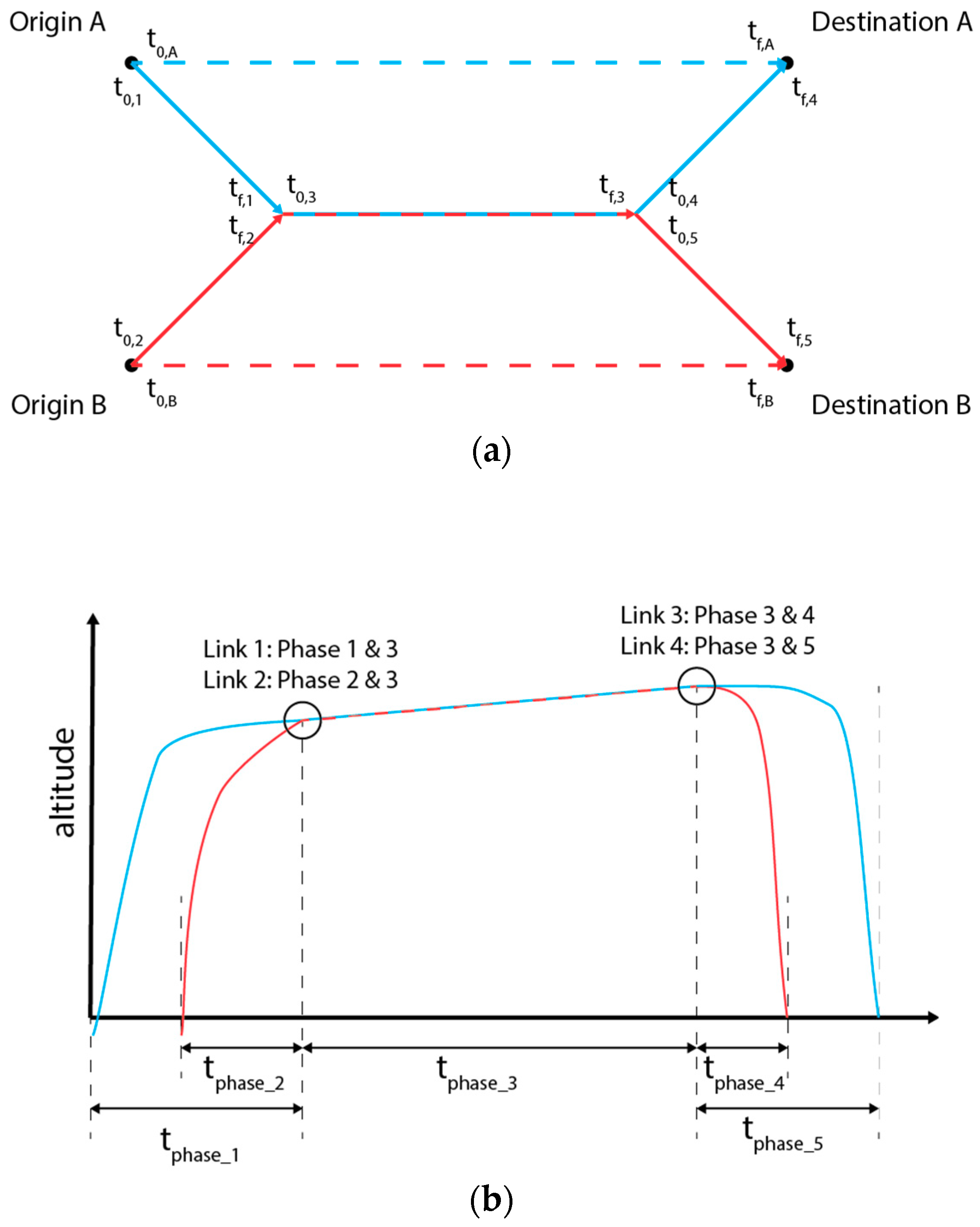
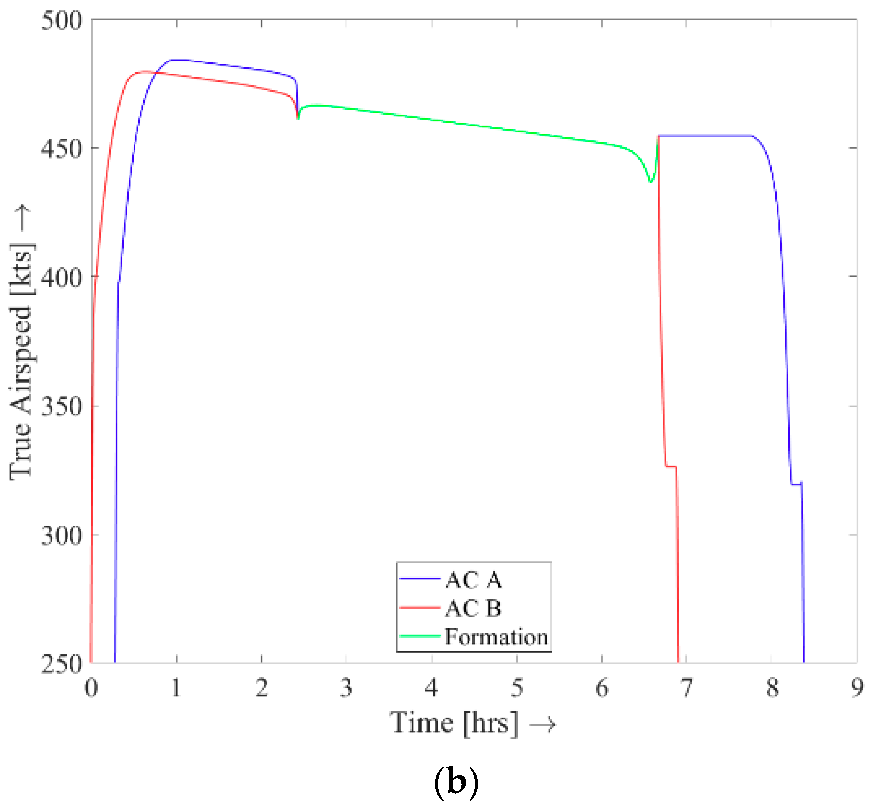
2.1.1. Two-Ship Formation Flight

The aim of this study is to optimize the trajectories in a three-dimensional space with respect to fuel consumption in the presence of wind for both two-ship and three-ship aircraft flight formations. In this subsection, the assembly of two-ship formations is considered in the context of a MOC formulation.

Figure 1a illustrates the multi-phase geometry pertaining to the two-ship formation assembly problem. In Figure 1a, two airline (solo) flights, labelled A and B, respectively, are scheduled to depart from two neighbouring origin airports towards two destination airports that are closely located as well. The departure times of the two city-pair (solo) flights are denoted as t_0,A and t_0,B, respectively, while the aircraft arrive at their destinations at t_f,A and t_f,B, respectively. As illustrated in Figure 1, the two-ship formation multi-phase assembly problem is modelled using five linked stages. The first two stages connect the two departing flights to the joining point, after which the actual formation flight is commenced (stage 3). The initial times for stages 1 and 2 are set equal to the departure times of the solo flights, i.e., t_0,1 = t_0,A and t_0,2 = t_0,B. To achieve rendezvous at the joining point, it is enforced that at the end of stages 1 and 2, t_f,1 = t_f,2 = t_rendezvous = t_0,3.

In Figure 1b, the formation assembly process in the vertical plane is schematically illustrated. The entry and exit points of the terminal manoeuvring area (TMA)—located at an altitude of 10,000 ft Above Ground Level—are taken as the initial and final points of the trajectories in this study.

It needs to be mentioned that in the employed multi-phase formulation the two considered aircraft are always forced to join in a formation—even when flying the city-pairs in solo flights is more favorable. For this reason, the optimization framework assesses not only the optimal performance of a formation flight, but also the performance of the two origin/destination (great circle) trajectories flown solo. This allows assessing under which conditions flight formations are beneficial. Moreover, the potential fuel burn improvements that can be attained in formation flight can be compared against the fuel burn of the combined solo flights.

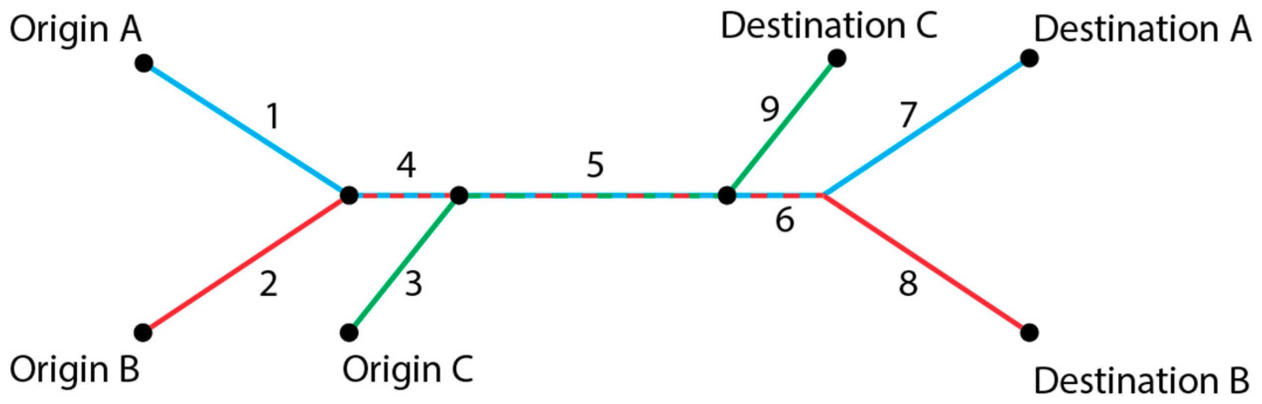
2.1.2. Three-Ship Formation Flight

When a third flight is added to a formation, the number of phases is increased from five to nine. This is schematically depicted in Figure 2.

It is important to note though that, while the number of flight phases is known up front in a three-ship formation assembly (i.e., nine), the sequence of these phases is not known a priori. In Figure 2, it is assumed that Aircraft C is the last aircraft to join the formation, while it is also the first aircraft to leave the formation. However, it is conceivable as well that Aircraft A first joins with Aircraft C, or that Aircraft B first joins with Aircraft C. Similar considerations can be made for the first aircraft leaving the formation, which alternatively could be Aircraft A or B as well. It is clear that Figure 2 displays just one out of nine possible options to assemble/disassemble a three-ship flight formation. Similar to the assembly of a two-ship formation, the assembly of a three-ship formation using the MOC framework always proceeds in compliance with the switching structure that is imposed in a particular option—regardless of whether the assumed structure is valid or not. Clearly, if an inappropriate switching structure is assumed, some of the formation phases might shrink to size zero in the ensuing trajectory optimization process.

In the two-ship formation flight problem considered in Section 2.1.1, combinatorial issues do not play a role. In the two-ship problem, the sequence of flight phases (i.e., the switching structure) is known a priori, resulting in a single multi-phase trajectory optimization solution. In order to accept (or reject) a two-ship multi-phase trajectory optimization solution as the “optimal” solution, it is sufficient to merely compare it to the optimal control solution of the problem in which only solo flights are considered. For the three-ship problem, however, this is not sufficient. In addition to comparing the “best” three-ship solution with solutions where all aircraft remain flying solo, the possibility of two-ship formations in conjunction with a solo flight needs to be considered as well. Clearly, there are three such possible options for a two-ship formation in combination with a single flight. Including the all-solo option, there are therefore 13 possible combinations that can potentially provide the optimal solution to the three-ship problem.

When the number of aircraft that may join in formation is increased even further, the number of sequencing options grows dramatically, clearly illustrating the combinatorial complexity of the multi-ship formation flight trajectory optimization problem. To be able to deal with such problems, a hybrid optimal control (HOC) formulation [19,20,21], which considers both continuous-valued and discrete-valued variables, is called for. The required HOC formulation essentially extends a multi-phase trajectory optimization problem with an integer programming subproblem to reduce the combinatorial complexity associated to the flight phase sequencing problem.

In this study, we have so far not employed a formal hybrid optimal control approach, but rather resorted to exhaustive enumeration to explore all 13 possible flight phase sequencing options in a three-ship formation assembly problem.

2.2. Equations of Motion

The system model adopted in this study to describe the movement of two or three aircraft in a three-dimensional space is the so-called intermediate point-mass model [22]. The intermediate model is a reduced-order point-mass model, based on the assumption of equilibrium of forces normal to the flight path. The resulting equations of motion for a single aircraft (flying either solo or as a formation leader) can be written as:

$$\dot{\varphi }=\frac{V\cos \gamma \sin \chi +V_{W_N}}{R_E+z},$$

(1)

$$\dot{\lambda }=\frac{V\cos \gamma \cos \chi +V_{W_E}}{\left(R_E+z\right)\cos \varphi },$$

(2)

$$\dot{z}=V\sin \gamma ,$$

(3)

$$\dot{V}=\frac{g_0\left(T-D\right)}{W}-g_0\sin \gamma ,$$

(4)

$$\dot{\chi }=\frac{g_0}{V\cos \gamma }\frac{L\sin \mu }{W},$$

(5)

$$\dot{W}=-F_c,$$

(6)

where the state variables are: latitude $\varphi$, longitude $\lambda$, altitude $z$, airspeed $V$, heading angle $\chi$, and aircraft gross weight $W$. The aerodynamic forces considered in the model include the thrust $T$ and the drag $D$. The fuel flow $F_c$ is modelled as a function of speed, altitude, and thrust, i.e., $F_c=F_c\left(V,z,T\right)$. Furthermore, $V_{W_N}$ and $V_{W_E}$ are the wind speed components in, respectively, north-south direction, and east-west direction.

The intermediate point-mass model features three control variables, viz., the engine control setting η, the flight path angle $\gamma$ and the aerodynamic roll angle μ. The engine control setting variable $\eta$, which obeys the constraint $0\le \eta \le 1$, is related to the thrust of the aircraft following:

$$T=\left(T_{max}-T_{min}\right)\eta +T_{min},$$

(7)

where $T_{max}\left(h,V\right)$ and $T_{min}\left(h,V\right)$ are, respectively, the maximum and flight idle thrust of the engine.

The lift force obeys the traditional relation:

$$L=C_{L}qS=C_L\frac{1}{2}\rho V^{2}S,$$

(8)

where $C_L$ is the lift coefficient, $q$ is the dynamic pressure, $S$ is the wing surface area of the aircraft considered, and ρ is the air density.

The drag force is given by:

$$D=C_D\left(C_L\right)qS\Rightarrow D=D\left(z,V,C_L\right),$$

(9)

where $C_D$ is the drag coefficient, which is assumed to obey a parabolic drag polar form:

$$C_D=C_{D_0}\left(M\right)+K\left(M\right)C_L^2.$$

(10)

The expression for the drag coefficient $C_D$ comprises two parts: the induced drag component $K\left(M\right)C_L^2$ and the zero-lift drag component $C_{D_0}\left(M\right)$.

To model the trailing aircraft in a formation flight leg, a simplified system model is made of use. In this model, the altitude and speed dynamics, which drive the leading aircraft, are used to govern the trail aircraft as well, ensuring that the flights that make up a formation string basically operate as a single entity.

It is noted that the drag and weight characteristics of the trailing aircraft in a formation are generally not the same as for the lead aircraft, and therefore the thrust levels needed for station keeping are different from the lead aircraft as well. The thrust level required by the (single or two) trailing aircraft can be readily obtained from the specific energy rate balance:

$${\dot{E}}_{lead}={\dot{E}}_{trail}\Rightarrow {\left[\frac{V\left(T-D\right)}{W}\right]}_{lead}={\left[\frac{V\left(T-D\right)}{W}\right]}_{trail},$$

(11)

and, consequently:

$$\begin{array}{c}{T}_{trail}={\left[\frac{\left(T-D\right)}{W}\right]}_{lead}·W_{trail}+D_{trail},\\ \mathrm{subject} \mathrm{to}: 0\le {\eta }_{trail}=\frac{\left(T_{trail}-T_{min}\right)}{\left(T_{max}-T_{min}\right)}\le 1.\end{array}$$

(12)

Note that specific energy $E$, introduced in Equation (11), is defined as the sum of potential and kinetic energy:

$$E=z+\frac{V^2}{2g_0}.$$

(13)

A traditional parabolic drag polar is assumed for all aircraft. However, for each trail aircraft in a formation, the lift drag polar is extended with a factor $\epsilon$ in order to model the reduction in the induced drag coefficient resulting from formation flight:

$$C_D=C_{D_0}+\left(1-\epsilon \right)K{C}_L^2.$$

(14)

Similar to [18], an induced drag coefficient reduction of 25% ($\epsilon$ = 0.25) is assumed as a baseline for the trailing aircraft within a two-aircraft formation. In a three-ship formation, the second trailing aircraft in the formation typically enjoys a larger induced drag reduction than the first trailing aircraft (flying in the middle) of the string, as it is essentially able to benefit from two wake vortex generators. As pointed out before, the particular formation flight configuration employed (i.e., Echelon formation, V formation or inverted V formation) tends to have a significant influence on the induced drag reduction benefits that can be attained [9]. In this study, the induced drag reduction factor of the first trailing aircraft in a three-ship formation is assumed to remain at 25% (as in a two-ship formation), while for the second trailing aircraft it is assumed to increase to 50%. The latter assumption is consistent with the observation in [9] where it is observed that three-aircraft formations can provide about 13% additional formation induced drag savings (on average) relative to two-ship formations.

2.3. Optimization Criteria

The performance objective considered in this study is to minimize the overall fuel burn of all aircraft in the considered flight formation. The performance criterion that has been implemented in the optimization framework is a composite performance index representing the direct operation cost (DOC). The DOC criterion is essentially a weighted combination of time and fuel costs. DOC-optimized formation flight trajectories have been extensively studied in [18]. In this study, the focus is more environmentally oriented, and the minimum fuel-burn criterion considered herein is assumed to be a good proxy for minimum CO₂ emission. The fuel-optimal solution can be obtained by setting the weighting factor for time cost to zero in the DOC criterion.

The performance index related to the total fuel burn of flights is defined separately for the solo flights and the formation flight missions. For a solo mission, the total fuel burn is determined by aggregating the fuel consumption for all city-pair solo flights considered:

$$J_{fuel,solo}={\displaystyle \sum }_j^{j_{max}}\left[W_j\left(t_{0,j}\right)-W_j\left(t_{f,j}\right)\right],$$

(15)

where the index $j$ relates to the flights A ($j=1$), B ($j=2$) or C ($j=3$) and $j_{max}$ is the total number of flights considered (2 or 3).

In a formation flight mission, the fuel consumption criterion is determined by aggregating the fuel-consumed in the five (two-ship) or nine (three-ship) flight phases:

$$J_{fuel,formation}={\displaystyle \sum }_i^{i_{max}}\left[W_i^C\left(t_{0,i}\right)-W_i^C\left(t_{f,i}\right)\right],$$

(16)

where $W_i^C$ is the combined weight of all aircraft in flight phase $i=1,\dots ,i_{max}$, where $i_{max}=5$ (two-ship formation) or $i_{max}=9$ (three-ship formation).

2.4. Constraints, Staging and Boundary Conditions

In the formation flight multi-phase optimal control formulation, a variety of boundary conditions and path/control constraints have been imposed. The boundary conditions include the values of the position coordinates (longitude, latitude), speed, altitude and heading at both the initial and final time, for all flights considered.

With respect to the timing constraints for the flights, two different cases can be distinguished, the synchronized case and the non-synchronized case. In the synchronised case, neither the initial times nor the final times of the flights are specified. Instead, simply the time at which the first rendezvous takes place is fixed upfront. In the assembly of a two-ship formation there is only a single rendezvous, but in the assembly of a three-ship flight formation there are two instances at which rendezvous takes place (see Figure 2). In a synchronized scenario, the departure times of the participating aircraft are essentially synchronised in the trajectory optimization process to achieve the lowest possible (fuel) cost.

In a non-synchronized scenario, the departure times of the participating flights are fixed as boundary conditions, while no constraints on the rendezvous times are imposed.

In the case study presented in Section 4, only results pertaining to fully synchronized scenarios will be shown. Results for a non-synchronized scenario have been presented in [18]. Notably, it has been shown in [18] that two thirds of the fuel savings obtained through formation flight can be preserved if one of the flights is delayed by half an hour.

Perhaps the most elaborate set of constraints/boundary conditions that have been imposed relate to the specification of the initial and final weights of the flights participating in the formation. In general, an aircraft needs to take enough fuel on board to reach the intended destination—plus a required reserve. This required reserve typically consists of contingency fuel and a final reserve fuel. Similar to [18], the reserve fuel has been assumed to be 5% of the trip fuel in this study.

For aircraft flying a solo mission, or as the leader in a formation, the final gross weight of the aircraft is taken as the sum of the operational empty weight (OEW), the payload ($W_{payload}$) and a fuel reserve of 5% of the overall fuel capacity ($W_{FC}$):

$$W_i\left(t_{f,i}\right)=OEW+W_{payload}+0.05W_{FC}, i=A,B.$$

(17)

With the final weight determined according Equation (17), the unspecified initial weight of the aircraft (solo or formation leader) is subsequently determined in the trajectory optimization process.

However, the assessment is more involved for aircraft trailing in a formation. When flying in formation, trailing aircraft generally enjoy an induced drag reduction and an associated fuel burn saving. However, a designated trailing aircraft might not be able to benefit from such a drag reduction when, due to contingency circumstances, it is not able to join up with the intended formation partner(s). To allow for this contingency, more fuel than needed has to be carried in order to fly in formation (whilst maintaining an adequate fuel reserve). To deal with this issue, additional constraints have been introduced in the multiphase optimal control formulation, which ensures that the initial weight of a trailing aircraft is determined, so that it would be able to fly the (longer) formation route solo in case the designated formation flight partners do not show up (refer to [18] for the details of this constraint mechanism).

Another important set of constraints in a multi-phase formulation relate to the so-called staging conditions that essentially specify how the state at the end of a particular phase is connected to the initial state in the next phase. The staging conditions in this study are rather simple in regards that the initial state of a particular phase is directly and fully linked to the final state of a preceding phase. Figure 1b illustrates how the five phases in the assembly of a two-ship formation are connected through four staging conditions:

• Link 1:   Links phase 1 to phase 3
• Link 2:   Links phase 2 to phase 3
• Link 3:   Links phase 3 to phase 4
• Link 4:   Links phase 3 with phase 5

The eight linking conditions associated to the assembly/disassembly of a three-ship formation (see Figure 2) are very similar in nature:

• Link 1:   Connects phase 1 with phase 4
• Link 2:   Connects phase 2 with phase 4
• Link 3:   Connects phase 3 with phase 5
• Link 4:   Connects phase 4 with phase 5
• Link 5:   Connects phase 5 with phase 6
• Link 6:   Connects phase 5 with phase 9
• Link 7:   Connects phase 6 with phase 7
• Link 8:   Connects phase 6 with phase 8

When assembling a flight formation, it is important to decide beforehand which aircraft is designated as the formation flight leader. In [18], it is shown that for the aerodynamic model considered herein, the best choice is to designate the least heavy aircraft as the leader, as the heavy aircraft can benefit relatively more from an induced drag reduction. The same strategy has been adopted in this study.

3. Trajectory Optimization Framework

Many direct and indirect techniques are available for resolving a multi-phase trajectory optimization problem [23]. As noted in [23], pseudospectral methods are considered some of the most computationally effective families among the global collocation techniques available for the direct resolution of nonlinear trajectory optimization problems. In this study, the so-called Radau pseudospectral method [24] has been selected for resolving the MOC problem. More specifically, the multi-phase optimal control framework that has been developed, implements the MATLAB-based general-purpose pseudospectral optimal control tool GPOPS (general pseudospectral optimal control software) [25]. The pseudospectral method essentially transcribes the multi-phase trajectory optimization problem into a non-linear programming (NLP) problem. The resulting large-scale NLP problem is solved using the SNOPT (sparse nonlinear optimizer) tool which is used in conjunction with IntLab (interval laboratory), a third-party automatic differentiation tool within the GPOPS-based framework.

4. Case Study

To investigate the benefits and characteristics of two-ship and three-ship formation flights, a case study has been set up, comprising a large number of numerical experiments. In all experiments of the case study, the trajectories are optimized for minimum fuel, and Aircraft B is always assumed to be the lead aircraft of the formation. Moreover, standard atmospheric conditions have been assumed (either with or without the presence of a wind field) in all numerical experiments.

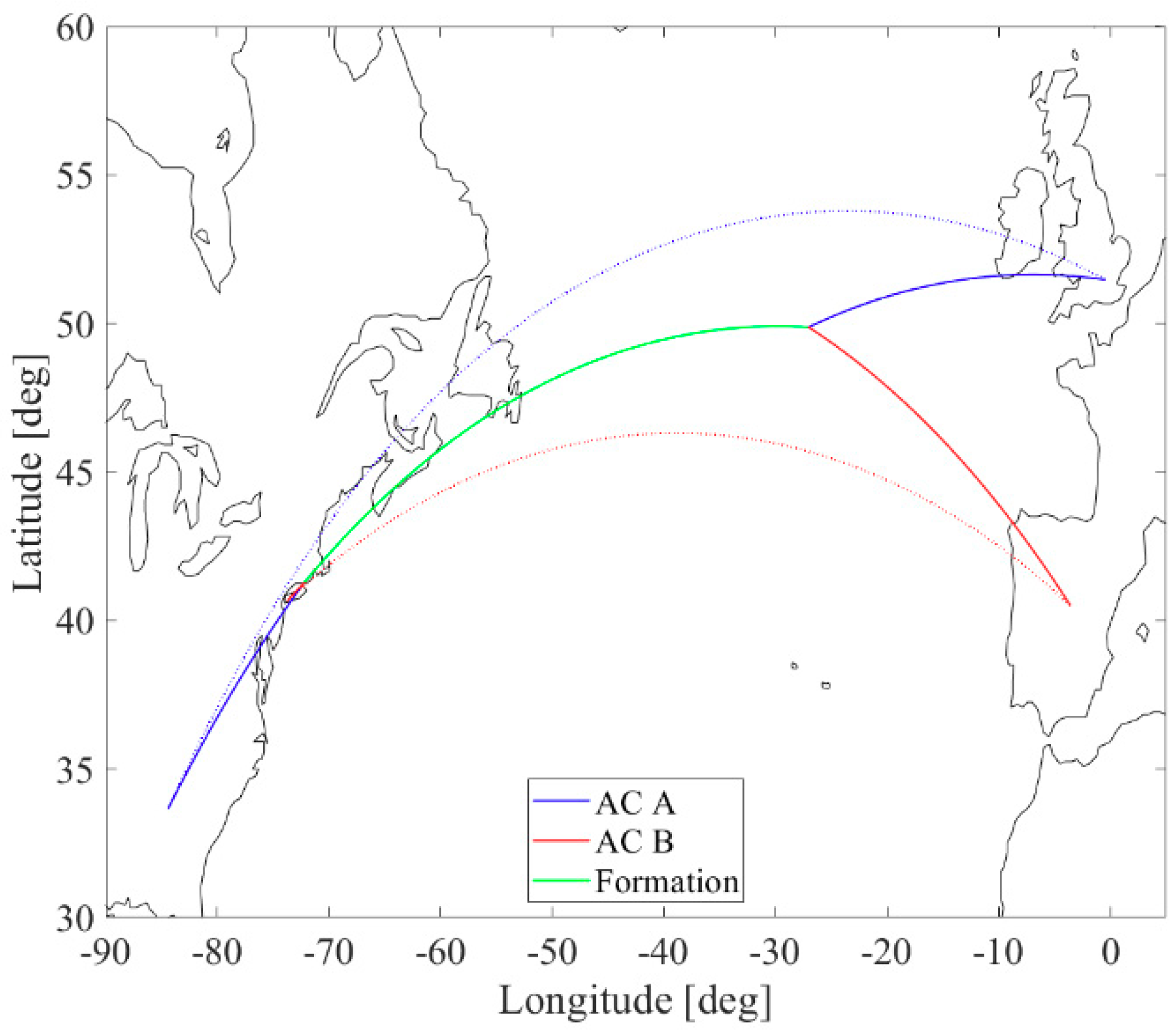
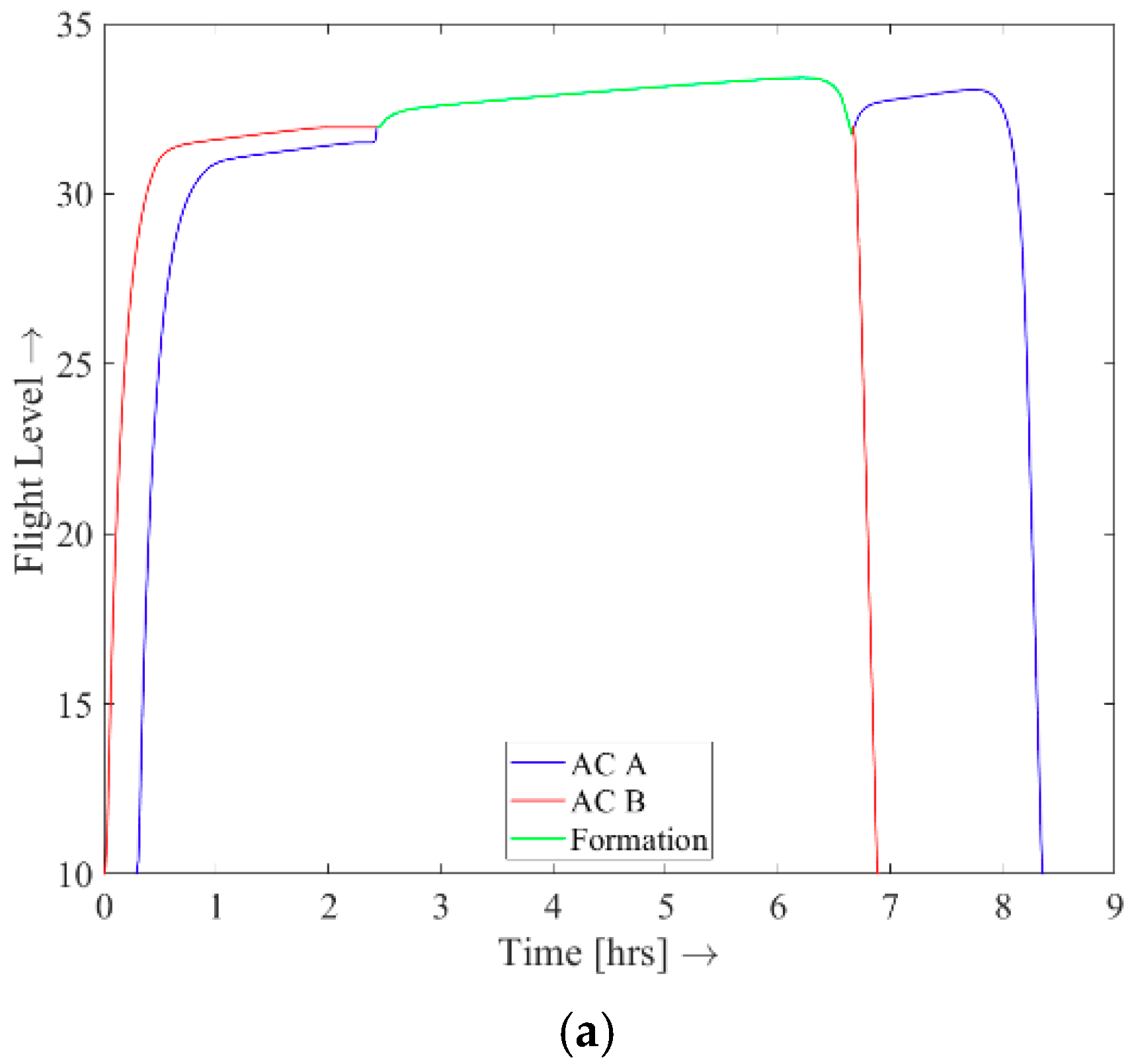
4.1. Baseline Scenario

The baseline scenario considered is the same as the scenario considered in the study presented in [18]. In this baseline scenario, a no-wind assumption has been made and the following two flights are assumed to join in formation:

• Aircraft A: B744 (i.e., B747-400) from London (LHR) to Atlanta (ATL)
• Aircraft B: B744 from Madrid (MAD) to New York City (JFK)

It is noted that Aircraft B (being the least heavy of the two) is assigned as the lead aircraft in a formation. The two flights considered in the baseline scenario are assumed to be perfectly synchronized with respect to their departure times. The results for the baseline scenario have been generated using the same aircraft performance model (Boeing B747-400, wide-body aircraft) that was considered in the study presented in [26].

The optimal ground tracks found for the baseline scenario are presented in Figure 3, while the corresponding vertical flight paths and velocity profiles are presented in Figure 4a,b, respectively.

When examining the trajectory solution in the vertical plane, perhaps the most striking features that can be observed are the rapid transitions in the speed and altitude histories close to the joining point. As discussed in [18], the slightly higher cruise altitude and slightly lower cruise speed in formation flight (relative to flying solo) are a direct consequence of the fact that a better drag to speed ratio can be attained at these conditions when flying in formation. The study presented in [27] supports this finding.

Another striking feature previously observed in [18], is that the two-ship formation in fact starts descending before it breaks up. After the break-up of the formation, Aircraft A begins to climb again to attain the most favorable cruise conditions for solo flight.

Table 1. Results for the baseline scenario.

Results	Solo Flight			Formation Flight
	Aircraft A	Aircraft B	Total	Aircraft A	Aircraft B	Total
Fuel (kg)	79,093	66,239	145,332	75,530	67,238	142,768
Time (h)	7.92	6.80	14.71	8.09	6.90	14.99
Distance (km)	6768	5760	12,529	6825	5835	12,660

summarizes the most important results for the baseline case. Although the fuel burn of the leading Aircraft B increases in comparison to flying solo, the total fuel-consumed in the formation flight mission decreases with about 1.8%.

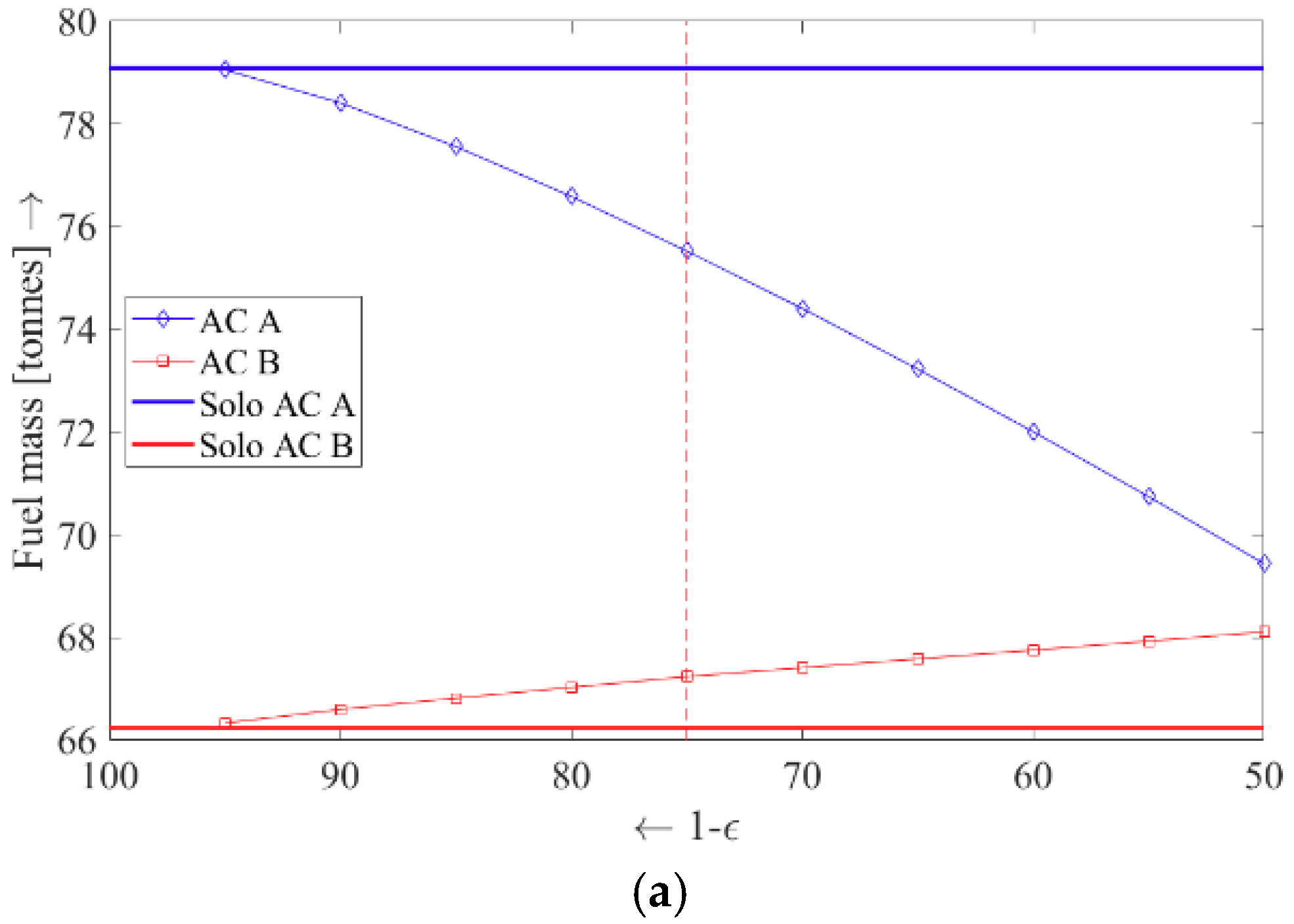
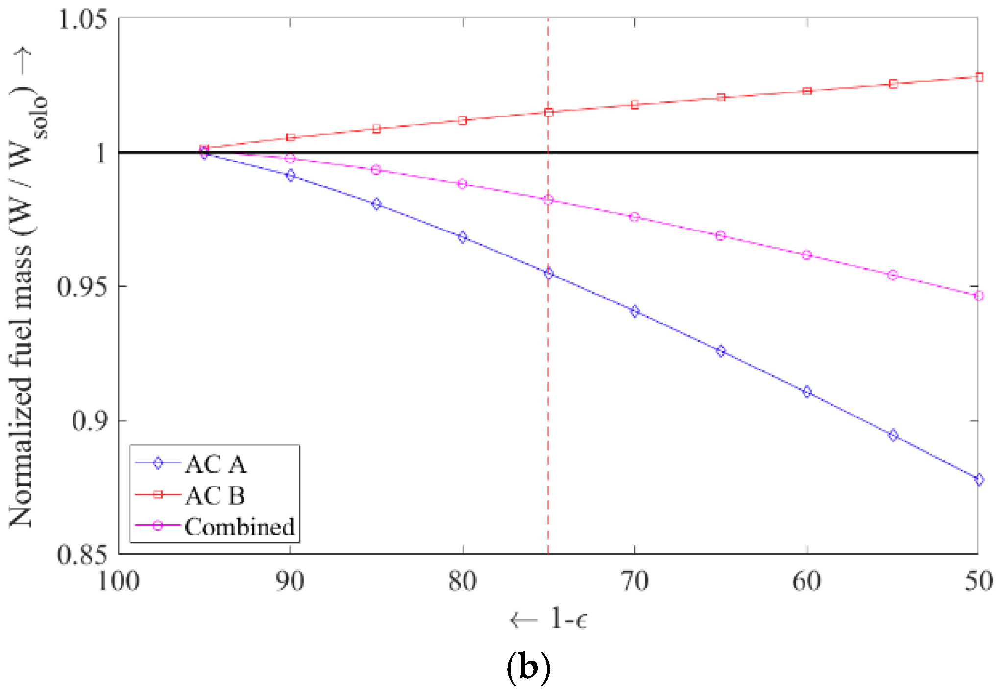
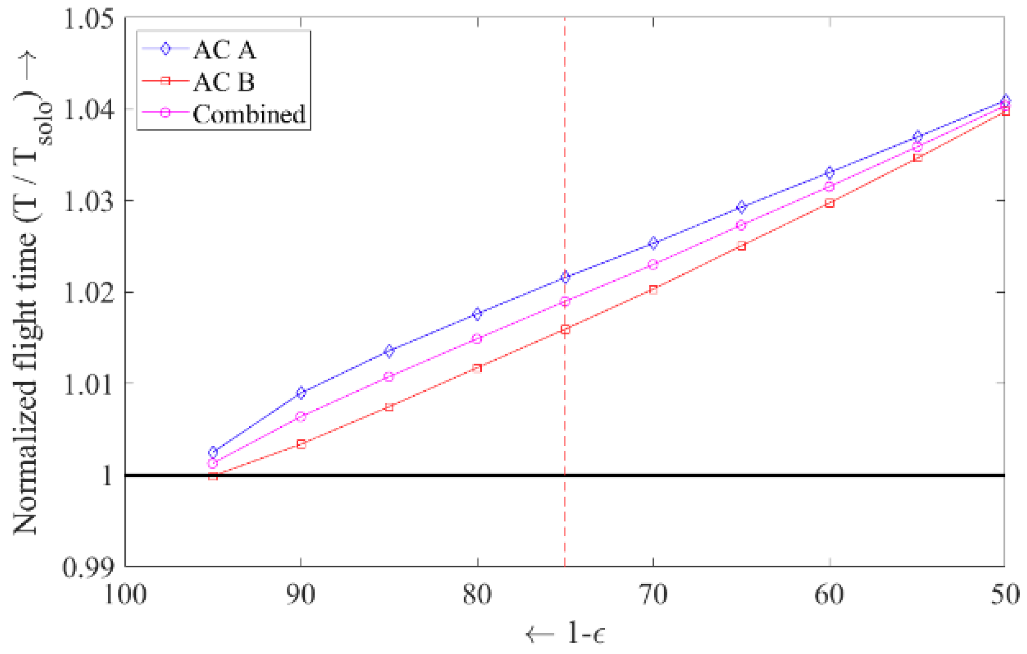
4.2. Sensitivity Analysis

In the baseline scenario, a default induced drag reduction factor of 25% has been assumed, based on the study presented in [4]. However, the various research studies that have been conducted to quantify the potential aerodynamic benefits of (extended) formation flight show a relatively large spread of the performance benefits, featuring reductions in induced drag of the trailing aircraft anywhere between 10% and 70% [28]. Moreover, as pointed out in the introduction, the aerodynamic performance of trailing aircraft in a flight formation is highly dependent on a number of factors, including the aircraft types/sizes in the formation, the formation flight configuration, and the station keeping performance.

In view of the uncertainty in establishing the actual induced drag reduction that can be attained in formation flight, a sensitivity analysis has been conducted in which the induced drag reduction factor $\epsilon$ is varied from 0% to 50%. Excepting the induced drag parameter value, the scenario that is considered in the sensitivity study is the same as in the two-ship baseline.

In Figure 5, the ground tracks of the optimal formation flight solutions are shown for various values of the induced drag reduction factor (green lines), along with the original optimal solo flights (white lines). It can be observed in Figure 5 that the rendezvous point location for this set of flights changes significantly with the assumed value of the induced drag reduction parameter. For the case featuring the largest reduction in induced drag (50%), the easternmost rendezvous point location is obtained; this location shifts to a western direction when the induced drag reduction factor is decreased. Note that the rendezvous point pertaining to the baseline solution presented in Section 4.1 is labeled in orange.

The resulting fuel consumptions and flight times are plotted in Figure 6 and Figure 7. In Figure 6a, fuel consumption is plotted as a function of the induced drag reduction factor $\epsilon$ for each aircraft separately, whilst in Figure 6b the fuel burn—normalized with respect to the solo flights—is shown. From the fuel burn curves in Figure 6a it can be observed that the fuel burn of the lead aircraft (Aircraft B) increases almost proportionally with the induced drag reduction factor caused by the route detour, whilst the fuel consumption of the trailing aircraft decays with increasing value of induced drag reduction factor to a far stronger degree. The gradually stronger decrease in fuel consumption of the trailing aircraft can be attributed to the fact that the common formation segment increases in size when the value of the induced drag reduction parameter increases. A close inspection of the results shown in Figure 6b, shows that fuel savings can be attained by flying in formation for any value of induced drag reduction factor in excess of 5% ($\epsilon$ > 0.05). Note that the red dotted vertical line shown in Figure 6a,b represents the solution of the baseline case ($\epsilon$ = 0.25).

In Figure 7, the optimal flight times are plotted against the induced drag reduction factor. In the figure, the flight time normalized with respect to the solo flights is presented. Not surprisingly, the travel time for all aircraft joining in formation is larger relative to the solo flights. Clearly, the trip times increase even further when the formation flight induced drag reduction factor increases. This is caused by the fact that a larger detour to rendezvous is generally required when the extent of the formation flight leg increases.

In Figure 7, the baseline results are again highlighted by vertical red dotted lines. It can be noted that a small decrease or increase of the induced drag reduction parameter value relative to the baseline value (e.g., by 5%) leads to only slightly different results in terms of flight times and fuel consumption. Although this sensitivity analysis has been performed for a particular set of flights, the conclusions are likely to be similar for any pair of Origin/Destination flights that prove eligible to join in formation.

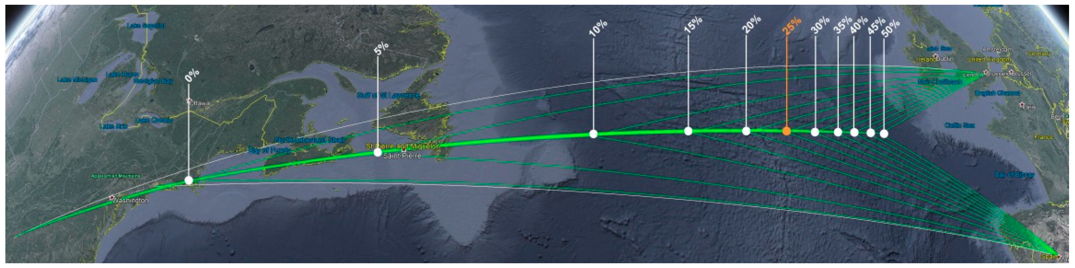
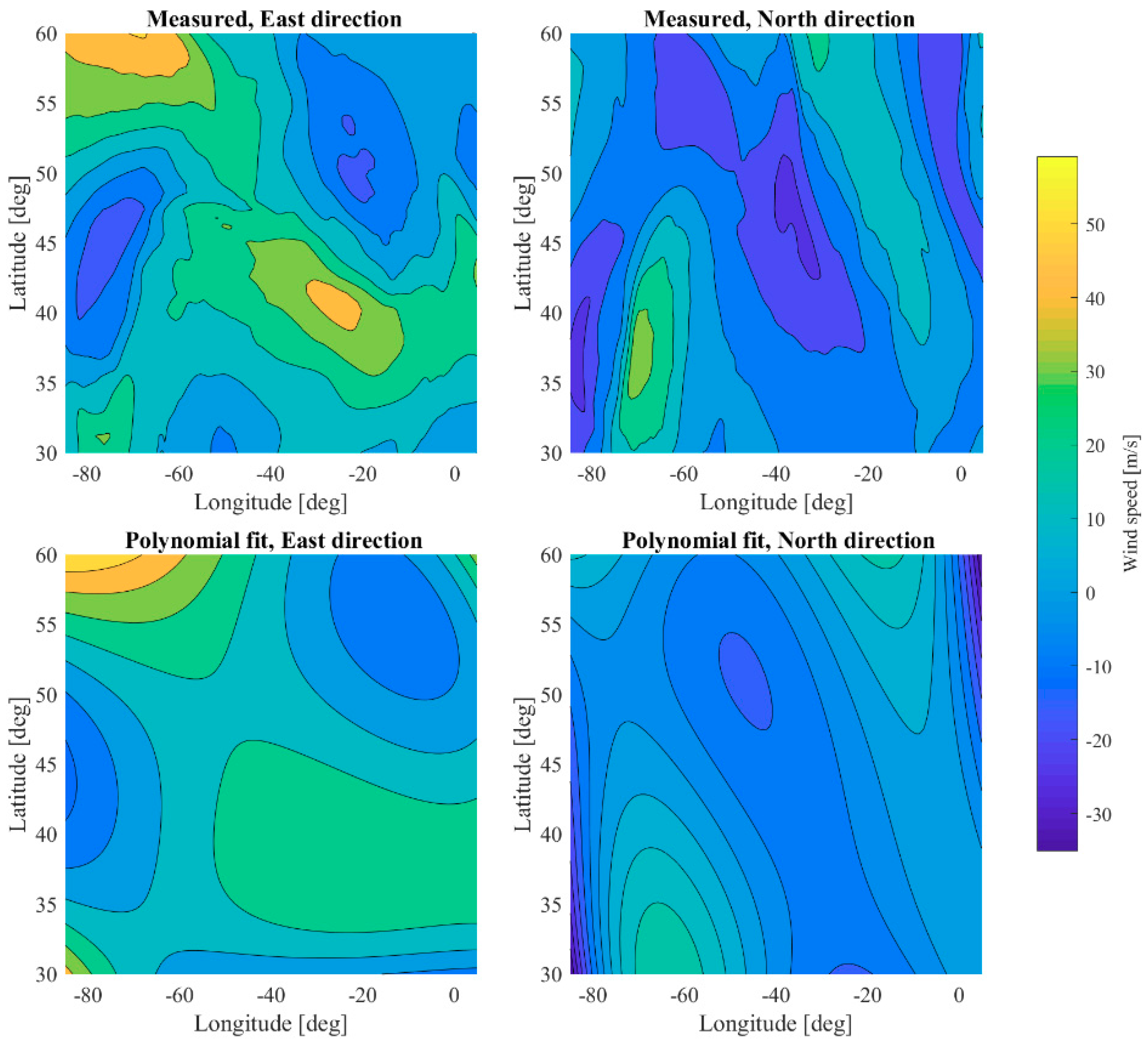
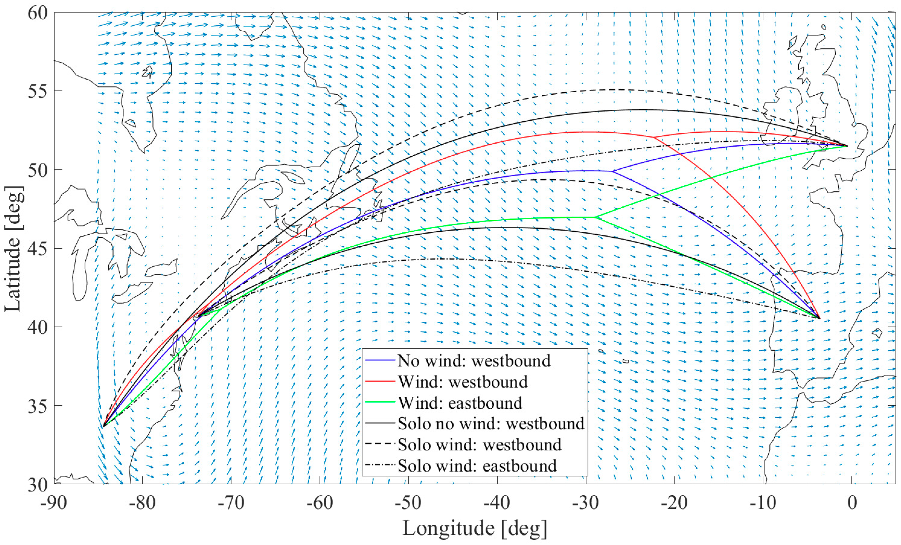
4.3. Formation Flight in the Presence of Wind

In real-world operations, aircraft almost never follow the shortest possible path from their origin to their destination—even though this path represents the optimal route from a geometric perspective. The reason is that aircraft always need to take the ambient weather conditions into account—especially the wind conditions. In the presence of wind, aircraft may deviate from the shortest path in order to avoid encountering strong headwinds or to profit from areas with favourable tailwinds.

To handle the demand in air traffic in the busiest part of the North Atlantic region—where there is essentially no radar coverage—the so-called North Atlantic organised track system (NAT-OTS) is used to ensure that aircraft remain safely separated. NAT-OTS concerns a structured set of transatlantic flight routes that connect North America to Western Europe in order to accommodate the traffic waves—typically consisting out of four to eight parallel tracks in eastbound direction and four to eight parallel tracks in westbound direction. The NAT-OTS routes, which are published on a daily basis, are optimized to provide the minimum time routes (MTRs) for aircraft, taking the prevailing wind conditions into account. The study presented herein does not consider an organized track system, however; the effect of wind on the synthesis of minimum-fuel formation flight trajectories is studied based on similar weather information as employed in the generation of NAT-OTS tracks.

The Meteorological Service of Canada has made a GRIB2 format database publicly available. It contains data from analysis systems along with output from Canadian Meteorological Centre’s Numerical Weather Prediction (NWP) models [29]. The so-called Global Deterministic Forecast System (GDPS) data is defined on a latitude–longitude grid featuring a 0.6° resolution (≈66 km) and is vertically covered by 28 isobaric levels distributed over an altitude range from approximately 100 to 19,300 m.

To support the trajectory optimization framework that we have developed, a functionality that provides a multitude of local atmospheric properties for any given set of position coordinates and pressure altitude has been conceived. This functionality retrieves the atmospheric properties (notably wind speed components and temperature profiles) at a given location by interpolating the GDPS data over the defined grid for a selected date and time. However, an International Standard Atmosphere can optionally be selected as well. Since the employed NLP solver requires a smooth interpolated surface (differentiability requirement), cubic interpolation for 3D gridded data has been used. The spline approximation employed here is similar the approximation adopted in [30]—albeit in [30] the spline approximation is made in two dimensions, assuming flight at a constant pressure altitude. The major downside of the tricubic interpolation approach adopted in this study is that it results in a significant computational burden for calculating optimal formation flight trajectories.

To demonstrate the impact of wind on the assembly of formation flights, a simple numerical example that does not make direct use of the implemented weather database will be presented. Rather, the example is based on a simple analytic model of a wind field that has been synthesized from the weather database in a confined region at a particular date and time. In the analytic model, the wind does not vary with altitude; in each grid cell, the average wind observed in the altitude, which ranged between 5000 to 15,000 m, has been used in this study. Since the main purpose of this example is to demonstrate the effect of the wind on formation routing (notably, on the location of joining and splitting points), obtaining a perfect representation of the actual wind-field at a given date and time was not considered to be crucial in this case study.

To obtain smooth functions for describing the wind components over the North-Atlantic area, the wind data points at the defined grid have been fitted by polynomial regression in this numerical example. The approach taken is similar to that employed in [30]. More specifically, a polynomial surface of degree 4 in both latitude $\varphi$ and longitude $\lambda$ has been fitted for the wind components in a north-south direction ($V_{W_N}$) and in an east-west direction ($V_{W_E}$), respectively. In Figure 8, the wind-field components $V_{W_N}$ and $V_{W_E}$ in the North Atlantic region, measured on 24 May 2016, are plotted (top), as well as the polynomial fit used in this case study (bottom). Although the overall goodness of the surface fit is not great (R² = 0.63 for $V_{W_E}$; R² = 0.43 for $V_{W_N}$), the most essential features of the wind field are still captured. The main advantage of using the polynomial surface fit relative to directly interpolating the wind data over the defined grid is that the computational burden of calculating optimal formation flight trajectories is reduced significantly.

In the baseline scenario the considered flights are from Europe towards North-America (westbound). To compare the wind impacts, two sets of flights were compared in the wind field scenario considered here: a set of westbound flights (the same as considered in the baseline scenario) and a set of eastbound flights (the same flights but with origin and destination airports swapped). Aircraft A is the trailing aircraft in both instances.

The resulting optimal ground tracks for the wind field scenario are presented in Figure 9. The ground track corresponding to the baseline solution (Section 4.1) has been included in the figure as well. It can be observed that the wind over the North-Atlantic Ocean is mainly blowing in an eastern direction. When considering the (solo and formation flight) ground tracks shown in Figure 9, it can be noted that the westbound flights in wind conditions (red) fly further north than the optimal flight paths in the no-wind condition (blue), whilst the eastbound flights (green lines) fly further south. Indeed, the eastbound flights deviate in a southern direction in order to benefit from the stronger tailwinds in that region, while the westbound flights deviate to the north in order to minimize the headwinds which they encounter. Additionally, the significant difference in duration of the formation segments in eastbound and westbound directions is worth noting; the eastbound flights fly in formation during 3.8 h and for the westbound flights during 4.7 h.

The performance results for the westbound and eastbound flights are summarized in

Table 2. Results for the wind field scenario, westbound.

Results	Solo Flight			Formation Flight
	Aircraft A	Aircraft B	Total	Aircraft A	Aircraft B	Total
Fuel [kg]	80,549	70,798	151,347	76,307	71,708	148,015
Time [h]	7.98	7.04	15.03	8.12	7.19	15.32
Distance [km]	6786	5823	12,609	6792	5986	12,780

and

Table 3. Results for the wind field scenario, eastbound.

Results	Solo Flight			Formation Flight
	Aircraft A	Aircraft B	Total	Aircraft A	Aircraft B	Total
Fuel [kg]	77,285	61,130	138,415	74,296	61,989	136,285
Time [h]	7.84	6.53	14.37	8.02	6.62	14.64
Distance [km]	6810	5799	12,609	6960	5785	12,746

, respectively. The results for the corresponding flight in the absence of wind are summarized in Table 1. Inspection of the results shows that the eastbound flights burn less fuel than the westbound flights due to the prevailing winds (primarily in the eastern direction). Relative to the no-wind baseline solution (Table 1), slightly more than 4% savings in fuel burn can be obtained for eastbound flights, while the increase in fuel burn is slightly less than 4% for westbound flights. Flying the formation routes in a westbound direction results in an increase in total flying time for the formation of about 4% as well. In contrast, flying the formation in the eastbound direction hardly saves time relative to the no-wind baseline solution.

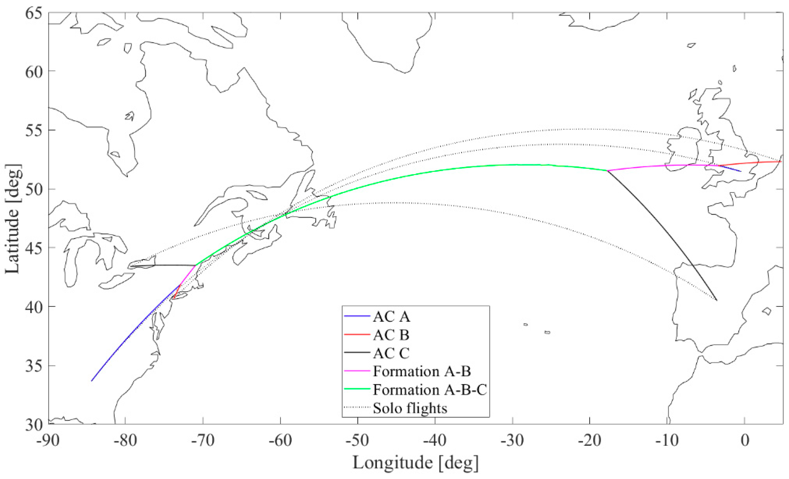
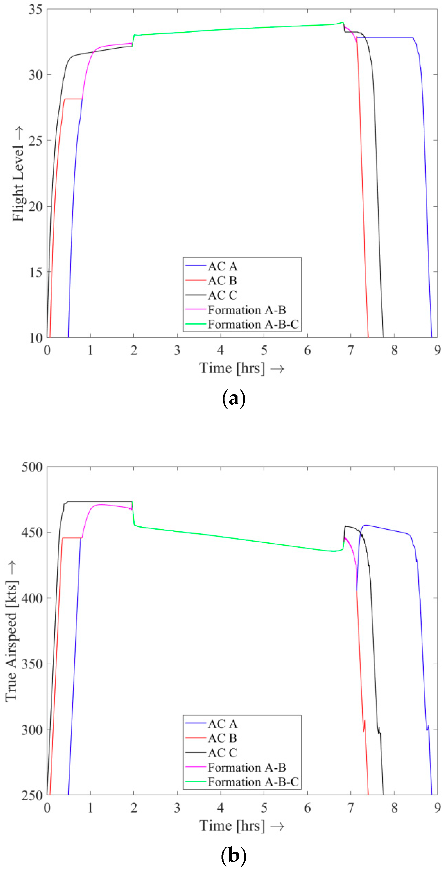
4.4. Three-ship Formation Flight

In the previous section, we demonstrated that two-aircraft formations can already result in significant fuel burn reduction relative to flying solo. When more aircraft join a formation, this is likely to result in even higher savings, as more aircraft will benefit from a reduction in induced drag. A two-ship formation features one leading aircraft and one trailing aircraft. However, when more aircraft join a formation, the number of trailing aircraft (which enjoy an induced drag reduction) increases, while the number of leading aircraft remains one. Next to this, as described in Section 2.2, the overall induced drag reduction that can be attained increases as well when the formation becomes larger. The aim of the present numerical example is to demonstrate that the developed multi-phase trajectory optimization tool is able to synthesize three-ship formations, as well as to explore the fuel burn benefits that larger formations might have.

In this numerical example, three flights (B744) from Europe to North-America seek to join in formation:

• Aircraft A: B744 from London to Atlanta
• Aircraft B: B744 from Amsterdam to New York City
• Aircraft C: B744 from Madrid to Toronto

Similar to the two-ship formation assembly examples presented in the previous sections, a scenario is here considered where all flights seeking to join the formation are perfectly synchronized in terms of departure times. A no-wind condition is assumed in this three-ship formation flight example.

As outlined in Section 2.1.2 for the three-ship formation assembly problem, there are 13 possible options with respect to the assumed phase switching structure. Here, only two of these 13 options will be presented, viz., the best-performing (three-ship formation) option, and the all-solo option. The latter option is included to provide a basis of comparison.

The phase switching structure associated to the best-performing solution corresponds to the structure shown earlier in Figure 2. In this structure, Aircraft A first joins with Aircraft B and subsequently Aircraft C will join the formation.

In Figure 10, the ground tracks of the best-performing three-ship formation solution are shown. Note that Aircraft A is the trailing aircraft during the two-aircraft formation phases, Aircraft B is the leading aircraft during all formation phases and Aircraft C is the trailing aircraft in the three-aircraft formation phase. In other words, during the formation phases, Aircraft A enjoys a 25% reduction, Aircraft B has no reduction and Aircraft C attains a 50% reduction in induced drag. The optimal joining sequence obtained in this example turns out to be convenient from an operational perspective as well, as there is no need to break up the formation in order to permit Aircraft C to join or leave the formation.

The results for this numerical example are summarized in

Table 4. Results for the three-ship formation example.

Results	Solo Flight				Formation Flight
	AC A	AC B	AC C	Total	AC A	AC B	AC C	Total
Fuel [kg]	79,093	67,338	69,934	216,365	71,229	69,065	60,907	201,201
Time [h]	7.92	6.89	7.12	21.94	8.25	7.25	7.67	23.17
Distance [km]	6768	5854	6059	18,681	6806	5956	6340	19,104

. Table 4 compares the performances with respect to fuel burn and flight time of the three (optimal) solo flights A, B and C, with the optimal three-ship formation. The overall reduction in fuel burn achieved in the optimal three-ship formation solution is considerable, amounting to about 7% (relative to flying solo).

In Figure 11, the altitude and velocity profiles corresponding to the three-ship formation flight solution are shown. What is particularly striking in the profiles shown, is that the cruise altitude in the three-ship formation flight leg is increased further relative to the baseline two-ship solution (see Figure 4), whilst cruising the three-ship formation slows down even more significantly than the two-ship formation. As explained in [18], the reduction in optimal cruise speed can be directly attributed to the reduction of the overall induced drag due to formation flight. Similar to the baseline two-ship solution, it can be observed that when Aircraft A and C leave the formation, airspeed is initially increased before descending.

5. Conclusions

This study has described the development of a numerical tool for calculating minimum-fuel formation flight trajectories of long-haul commercial aircraft. Using the developed multi-phase trajectory optimization tool, the benefits and characteristics of two-ship and three-ship formation flights in real-world (weather/wind) conditions have been explored.

To account for the uncertainty in the actual induced drag reduction benefits that can be attained in formation flight, a sensitivity analysis has been conducted to assess how the fuel performance is affected by the degree of induced drag reduction that is enjoyed by aircraft trailing in a formation. The results indicate that the length of the formation flight legs in the optimal trajectory solutions increases with the assumed size of the induced drag reduction parameter. The overall reduction in fuel burn is nearly proportional to the magnitude of the induced drag reduction attained by the trailing aircraft. However, the overall flight time nearly proportionally increased as well with the value of the induced drag parameter.

Experiments have been carried out to assess the influence of the presence of a wind field on formation flight performance and trajectory shaping. It has been shown that the presence of a wind field has significant influence on the location of the optimal ground tracks across the ocean. In the presence of wind, aircraft will generally deviate from their geometrically optimal path so as to avoid areas with large headwinds or to search for areas with favourable tailwinds. Flying with tailwind conditions can reduce the flight time and fuel consumption in formation flight significantly. The experiments related to assessing the impact of wind have been carried out using rather simplified wind field models. For flight planning purposes, more accurate wind field approximations would be required, however, as pointed out in [30], there is clear trade-off between accurate wind modelling and solvability. In future research, the effects of meteorological uncertainty on formation flight planning will need to be explored in detail. In particular, a sensitivity study will be set up to explore how sensitive the locations of the joining and splitting points are to errors in the wind field modelling.

In this study it has been shown that the optimal assembly of three-ship formations is significantly more involved than the assembly of two-ship formations. While the two-ship formation problem can be readily formulated and solved as a relatively simple multi-phase optimal control problem (with an a priori known switching structure), the three-ship formation problem manifests itself as a more complicated hybrid optimal control problem (with an unknown switching structure). The hybrid optimal control formulation essentially combines the multi-phase trajectory optimization problem with an integer programming subproblem for resolving the flight phase sequencing problem. In this study, we have so far not employed a formal hybrid optimal control approach, but rather resorted to exhaustive enumeration to explore all possible flight phase sequencing options in a three-ship formation assembly problem. The results indicate that larger formations can be significantly more beneficial in terms of fuel savings in comparison to two-ship formation flights.

Future research will focus on the development of a hybrid optimal control framework, permitting the assembly of flight formations of arbitrary size. Additionally, research will be focused on exploring the regulatory and operational aspects associated to the introduction of formation flights, such as air traffic management. Airline alliance economic aspects, such as the sharing of the schedule “shift” (and economic benefits) between flights in order to accommodate the formation, need to be investigated as well.

References

1. Pahle, J.; Berger, D.; Venti, M.; Duggan, C.; Faber, J.; Cardinal, K. An Initial Flight Investigation of Formation Flight for Drag Reduction on the C-17 Aircraft. In Proceedings of the AIAA Atmospheric Flight Mechanics Conference, Minneapolis, MN, USA, 13–16 August 2012; p. 13. [Google Scholar]
2. Nangia, R.K.; Palmer, M.E. Formation Flying of Commercial Aircraft, Variations in Relative Size/Spacing—Induced Effects and Control. In Proceedings of the AIAA Applied Aerodynamics Conference, Miaml, FL, USA, 25–28 June 2007. [Google Scholar]
3. Bower, G.C.; Flanzer, T.C.; Kroo, I.M. Formation Geometries and Route Optimization for Commercial Formation Flight. In Proceedings of the AIAA Applied Aerodynamics Conference, San Antonio, TX, USA, 22–25 June 2009; p. 18. [Google Scholar]
4. Xue, M.; Hornby, G.S. An Analysis of the Potential Savings from Using Formation Flight in the NAS. In Proceedings of the AIAA Guidance, Navigation, and Control Conference, Minneapolis, MN, USA, 13–16 August 2012; p. 12. [Google Scholar]
5. Marks, T.; Linke, F.; Gollnick, V. Evaluation of potential fuel savings by introducing formation flight on a North Atlantic scenario. In Proceedings of the 5th International Air Transport and Operations Symposium (ATOS), Delft, The Netherlands, 20–23 July 2015. [Google Scholar]
6. Liu, Y.; Stumpf, E. Estimation of Vehicle-Level Fuel Burn Benefits of Aircraft Formation Flight. J. Aircr. 2017, 55, 853–861. [Google Scholar] [CrossRef]
7. Blake, W.; Multhopp, D. Design, Performance and Modeling Considerations for Close Formation Flight. In Proceedings of the 23rd AIAA Guidance, Navigation and Control Conference, Boston, MA, USA, 10–12 August 1998. [Google Scholar]
8. Bramesfeld, G.; Maughmer, M. The Effects on Formation-Flight Aerodynamics Due to Wake Rollup. J. Aircr. 2008, 45, 1167–1173. [Google Scholar] [CrossRef]
9. Ning, S.A.; Flanzer, T.C.; Kroo, I.M. Aerodynamic Performance of Extended Formation Flight. J. Aircr. 2011, 48, 855–865. [Google Scholar] [CrossRef]
10. Veldhuis, L.; Voskuijl, M.; Fransen, B. Formation Flight-Fine-tuning of Theoretical Performance Prediction. In Proceedings of the AIAA Aerospace Sciences Meeting, Grapevine, TX, USA, 7–10 January 2013; p. 17. [Google Scholar]
11. Kless, J.E.; Aftosmis, M.J.; Ning, S.A.; Nemec, M. Inviscid Analysis of Extended-Formation Flight. AIAA J. 2013, 51, 1703–1715. [Google Scholar] [CrossRef] [Green Version]
12. Ning, S.A.; Kroo, I.; Aftosmis, M.J.; Nemec, M.; Kless, J.E. Extended Formation Flight at Transonic Speeds. J. Aircr. 2014, 51, 1501–1510. [Google Scholar] [CrossRef]
13. Slotnick, J.P. Computational Aerodynamic Analysis for the Formation Flight for Aerodynamic Benefit Program. In Proceedings of the 52nd Aerospace Sciences Meeting, National Harbor, MD, USA, 13–17 January 2014. [Google Scholar] [CrossRef]
14. Xu, J.; Ning, S.A.; Bower, G.; Kroo, I. Aircraft Route Optimiza-tion for Formation Flight. J. Aircr. 2014, 51, 490–501. [Google Scholar] [CrossRef]
15. Kent, T.; Richards, A. Analytic Approach to Optimal Routing for Commercial Formation Flight. J. Guid. Control Dyn. 2015, 38, 1872–1884. [Google Scholar] [CrossRef]
16. Verhagen, C.M.A.; Visser, H.G.; Santos, B.F. A Decentralized Approach to Formation Flight Routing of Long-Haul Commercial Flights. Proc. Instit. Mechan. Eng. Part G J. Aerosp. Eng. 2019, 233, 2992–3004. [Google Scholar] [CrossRef]
17. Doole, M.; Visser, H.G. A Multi-stage Centralized Approach to Formation Flight Routing and Assignment of Long-haul Airline Operations. In Proceedings of the 4th International Conference on Vehicle Technology and Intelligent Transport Systems (VEHITS), Madeira, Spain, 16–18 March 2018. [Google Scholar]
18. Hartjes, S.; Van Hellenberg Hubar, M.E.G.; Visser, H.G. Multiple-phase Trajectory Optimization for Formation Flight in Civil Aviation. CEAS Aeronaut J. 2019, 10, 453–462. [Google Scholar] [CrossRef]
19. Franco, A.; Rivas, D. Optimization of Multiphase Aircraft Trajectories Using Hybrid Optimal Control. J. Guid. Control Dyn. 2015, 38, 452–467. [Google Scholar] [CrossRef]
20. Kamgarpour, M.; Soler, M.; Tomlin, C.J.; Olivares, A.; Lygeros, J. Hybrid Optimal Control for Aircraft Trajectory Design with a Variable Sequence of Modes. In Proceedings of the 18th IFAC World Congress, Milano, Italy, 28 August–2 September 2011. [Google Scholar]
21. Bonami, P.; Olivares, A.; Soler, M.; Staffetti, E. Multiphase Mixed-Integer Optimal Control Approach to Aircraft Trajectory Optimization. J. Guid. Control Dyn. 2013, 36, 1267–1277. [Google Scholar] [CrossRef] [Green Version]
22. Visser, H.G. Airplane Performance Optimization, article eae393. In Encyclopedia of Aerospace Engineering; John Wiley and Sons, Inc.: New York, NY, USA, 2010. [Google Scholar]
23. Gardi, A.; Sabatini, R.; Ramasamy, S. Multi-objective optimisation of aircraft flight trajectories in the ATM and avionics context. Prog. Aerosp. Sci. 2016, 83, 1–36. [Google Scholar] [CrossRef]
24. Francolin, C.; Rao, A.V. Direct Trajectory Optimization and Costate Estimation of State Inequality Path-Constrained Optimal Control Problems Using a Radau Pseudospectral Method. In Proceedings of the AIAA Guidance, Navigation, and Control Conference, Minneapolis, MN, USA, 13–16 August 2012; p. 11. [Google Scholar]
25. Rao, A.V.; Benson, D.A.; Darby, C.L.; Patterson, M.; Francolin, C.; Sanders, I.; Huntington, G.T. Algorithm 902: GPOPS, A MATLAB Software for Solving Multiple-Phase Optimal Control Problems Using the Gauss Pseudospectral Method. ACM Trans. Mathem. Softw. 2010, 37, 1–39. [Google Scholar] [CrossRef]
26. Teengs, M. Model of the Boeing 747-400 with CF6-80C2B1F Engines; Unpublished Report; TU Delft: Delft, The Netherlands, 2006. [Google Scholar]
27. Voskuijl, M. Cruise Range in Formation Flight. J. Aircr. 2017, 54, 2184–2191. [Google Scholar] [CrossRef] [Green Version]
28. Van Hellenberg Hubar, M.E.G. Multiple-Phase Trajectory Optimization for Formation Flight in Civil Aviation. Master’s Thesis, Delft University of Technology, Delft, The Netherlands, 2017. [Google Scholar]
29. Government of Canada. GDPS Data in GRIB2 Format: 66 km. Available online: https://weather.gc.ca/grib/grib2_glb_66km_e.html (accessed on 25 May 2016).
30. García-Heras, J.; Soler, M.; González-Arribas, D. Characterization and Enhancement of Flight Planning Predictability under Wind Uncertainty. Int. J. Aerosp. Eng. 2019, 2019, 6141452. [Google Scholar] [CrossRef]
Figure 1. A schematic representation of the five-phase assembly of a two-ship formation in a horizontal plane (a) and vertical plane (b).
Aerospace 06 00100 g001
Figure 2. A schematic representation of the nine-phase assembly of a three-ship formation.
Aerospace 06 00100 g002
Figure 3. Fuel-optimal formation ground tracks for the baseline scenario [This figure was reprinted by permission from “Springer Nature: CEAS Aeronaut J., 10(2), Multiple-phase Trajectory Optimization for Formation Flight in Civil Aviation, Hartjes, S., Van Hellenberg Hubar, M.E.G., and Visser, H.G., pp. 453–462, Copyright, 2019”].
Aerospace 06 00100 g003
Figure 4. Formation trajectory results for the baseline scenario, featuring the altitude history (a) and airspeed history (b). [This figure was reprinted by permission from “Springer Nature: CEAS Aeronaut J., 10(2), Multiple-phase Trajectory Optimization for Formation Flight in Civil Aviation, Hartjes, S., Van Hellenberg Hubar, M.E.G., and Visser, H.G., pp. 453–462, Copyright, 2019”].
Aerospace 06 00100 g004aAerospace 06 00100 g004b
Figure 5. Rendezvous point locations for a two-ship formation for different values of the induced drag reduction factor.
Aerospace 06 00100 g005
Figure 6. Sensitivity analysis: fuel consumption as a function of the induced drag reduction factor (a) and fuel burn relative to the fuel consumed by the solo flights (b).
Aerospace 06 00100 g006aAerospace 06 00100 g006b
Figure 7. Sensitivity analysis: flight time.
Aerospace 06 00100 g007
Figure 8. Measured and interpolated wind components in the North-Atlantic region on 24 May 2016.
Aerospace 06 00100 g008
Figure 9. Fuel-optimal formation ground tracks in the wind field scenario.
Aerospace 06 00100 g009
Figure 10. Fuel-optimal ground tracks for three aircraft flying in formation.
Aerospace 06 00100 g010
Figure 11. Formation trajectory results for the three-ship scenario, featuring the altitude history (a) and airspeed history (b).
Aerospace 06 00100 g011